DOI:10.32604/iasc.2023.026627
| Intelligent Automation & Soft Computing DOI:10.32604/iasc.2023.026627 | |
| Article |
Economic Analysis of Demand Response Incorporated Optimal Power Flow
Department of EEE, Saveetha Engineering College, Chennai, 602105, India
*Corresponding Author: Ulagammai Meyyappan. Email: ulagammai@saveetha.ac.in
Received: 31 December 2021; Accepted: 21 February 2022
Abstract: Demand Response (DR) is one of the most cost-effective and unfailing techniques used by utilities for consumer load shifting. This research paper presents different DR programs in deregulated environments. The description and the classification of DR along with their potential benefits and associated cost components are presented. In addition, most DR measurement indices and their evaluation are also highlighted. Initially, the economic load model incorporated thermal, wind, and energy storage by considering the elasticity market price from its calculated locational marginal pricing (LMP). The various DR programs like direct load control, critical peak pricing, real-time pricing, time of use, and capacity market programs are considered during this study. The effect of demand response in electricity prices is highlighted using a simulated study on IEEE 30 bus system. Simulation is done by the Shuffled Frog Leap Algorithm (SFLA). Comprehensive performance comparison on voltage deviations, losses, and cost with and without considering DR is also presented in this paper.
Keywords: Demand response; wind power generation; shuffled frog leap algorithm; optimal power flow
Power utilities in the electrical system are undergoing a major rebuilding process and enter into the deregulated market operations throughout the world. In power systems, the challenges are made to build the proficiency of the mechanical segment and diminish the electrical power expenses of all the clients. To meet the power demand, electric power industries are moving towards renewable power generation sources such as wind [1], solar [2], and fuel cell [3]. Further, the industries are focusing on the deregulated structure. Based on this structure in the power system, it will offer a possibility to the client to purchase energy at a more favorable cost. Over a hundred years, the electric supply industries have been in monopoly and imposed a business model pulled in government regulations. The exact difference between the rising deregulated business sector and customary monopolistic power market is based on power transactions, in the latter case; it is a simple energy supply area. Each organization incorporates transportation, power generation, appropriation, and additionally control in a monopolistic business sector. In a new market structure, these actions are separated and independently executed by the parties. The single utility system incorporates power flow by fulfilling the purchaser's requirements at the tangible frequency and voltage levels after looking into the economy, security, and unwavering system quality. Even though many tasks are indulgenced as separate services in the newly regulated electricity market, the primary task of the wire companies and system operators is to make certain of the power transactions at all times. In addition, the services such as providing enough voltage & reactive power support [4], maintaining the system frequency, spinning reserve in the system arranging for start-up power, and congestion management are included. However, these services are called ancillary services in the deregulated environment and a separate price must be allotted.
In the deregulated market system, locational marginal pricing is a centralized process of market clearing, in which the Independent System Operator (ISO) is responsible to ascertain the power dispatch and energy prices. Network limits must be considered during scheduling loads, generators and bilateral transactions unlike in the case of system uniform pricing (i.e., unconstrained bidding) approach. Due to the consideration of network constraints in the market clearing process, it is not probable to ascertain the market equilibrium by simply analyzing the intersection of a cumulative demand curve and cumulative supply curve. Instead, the energy prices and the power dispatch schedules are calculated based on an optimization approach that consists of power flow and network-related constraints.
Electricity demand is primarily modeled as inelastic in power systems optimization problems generally. Though in real-life problems, a substantial amount of electricity demand is considered elastic. Electric loads such as district heating, PEV charging; HVAC systems are considered as flexible demands and comprise a significant percentage of the total demand. Distribution companies have good knowledge of the amount of flexibility in demand based on historic data. The majority of these demands are suspendable in which part of the demand is shifted concerning by considering both rate constraints and deadlines. Most of the distribution system operators employ some class of DR programs. DR is represented in the form of voluntary reduction of demand by customers or interruptible load contracts (ILC) based on electricity prices. These DR programs not only offer ancillary services to operate the power systems but also help in optimizing the generation from renewable sources. Dispatch models and deterministic security-constrained commitment are considered in traditional power system operation. These models utilize conservative forecasts of wind power generation [5–7] to ensure the security of supply [8,9] and hence a large amount of wind is curtailed during conservative operation [10–12]. The determination of the operating generators points in the conventional optimal power flow (OPF) problem [13] reduces the generation cost and incorporates the physical and network constraints. Hence, the OPF problem can supply the dispatch for the next period, which is generally one hour ahead. Automatic generation control (AGC) improves any generation/demand mismatch for smaller time scales (typically 5 min). The OPF problem is extended to describe the parts and variable predictable wind power generation nature [14]. Based on the demand side, the authors have [15] considered both the demand side and uncertainty in demand bids.
To enhance the reliability of an electricity network and efficiency, the resource of demand response (DR) is used to describe the electricity demand. DR is usually typified as an incentive and price-based DR [16–19]. The programs in demand response are usually handled by entities other than the transmission system operator (TSO) or the distribution companies (DSO). Electricity is mostly dealt with on the transmission level and hence demands are linked using DR programs [20–23] along with the result ended at transmission-level and it is having a significant consideration. Several optimization techniques have been applied for solving unit commitment, scheduling [24–26], demand response based optimal power flow
In this study, the generation allocation at an economic level (wind, ESS, and thermal) in the deregulated market system is mainly dealt with. By considering the price elasticity of the market based on the model is developed and reported. The developed load model consists of contracted price, penalty costs spot market price (LMP), and incentives. Under the previously developed ED model with wind, the load model is incorporated. Based on the above factors and fuel cost function, DR cost is calculated for every change in demand. The various DR programs such as time of use, direct load control, capacity market programs, real-time pricing, and critical peak pricing are mainly considered. By following these DR programs, peak demand is reduced and the load curve is shaped. Economic allocation for generators is done especially for shaped load curves that decrease the cost of generation and further the lines congestion. The simulation is done by SFLA and it is specifically tested on IEEE 30 bus system.
In a business sector clearing, locational marginal pricing is a concentrated procedure in which the Independent System Operator (ISO) is responsible for deciding the power dispatch plans along with energy costs. During the scheduling of loads, generators, and bilateral exchanges, system limits should be considered unlike the uniform pricing approach in the system. As the system limitations are considered during the business sector clearing process, it is not practical to analyze business sector harmony simply by considering the convergence of the total demand curve and the combined supply curve. Further, energy costs and power dispatch schedules are computed using an optimization approach that comprises power and system flow-related limitations.
2.1 Calculation of LMP by AC Optimal Power Flow (ACOPF)
Electricity LMP at the particular location (bus) is outlined as the minimum cost that is used to service the next increment of demand at a specific location along with all the constraints present during the operation of the power system. It is assumed that the minimized objective function F (Eq. (1)) is a differentiable function of ξk for each k = 1,…, N and AC OPF problem has an optimal solution. By following envelope theorem [12], the presence of LMP at each bus “k” is estimated using Eq. (1).
Whereas, F and x indicate the total cost objective function and the solution vector comprises optimum values for the decision variables respectively. LMP at the real power and each bus “k” is generally Lagrange multiplier in addition to the constraints present in real power balance for the concerned or specific bus (Eq. (1)).
DR is divided into two categories such as incentive and time-based programs. Mainly in time-based programs like Real Time Pricing (RTP), different periods have different electricity prices based on the electricity supply cost. For instance, in the case of peak period at a high price, the price is mostly medium for a peak at the off-stage and the price is less for a low load period. Hence, there is no penalty or incentive for these DR programs. Demand bidding (DB), direct load control (DLC), capacity market program (CAP), ancillary service (A/S) programs, and Interruptible/Curtailable (I/C) service are mainly considered as incentive-based programs. Direct load control is usually defined as a voluntary program and if the customers do not limit consumption, the inclusion of penalty charges is mandated. Whereas, CAP and I/C are compulsory programs, in which enrolled customers should pay incentives and they are limited during directed. There are large number of customers who are expectant to lessen the price of the load which they are much interested to curtail during demand bidding programs. The customers are offered reductions in load in electricity markets which are as operation reserves in case of ancillary services programs.
Interruptible/Curtailable service (I/C): The customers on I/C service tariffs have bill credit or discount during the exchange and also it is agreed to lessen the load in case of system emergencies. A penalty is included when the customers do not curtail. In the case of I/C tariffs, the size of the minimum customer must be higher than 200 KW.
The tariffs for customers are agreed either to decrease a definite block of electric load or to curtail consumption to a pre-specified level. These tariffs must be curtailed within 30–60 min after being notified by the advanced metering infrastructure (AMI) utility. The utility calls the interruption for nearly 200 h per year. All customers do not apply for interruptible programs. As in the silicon chip production industry, customers present in the continuous processes are not good candidates. In this case, incentive tariffs may vary in different markets.
The pre-specified load reductions are considered in the capacity market programs during the rise of system contingencies and are subjected to penalties when it is not curtailed if directed. The programs in the capacity market are mainly considered as insurance. The participants receive guaranteed payments when directed. In some years, load curtailments are not called though the participants are paid to be on call. The wholesale market providers like ISOs can take up these programs and operate the installed capacity markets which are the basic structural market analog of I/C tariffs.
Further, the obligation to curtail is to be agreed upon when the eligibility of the capacity market program is merely based on the reductions which are quite feasible and bearable. The provisions to entertain capacity payments are as follows. (i) The minimum reduction of around 100 KW, (ii) The minimum reduction for four hours, (iii) It is notified every two hours, and (iv) It is subjected to one inspection or test per capability period.
OPF problem formulation along with energy and wind storage in the deregulated environment is considered in this study. These studies detail the modeling of the load in the deregulated environment.
4.1 Load Modeling in Demand Response
It is significant to include the development of a responsive load economic model to express the participation of the customers in DRPs on the characteristics of load profile. The problems present in DRP constraints and objective function are discussed in this section.
Load economic model describes the customer behavior towards electricity price change, incentives or penalties imposed. Elasticity is defined as the ratio of demand sensitivity concerning the price (Eq. (2)).
where ρo is the initial spot price (LMP), ρ is the spot price, d is demand, and do is the initial demand.
From Eq. (2), the elasticity price present in the tth period following the kth period is calculated using Eq. (3) and is given below.
The difference in electricity consumption at the customer end by the change in electricity prices at different time periods are as follows. Some of the loads are quite firm and it is not shifted from one time period to another (for instance, lighting loads). Hence, it remains in two states either as off or on. Further, these types of loads are quite sensitive to a single period and it is described as ‘‘self-elasticity” which is constantly having a negative value. As like process loads, it is flexible and is transferrable from one period to the other, but it is quite sensitive to multi-period and is calculated using “cross-elasticity” and it constantly has a positive value.
In case there is a variation between initial load demand (d0 (t)) to new load demand d(t), the change in load demand is calculated using Eq. (5).
If IC(t) is the incentive value remunerated to the customer in tth hour for each MWh reduction in load, the total incentive for their participation in I/C, CAP, and DLC, Eq. (6) is used to calculate and is described below.
According to the contract, if the registered customers in DRPs have not achieved the concerned commitments, the system is penalized. If pen(t) and H(t) are the penalty for the identical period and contract level for the tth hour respectively, the total penalty is accounted using Eq. (7).
The consumption by the customers is accounted using Eq. (8) [10].
d(t) and d0 (t) are equal if the electricity price value is assumed to be the same for the employment of DRPs before and after consideration of the penalty and incentives.
4.4 Multiperiod Elastic Load Modeling
The consumption by the customers after inclusion of cross elasticity and load change for 24 h period is calculated using Eq. (9).
The combination of Eqs. (8) and (9) is given as Eq. (10) and is as follows.
4.5 DR Based Optimal Power Flow Load Model
The main objective of the DROPF problem is the total system cost minimization for different DRPs implementation to satisfy other operational constraints and load demands. The operational cost is the total fuel cost for every wind storage, thermal unit, and energy storage over a defined period. The implementation cost of DRPs is accounted for during the total system cost for every scheduling hour. Hence, the objective function is expressed as follows.
Subject to constraints
where PGi, t & QGi, t are the sum of the real power and reactive power injections (thermal, wind, and energy storage) at the bus i at time t.
Further state of charge of energy storage for a hour t + 1 is given as,
where Pgi is Real power, Vgi is Bus voltage, Wgi is Wind generation, Qgi is Reactive power, SOC is State of Charge, EStorage-Energy storage, ηdis is discharge efficiency and ηchis charging efficiency.
Hence, PKSt takes a negative value and vice-versa. The value is mainly depending on the availability of wind power. If the wind power availability is less than expected, the storage of energy starts discharging to meet the requirements of the wind deficit.
The conventional generator constraints are subjected to consider current operating point deviation. Hence, the amount of change is limited during the generation based on the ramp rate of individual generators. The constraints are expressed during the increment in generation are as follows.
where URiand DRi are the ramp-up and ramp-down limits of ith unit in MW.
5 Shuffled Frog Leap Algorithm
This algorithm is a memetic algorithm and is mostly used for the food hunting behavior of frogs. It is based on the evolution of memes conceded by the global exchange of information among themselves and the interactive frogs. This program is a combination of random and deterministic approaches. It combines the benefits of a genetic-based memetic algorithm and a social behavior-based PSO algorithm. This is mainly used to solve many complex optimization models which are non-differentiable and nonlinear.
In the initial step of the algorithm, it is used to generate initial population P of frogs arbitrarily in the search space. Further, the position of ith frog is indicated as Xi = [ Xi, 1, … Xi,D] whereas, D indicates the number of variables. Furthermore, the frogs are sorted in descending order by their fitness. In addition, the population is entirely partitioned into m subsets and is indicated as memeplexes in which each subset contains n frogs (P = m* n). The strategy of partitioning steps is as follows. (i) The first frog leaves into first memeplex, second to the second memeplex, the mth frog into mth memeplex, and (m + 1) frog goes to the first memeplex and hence so forth. In each memeplex, the position of frogs with the best and worst are identified as Xb and Xw respectively. Also, the position of the frog with global best is Xg. Then within each memeplex, a process similar to the PSO algorithm is applied to improve only the frog with the worst fitness in each cycle using the following equation
New position Xw = Current position of Xw + Di
where
Dimax is the maximum allowed variation in the position of frogs. Fitness function to be evaluated is given by,
SFLA algorithm is explained in the following flowchart Fig. 1.

Figure 1: SFLA flowchart
This section deals with the LMP and DR programs based simulation results. Simulations are carried out using SFLA in a 2.4 GHz processor using Matlab software.
6.1 Optimal Power Flow with Demand Response
At first, the effect of wind generators and ESSs on LMP is studied. As a by-product of ACOPF, LMP at each bus can be calculated. The location of the wind generator, as well as demands, play an important role in the calculation of LMP. IEEE 30 bus system is taken as the test system.
6.2 Effect of Location of Wind Generator on LMP
Initially, LMPs are calculated for the system with conventional generators. Then the wind generator is placed at different buses and the variations in LMPs are analyzed. Since the deregulated market is considered, LMP is the major factor affecting the market bids and contracts. Hence, more focus should be given on placing the wind generator. The wind generator is placed at different buses from bus 1 to bus 30(one at a time) and the obtained maximum LMP is shown in Fig. 2.

Figure 2: LMP analysis for different locations of wind generators
Inferences:
• Maximum LMP varies from 3.3142 to 56.1425 for different locations of wind generators.
• From the LMPs obtained for 30 buses for each location of wind generator, it is noted that the LMP of the corresponding bus where the wind generators are installed is very minimum.
• Wind generators installed at buses 2 to 7, resulted in very high LMP around 55 INR/MWh. Hence, these are not suitable locations for installing wind generators.
• Except buses 8 and 28, the maximum LMPs obtained are around 14 to 15 INR/MWh.
• Hence, from the results, the suitable locations of wind generators are bus no. 8 and 28 which resulted in a minimum LMP of around 3.5.
6.3 Effect of Load Variations on LMP
From the previous results, installing a wind generator either at bus 8 or 28 will result in minimum LMP. Further, the demand variations also affect the LMP. Here LMP calculation is performed for several values of total load demand with an equal interval of 10% load increase between 150 and 500 MW, considering the existence of all resources (thermal, wind, and ESS) to supply this load demand. An increase in load demand causes an increase in the LMP value as shown in Fig. 3. The same test system is considered with different demands.

Figure 3: LMP for different load demands
Different LMP curves are generated for different load curves. Each step of load increase and its equivalent LMP increase is because of the use of all available resources to meet the demand. For each of these steps, load curtailment using DRP is studied. Due to involved prices, DR programs are only useful for high demand. For higher demands, DR programs could be effective. LMP and load curve for a day ahead are shown in Fig. 4.
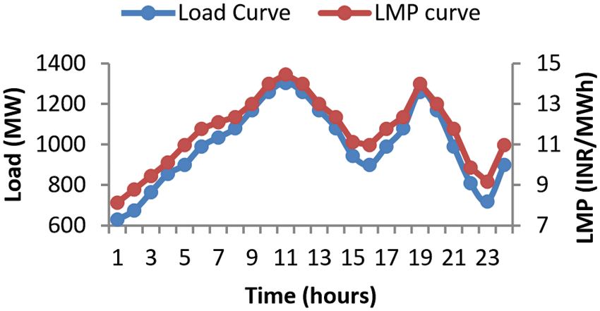
Figure 4: 24 h load curve and LMP curve
6.4 Implementation of DR Programs
Basic OPF problem incorporating different DRPs is implemented on IEEE 30 bus system. The 24-hour load demand is taken from Fig. 3. Depending on the demand, it is divided into three different periods, namely, valley period (00:00–5:00 h), off-peak period (5:00–9:00 h and 14:00–19:00 h), and peak period (9:00–14:00 h and 19:00–24:00 h). The initial spot electricity prices (i.e., ρo) are taken from the above LMP curve (Fig. 2) and the price elasticity of demand is taken from (Alami et al. 2010). The potential of implementing DRPs, i.e., “η” is considered to be 20%. The value of incentive, penalty, and spot electricity prices for each implemented DRPs are given in Tab. 1. For all DR programs, the OPF problem is solved by SFLA to determine the optimal dispatch by minimizing the operating cost. The number of populations is considered as 100 with 200 iterations. The algorithm is run for 100 trials and the best solution is presented. Economic allocation, voltage profile, and losses are also analyzed for each DR program.

6.5 Economic Analysis of Results
This case is solved with the actual load curve and without the implementation of any DR programs. The total load of the day is 23940 MW with a peak of 1305 MW. The average wind power is found by wind speed and power forecasting [27] and is taken as 80 MW. The total rating of energy storage capacities is assumed as 100 MW. The economic allocation without DR considering wind and energy storage and the total cost is INR 621378.
6.5.2 Program 1 (Direct Load Control)
In this case, DRP is modeled such that, as the electricity price increases above the average price of the day during peak hours, customers will tend to curtail their load. The spot electricity price is considered 11.6 INR/MWh (from the average LMP curve). The incentive INR 15 is given to the customers in peak hours for their load reduction. Compared to the base case, the system total load is now reduced by 7.3% (22161 MW) with a peak value reduction of 7.5% (1207 MW) and the total cost is INR 606889.
6.5.3 Program 2 (Capacity Market Program)
This is an incentive-based mandatory type of DRP, so the penalty is also included in this program. The value of incentive and penalty is considered as Tab. 1. Here the utility imposed interruption for peak hours 10, 11, and 12. In this case, the total incentive provided by the utility is INR 1028 for the load reduction of 3200 MW. Here the total cost of the system is reduced to INR 604744 with 13% of total power reduction compared to the base case.
6.5.4 Program 3 (Interruptible and Control Program)
This is an incentive and penalty-based market program. Penalty of INR 15 is imposed on the customer if they don't curtail the load as per the contract (i.e., 20% of the total load). Compared to the baseload, the total load reduction is around 17.5% (4207 MW) and the incentive and penalty costs are INR 1160 and INR 471 respectively. The optimal cost for this case is INR 609843. Further, the peak demand is also reduced by 18%.
6.5.5 Program 4 (Time of Use Program)
In this case, TOU rates are used with a very high price in critical peak periods i.e., INR 8, 10, and 13 at the valley, off-peak, and peak periods respectively. The demand reduction is achieved by about 1764 MW. Hence the total system cost is reduced to INR 597188, which is the lowest cost of all implemented DR cases.
6.5.6 Program 5 (Critical Peak Pricing)
In the CPP program with flat price rates (i.e., 11.6 INR/MWh), the price of INR 40 is considered for critical peak hours (10, 11and 12 h). In this case, the ED solution results in a total cost of INR 603378. Compare to the base case, during critical peak hour load profile is improved and peak reduction of 10.5% is achieved. Total power consumption is also reduced to 22824 MW. (vii) Program 6 (Real Time Pricing)
RTP is the time-based DRP in which no incentive or penalty will be imposed. The price structure considered for RTP is taken from ACOPF. In this case, the total demand for the system is reduced to 22101.
MW, with a system peak of 1267 MW. Here, an energy reduction of 7.68% is attained concerning the base case.
Results from these DRPs have been tabulated in Tabs. 2 and 3. Economic analysis of results shows the cost comparisons of each implemented DRPs. Power consumption comparisons exhibit changes in energy consumption with peak demand reductions for each implemented DRPs. Fig. 4 displays the impact of each implemented DRPs on the load profile of the system. As shown in Fig. 5, the highest peak reduction is achieved with the I/C program. Maximum reduction in energy consumption is achieved in the I/C program followed by CAP and RTP.
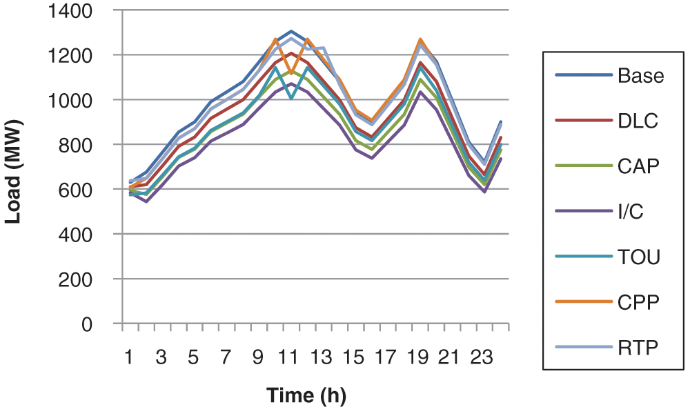
Figure 5: Load curve for different demand response programs


6.6 Analysis of Voltage Profile and Losses in DRPs
The simulation results and the influence of considered DRPs on voltage profile and losses are discussed in this section. On application of different DRPs, the variations in load demand bring changes in the voltages at each bus and also the losses associated with it. The volunteered buses for load curtailment are buses 8, 9, 10, 21, 22, 24, 28, and 29. The uniform load curtailment at all volunteered buses (max of 20% of load) is carried out for all DR programs. From the results, it is seen that with load curtailment, voltage profile is improved with the decrease in the losses. The voltage deviations and losses for each DRP are presented in Tab. 4. I/C DR program ranks first among the different DR programs. Hence, considering this DR program, OPF is run for this reduced demand and compared with the base case for the 11th hour (Peak hour) and the results are presented in Tab. 5. With the I/C program, 20% of the load is curtailed at that hour.


Under the deregulated market different demand response programs have been considered. Demand response is one of the emerging fields in the deregulated market to achieve better load regulation and for the reduction of cost. The economic analysis of different DRPs has been carried out for IEEE 30 bus system. This study shows that the customer's demand is largely influenced by the price elasticity, electricity price, and the incentive and penalty values determined for the concerned DRPs. Results show the reductions in demand of customers under different DRPs. I/C program gives the best result among all DRPs. Incorporating SFLA to solve OPF gives the optimum scheduling to reduce the total cost of the system. Further voltage deviations and losses are also being reduced by the DRP implementation. It is confirmed that by implementing DRPs, a reduction in total cost can be achieved with an enhanced voltage profile.
Acknowledgement: We thank our management, beloved Principal, and our Head of the department.
Funding Statement: The authors received no specific funding for this study.
Conflicts of Interest: The authors declare that they have no conflicts of interest to report regarding the present study.
1. M. I. Mosaad, A. Abu-Siada, M. M. Ismaiel, H. Albalawi and A. Fahmy, “Wind enhancing the fault ride-through capability of a DFIG-WECS using a high-temperature superconducting coil,” Energies, vol. 14, no. 19, pp. 6319, 2021. [Google Scholar]
2. A. A. E. Tawfiq, M. O. A. El-Raouf, M. I. Mosaad, A. F. A. Gawad and M. A. E. Farahat, “Optimal reliability study of grid-connected pv systems using evolutionary computing techniques,” IEEE Access, vol. 9, pp. 42125–42139, 2021. [Google Scholar]
3. A. Alhejji and M. I. Mosaad, “Performance enhancement of grid-connected PV systems using adaptive reference PI controller,” Ain Shams Engineering Journal, vol. 12, no. 1, pp. 541–554, 2021. [Google Scholar]
4. Y. Li, Z. Zhang, Y. Yang, Y. Li, H. Chen et al., “Coordinated control of wind farm and VSC–HVDC system using capacitor energy and kinetic energy to improve inertia level of power systems,” International Journal of Electrical Power and Energy Systems,” vol. 59, pp. 72–92, 2014. [Google Scholar]
5. W. Jia, C. Kang, D. Li, Z. Chen and J. Liu, “Evaluation on capability of wind power accommodation based on its day-ahead forecasting,” Power System Technology, vol. 36, pp. 69–75, 2012. [Google Scholar]
6. M. Ulagammai and R. P. K. Devi, “Wavelet neural network based wind speed forecasting and wind power incorporated economic dispatch with losses,” International Journal of Wind Engineering, vol. 39, no. 3, pp. 237–252, 2015. [Google Scholar]
7. S. Dhivya, M. Ulagammai and R. P. K. Devi, “Performance evaluation of different ANN models for medium term wind speed forecasting,” International Journal of Wind Engineering, vol. 35, no. 4, pp. 433–444, 2011. [Google Scholar]
8. H. A. Aalami, M. P. Moghaddam and G. R. Yousefi, “Demand response modeling considering interruptible/curtailable loads and capacity market programs,” Applied Energy, vol. 87, pp. 243–250, 2010. [Google Scholar]
9. A. Abdollahi, M. P. Moghaddam, M. Kazem and M. K Sheikh-EL-Eslami, “Investigation of economic and environmental-driven demand response measures incorporating UC,” IEEE Trans on Smart Grid, vol. 3, no. 1, pp. 12–25, 2012. [Google Scholar]
10. W. Junli, Z. Buhan, L. Hang, Z. Li, Y. Chen et al., “Statistical distribution for wind power forecast error and its application to determine optimal size of energy storage system,” International Journal of Electrical Power and Energy Systems, vol. 55, pp. 100–107, 2014. [Google Scholar]
11. D. Niu, S. Cao and J. Lu, Power Load Forecasting Technology and its Application, Beijing, China: Electric Power Press, pp. 1–8, 2009. [Google Scholar]
12. X. Chen, C. Kang and M. Chen, “Short term probabilistic forecasting of the magnitude and timing of extreme load,” Proceedings of the Chinese Society of Electrical and Electronics Engineers, vol. 31, pp. 64–72, 2011. [Google Scholar]
13. J. Hazra and A. K. Sinha, “A multi-objective optimal power flow using particle swarm optimization,” European Transactions on Electrical Power, vol. 21, no. 1, pp. 1028–1045, 2011. [Google Scholar]
14. B. Mahdad and K. Srairi, “A study on multi-objective optimal power flow under contingency using differential evolution,” Journal of Electrical Engineering and Technology, vol. 8, no. 1, pp. 53–63, 2013. [Google Scholar]
15. M. Samadi, M. H. Javidi and M. S. Ghazizadeh, “Modeling the effects of demand response on generation expansion planning in restructured power systems,” Journal of Zhejiang University Science, vol. 14, no. 12, pp. 966–976, 2013. [Google Scholar]
16. M. Marwan and F. Kamel, “Demand side response to mitigate electrical peak demand in eastern and southern Australia,” Energy Procedia, vol. 12, pp. 133–142, 2011. [Google Scholar]
17. Z. Tan, H. Li, L. Ju and Y. Song, “An optimization model for large–scale wind power grid connection considering demand response and energy storage systems,” Energies, vol. 7, pp. 7282–7304, 2014. [Google Scholar]
18. Q. Zhang, X. A. Wang and J. Wang, “Survey of demand response research in deregulated electricity markets,” Automation of Electric Power Systems, vol. 32, pp. 97–106, 2008. [Google Scholar]
19. W. Beibei, L. Xiaocong and L. Yang, “Day-ahead generation scheduling and operation simulation considering demand response in large-capacity wind power integrated systems,” Proceedings of the Chinese Society of Electrical and Electronics Engineers, vol. 33, pp. 35–44. 2013. [Google Scholar]
20. B. Wang and Y. Li, “Demand side management planning and implementation mechanism for smart grid,” Electric Power Automation Equipment, vol. 30, pp. 19–24, 2010. [Google Scholar]
21. O. Erdinc, “Economic impacts of small-scale own generating and storage facilities, and electric vehicles under different demand response strategies for smart households,” Applied Energy, vol. 126, pp. 142–150, 2014. [Google Scholar]
22. F. Pedro, S. Tiago, V. Zita and M. Hugo, “Distributed generation and demand response dispatch for a virtual power player energy and reserve provision,” Renewable Energy, vol. 66, pp. 686–695, 2014. [Google Scholar]
23. A. Manijeh, Z. Kazem and M. Behnam, “Short-term scheduling of combined heat and power generation units in the presence of demand response programs,” Energy, vol. 71, pp. 289–301, 2014. [Google Scholar]
24. H. Kuk-Hyun and K. Jong-Hwan, “Genetic quantum algorithm and its application to combinatorial optimization problem,” in Proc. of IEEE Int. Conf. on Evolutionary Computation, California, USA, IEEE, pp. 1354–1360, 2000. [Google Scholar]
25. K. Chandrasekaran, P. S. Sishaj and N. P. Padhy, “SCUC problem for solar/thermal power system addressing smart grid issues using FF algorithm,” International Journal of Electrical Power and Energy Systems, vol. 62, pp. 450–460, 2014. [Google Scholar]
26. A. Mohamed and M. Kowsalya, “A new power system reconfiguration scheme for power loss minimization and voltage profile enhancement using fireworks algorithm,” International Journal of Electrical Power and Energy Systems, vol. 62, pp. 312–322, 2014. [Google Scholar]
27. M. Ulagammai and R. P. K. Devi, “Wavelet neural network-based wind-power forecasting in economic dispatch: A differential evolution, bacterial foraging technology and primal dual-interior point approach,” Electric Power Components and Systems, vol. 43, no. 13, pp. 1–12, 2015. [Google Scholar]
 | This work is licensed under a Creative Commons Attribution 4.0 International License, which permits unrestricted use, distribution, and reproduction in any medium, provided the original work is properly cited. |