Intelligent Automation & Soft Computing DOI:10.32604/iasc.2023.026148
Article

Ensemble Based Learning with Accurate Motion Contrast Detection

M. Indirani* and S. Shankar

Hindusthan College of Engineering and Technology, Coimbatore, 641032, India
*Corresponding Author: M. Indirani. Email: mindirani2008@gmail.com
Received: 16 December 2021; Accepted: 27 February 2022

Abstract: Recent developments in computer vision applications have enabled detection of significant visual objects in video streams. Studies quoted in literature have detected objects from video streams using Spatiotemporal Particle Swarm Optimization (SPSOM) and Incremental Deep Convolution Neural Networks (IDCNN) for detecting multiple objects. However, the study considered optical flows resulting in assessing motion contrasts. Existing methods have issue with accuracy and error rates in motion contrast detection. Hence, the overall object detection performance is reduced significantly. Thus, consideration of object motions in videos efficiently is a critical issue to be solved. To overcome the above mentioned problems, this research work proposes a method involving ensemble approaches to and detect objects efficiently from video streams. This work uses a system modeled on swarm optimization and ensemble learning called Spatiotemporal Glowworm Swarm Optimization Model (SGSOM) for detecting multiple significant objects. A steady quality in motion contrasts is maintained in this work by using Chebyshev distance matrix. The proposed system achieves global optimization in its multiple object detection by exploiting spatial/temporal cues and local constraints. Its experimental results show that the proposed system scores 4.8% in Mean Absolute Error (MAE) while achieving 86% in accuracy, 81.5% in precision, 85% in recall and 81.6% in F-measure and thus proving its utility in detecting multiple objects.

Keywords: Multiple significant objects; ensemble based learning; modified pooling layer based convolutional neural network; spatiotemporal glowworm swarm optimization model

1  Introduction

Studies indicate recent surges in Significant Object Detections (SOD) [1] which is natural to humans who can easily identify visually distinctive areas in images. They identify based on dissimilar areas when compared with their surrounding regions [2–4] or they pay intrinsic attention to such differing image areas called SODs. Further, the rapid evolution of technologies has made it possible to trace significant image regions in digital images which has also paved the way for applications like object detection/recognition, compression of video frames/images, video tracing and healthcare image segmentations [5]. Studies have also demonstrated the possibility of object segmentations or SODs or motion tracings from videos [6,7]. Studies have also proposed solutions for discriminating significant objects in videos [8,9] by applying eye fixation tasks. Though they managed to distinguish objects as non-significant or significant, they failed to capture required features due to several factors.

Significant video regions were detection in [10]. The study presented a unified approach in constructing graphs for smoothing significant spatial-temporal regions for improving performances in large margins. A quick detection of significant video objects using Convolution Neural Networks (CNN) was presented in [11]. The study had two modules with one static and one dynamic model for capturing spatial and sequential scenes. The study in [12] projected a framework for enhancing model’s detection results by including spatiotemporal refinements, localized estimations and significant updates. The scheme was tested on 4 video dataset with good performances in terms of detections. The only drawback was in its obtained lesser precision.

KL divergence was used in [13] to detect video objects of significance efficiently. Scanty coding was used in the study to update pre attentive patch sets for identifying significant objects and for discriminations amongst them. Their scheme was found to be robust and achieved high precision value in experiments. Random Fields figured in the technique Spatio-Temporal Conditional Random Field (STCRF) proposed in [14]. The study found spatial relationships between video regions based on their temporal consistencies and proved its utility when tested on publicly available datasets.

Deep Neural Networks (DNNs) are being used in recent times to extract deep visual features of videos/images directly. These networks achieve these features from raw videos or images due to their higher discriminatory power and thus are modeled for systems detecting significant objects in videos. Most systems using DNNs established their supremacy over hand-crafted feature models in experimentations. One disadvantage found was in the accuracy of object detections while extracting deep features from independent frames on a frame by frame basis and specifically for dynamically moving objects.

Detecting Objects of Interest (OOI) in videos is more challenging than object detections in images. This is mainly because the motion blurs and ambiguities of moving objects. The complexity increases when objects are obstructed for a specific period of time while viewing them. Traditional object detection techniques use two frame detections where image frames have cluttered backgrounds. Hence, this study involves an ensemble approaches to detect multiple SODs efficiently from video streams.

The main aim of this research work is accurate motion contrast detection. There is numerous research and methodologies introduced but the analysis of performance is not ensured significantly. The existing approaches have drawback with accuracy and error rates. To overcome the abovementioned issues, in this research, Spatiotemporal Glowworm Swarm Optimization Model (SGSOM) is proposed to improve the overall detection performance. The main contribution of this research is detecting multiple significant objects. The proposed method is used to provide better results using effective approaches.

The rest of the paper is organized as follows: a brief review of some of the literature works in detecting multiple significant objects is presented in Section 2. The proposed methodology for accurate motion contrast detection is detailed in Section 3. The experimental results and performance analysis discussion is provided in Section 4. Finally, the conclusions are summed up in Section 5.

2  Related Work

The Significant objects were detected using visible background by the study in [15]. The study used Scale-Invariant Feature Transforms (SIFTS) for integrating long-range frames from multiple flow pairs. A bidirectional consistent obtained accurate temporal backgrounds. A bi-graph-based structure used these spatiotemporal backgrounds for computing significance of appearances and motions in information videos.

SODs in videos were also detected while detecting SODs near the border of frames, the detections may be incomplete. This study overcame this problem by joining virtual borders to detect SODs efficiently and accurately. The study in proposed Deeply Supervised Significant (DSS) object detections for improving SOD accuracy by introducing short connections in Holisitcally-nested Edge Detector (HED) architecture for skipping layer structures.

The study in detected SODs using a new method Spatiotemporal Constrained Optimization Model (SCOM). The work maximized energy functions for producing optimal significance maps for their processes. However, it performed better for single SOD. Spatiotemporal Particle Swarm Optimization Model (SPSOM) with IDL (Incremental Deep Learning) was proposed in for detecting multiple SODs. Incremental Deep Convolution Neural Network (IDCNN) subtracted foregrounds and backgrounds in images. Their proposed SPSOM identified globally optimized significant objects by constraining the object’s spatial/temporal data. Their scheme achieved higher and accurate detections.

High-accuracy Motion Detection (MD) scheme based on a look-up table (LUT) is proposed and experimentally demonstrated in an Optical Camera Communication (OCC) system. The LUT consists of predefined motions and strings that represent the predefined motions. The predefined motions include straight lines, polylines, circles, and number shapes. At the transmitter, the data with on-off keying (OOK) format is modulated on an 8 × 8 Light-Emitting Diode (LED) array. The motion is generated by the user’s finger in the free space link. At the receiver, the motion and data are captured by the mobile phone front camera. The captured motion is expressed as a string indicating directions of motion, then it is matched as a predefined motion in LUT by calculating the Levenshtein Distance (LD) and Modified Jaccard Coefficient (MJC). Using the proposed scheme, four types of motions are recognized accurately and data transmission is achieved simultaneously. Also, 1760 motion samples from 4 users are investigated over the free space transmission. The experimental results show that the accuracy of the proposed MD scheme can reach 98% at the distance without the loss of finger centroids.

Wang et al (2019) presented novel visual system model for small target motion detection, which is composed of four subsystems-ommatidia, motion pathway, contrast pathway, and mushroom body. Compared with the existing small target motion detection models, the additional contrast pathway extracts directional contrast from luminance signals to eliminate false positive background motion. The directional contrast and the extracted motion information by the motion pathway are integrated into the mushroom body for small target discrimination. Extensive experiments showed the significant and consistent improvements of the proposed visual system model over the existing models against fake features.

3  SGSOM Methodology

The proposed SGSOM system analyzes consecutive frame batches for detecting multiple SODs. In the SGSOM system foreground and background image subtractions are performed by an ensemble based learning which includes SVM (Support Vector Machine), MPCNN (Modified Pooling layer based CNN) and KNN (K-Nearest Neighbours). The proposed system is depicted as Fig. 1.

Figure 1: SGSOM framework for detecting multiple SODs

3.1 System’s Video Inputs

The proposed system aims to identify SODs in video frames depicted by Ft , t being the index of the frame. Assuming, regions with significant objects or backgrounds exist and analysis of spatial and temporal spaces in a video sequence help in the derivation of significant seeds in detected regions for achieving global optimization for SODs. The model segments regions using SLIC for generating super-pixels (Approximately 300 in number) in each video frame. Thus, SOD can be treated as a labeling problem of si (super-pixel) within a frame in the interval [0,1].

This work uses E(S), an energy constrained function for solving the super-pixel issue. If the set of super-pixels is denoted by R = { r1 , r2 , . . . , ri } in a spatial feature space S = { s1 , s2 , . . . , sN }, foregrounds are denoted by Φ, Γ depicts backgrounds and Ψ implies smoothness, then labels reliability can be found using Eq. (1)

E(S)=∑i=1N⁡Φ(si)+∑i=1N⁡Γ(si)+∑i,j∈N⁡Ψ(si,sj)+k (1)

where, k is the constraint vector of the energy minimizing function and N stands for spatially connected super-pixels pairs in the neighborhood within the frame Ft.

3.2 Ensemble Learning of the Proposed System

Ensemble learning is used in the study to subtract foregrounds and backgrounds in images by involving SVM, MPCNN and KNN.

SVM: SVM separates multiple class instances by generating an optimal hyper-plane and maximizes its distance from class instances within a search space. This linear separation using margin maximization of SVMs is depicted in Fig. 2.

Figure 2: SVM linear separation using margin maximization

This optimal hyper-plane can be expressed as a function of Support Vectors (Nearest Instances). If the video dataset is depicted as D with n frames the function can be represented as Eq. (2):

D={(xi,yi)|xiϵRp{−1,1}withi=1,..,n} (2)

where yi -foreground/background classes corresponding to an entry point xi (input frames), p-number of feature vectors of x. Eq. (3) depicts SVM’s hyper-plane formation

w⋅x−b=0 (3)

which is a dot product of a normal vector (w) a vector x in the hyper-plane, for separating data linearly into two hyper-planes. A hyperplane in an n-dimensional Euclidean space is a flat, n − 1 dimensional subset of that space that divides the space into two disconnected parts. To define an optimal hyperplane it needs to maximize the width of the margin (w). If the data is linearly separable, there is a unique global minimum value. The region without data points between the planes is called the margin. Both Eqs. (4) and (5) define hyper-planes:

w⋅x−b=1 (4)

w⋅x−b=−1 (5)

with 2/||w||-distance between hyper-planes. A constraint defined in Eq. (6) avoids data points in the margin.

yi(w⋅xi−b)≥1i=1,…,n (6)

Thus, a strong margin is formed when ½ ||w||2 gets reduced to the described constraint. Classifications may have errors and can be avoided by modifying the constraint as depicted in Eq. (7)

yi(w⋅xi−b)≥1−ξi,i=1,..nandξi≥0 (7)

The resulting OF (Objective Function) is expressed in Eq. (8)

OF=w,ξ,bmin{12||w||2+C∑i=1n⁡ξi} (8)

MPCNN: This work uses MPCNN to subtract foregrounds and backgrounds in frames. CNNs are generally tri-layered and operate with convolutional, sub-sampling and fully connected layers Video frames are the input and output layer with intermediate hidden layers and is depicted in Fig. 3.

Figure 3: MPCNN

This work’s MPCNN uses 8 layers with 3 sub-sampling layers, 3 CNN layers and 2 fully connected layers. CNNs enclose local pooling for improving computational efficiency and robustness when inputs vary. Local/average/max pooling methods fail to minimize loss of information. This work uses a convex weight based pooling layer to overcome this issue. Video frames form the input for convolution layer which has 16 kernels of 5 × 5 size. Each input is independently convolved with the kernel for n output frames. CNN’s first two layers is of size 5×5 while the last layer is 1×1 and n filters in each convolution layer are convolved with input for generating maps n∗ (specific frames) which is equal to the filters applied in convolution operations.

The lth output of the convolution layer denoted as Cj(l) is made of maps computed using Eq. (9)

Ci(l)=Bi(l)+∑j=1ai(l−1)⁡Ki,j(l−1)∗Cj(l) (9)

where, Bi(l) - Bias matrix, Ki,j(l−1) -convolution filter which connects jth feature with the ith frame on a one-to-one basis within the same layer. Ci(l) -output layer consists with feature maps, Ci(l−1) -1st convolution layer in the input space or Ci(0)=Xi ; The activation function applied as a non-linear transformation of the outputs of the convolution layer on the kernel generated frame map can be expressed as Eq. (10)

Yi(l)=Y(Ci(l)) (10)

where, Yi(l) -activation function output and Ci(l) -input. The activation functions used are sigmoid functions, tan h, and ReLUs (Rectified Linear Units) denoted as Yi(l)=max(0,Yi(l)) . These functions are used in deep learning models for reducing non-linear effects and interactions. The ReLUs convert outputs to 0 on negative inputs, while returning same input value when positive. These activation functions train faster due to error derivatives which are minimized in the saturating region and weight updates disappear also called the disappearing gradient problem.

Sub-Sampling: This layer comes after the convolution layer where this system’s CNN has 3 sub-sampling layers. Initial sub-sampling has a size of 2 × 2 while the last sub-sampling has 1 × 1 size. Sub-sampling reduces dimensionality of frame maps extracted from convolution layer. The outputs of convolution layer have 120 frame maps with 1×1 size. A part of global pooling layer is an important aspect in deep CNNs. A Convex weight based pooling layer in the proposed research work characterizes the pooling functionality. Local pooling operates on the cth channel map of an input tensor X ∈ RH × W × C can be depicted by Eq. (11)

Yqc=∑p∈Rq⁡wpcXpc (11)

where, {wpc}P∈Rq−convexweight and p, q-2-D positions on the input and output maps.

Fully Connected Layer: The proposed work used Softmax activation function depicted in Eq. (12) for outputs:

Yi(l)=f(zi(l)),wherezi(l)=∑i=1mi(l−1)⁡wHyi(l−1) (12)

where wH -weight value to be tuned by the fully connected layer for representing classes and f-transfer function representing non-linearity.

KNN: Video frames form the inputs for classification of backgrounds and foregrounds by KNN clustering as it classifies based on neighbor similarity. K value in this work is the frames used in classification. Euclidean Distances can be found using Eq. (13)

ED(x,y)=∑j=1k⁡(Xi−Yi)2 (13)

where, X-test samples and = (x1, x2, x3, · · · xn) and Y-database samples and = (y1, y2, y3, · · · yn)

For given inputs, the output probabilities from SVM, MPCNN and KNN is averaged before decisions. For an output i, the average output Si is given by Eq. (14):

Si=1n∑j=1n⁡rj(i) (14)

where rj (i)-output i of network j for input video frames. Different weights are applied for each network and validations have a lower error and larger weights when combining the results. Output probabilities from the combination of SVM, MPCNN and KNN are multiplied by a weight α before predictions and given in Eq. (15)

Si=∑j=1n⁡αjrj(i) (15)

This work computes a weighted mean for α value following Eq. (16)

αk=Ak∑i=1n⁡Ai (16)

where Ak–Validation accuracy for network k as i runs over n. The foreground and background are subtracted from images based on these average outputs.

3.2.1 Foreground Potential

In visually analyzing spatial features the foreground potential of significant object O’s regions can be computed from super-pixels ri in a frame Ft using Eq. (17)

Φ(si)=F(ri)(1−si)2 (17)

where F( ri )-Probability of super-pixel ri to be a foreground.

Motion energy term: This work uses motion energy M in its modeling where M encompasses a Significance map (St−1), distribution (Md), edge (Me) and history (Mh). Motion edges are generated using Sobel edge detectors which extract motion’s object contours in optical flows. A closer look at the spatial distribution of optical flows reveals that the background of objects in motion has a uniform color within frames and this distribution of motion can be depicted as Eq. (18)

Md(ri)=∑j=1N⁡||pt(rj)−μi||2vij (18)

where, ri -super-pixel, pt(rj) -super-pixel ‘s Normalized centroid and μi -super-pixel ‘s similar color weighted centroid. Previous studies on SODs extracted low-level features like texture from frames using center-surrounded maps (Mc). Initially, motion contrast M1 within frames is extracted in optical flows to model object motion clues. This contrast generated from the centre-surrounded map and distribution of motion is not inter-independent while locating objects in an optical flow. Their collective normalized motion contrast computations for each super pixel is done using Eq. (19)

M1(si)=Md(si)⋅exp(−γ⋅Mc(si)) (19)

where, γ -Balance factor, Md-Motion distribution, Mc -Center-surrounded map, si -Significant land space value . Hence, M1 represents the significance values derived from intra and inter frame information. It is difficult to maintain a steady quality in M1 due to inaccurate optical flows. The proposed system avoids inaccuracies from being uncorrected as even a single bad outcome of M1 can lead to propagation of errors. This work nullifies errors in contrast using consequent frame’s context information. Every contrast M1 map is split into grids for matching frames on a 1–1 basis using Eq. (20)

Dchebyshev(t,t′)=Lmax(||Ft(l)−Ft′)|| (20)

where, Dchebyshev(t,t′) -Chebyshev distance matrix, Ft(l) -Contrast Maps in time window (t = 1,2,···, M) with grids (L = 1,2,···, L), (t,t′) ∈ {1,2,···, M} (M = 5). The ratio of changes in contrast maps R(t) are computed by contrast comparisons with the lowest contrast within a batch ∑t′=1M⁡Dchebyshev(t,t′) and depicted as Eq. (21)

R(t)=∑t′=1M⁡Dchebyshev(t,t′)min(∑t′=1M⁡Dchebyshev(t,t′)) (21)

Thus, changes in maps found have their contrasts normalized based on using thresholds where Max R(t) > 1.3 results in repairing the map.

3.2.2 Background and Smoothness Potential

The background potential’s Γ(si) likelihood to be the background for each super-pixel for each super-pixel ri , as well is defined as Eq. (22)

Γ(si)=ωb(ri)si2 (22)

where ωb (ri) -background term for measuring probability of background for superpixel ri .

Smoothness potential paves the way for overall significance by assigning neighboring pixels with different significance labels and represented as Eq. (23)

Ψ(si,sj)=ωij(ri,rj)(si−sj)2 (23)

3.2.3 Reliable Object Regions

This work defines a reliable object region as O with B being its reliable background. Super-pixels within a region are clustered where cluster intensity I(ri) based on the pixel’s proximity to the cluster center is defined in Eq. (24)

I(ri)=∑ri,rj∈K⁡δ(||V(ri)−V(rj)||−dc) (24)

where dc is the proposed system’s non-sensitive cutoff value in the interval [0.05,0.5]. Delta function used in this work is depicted in Eq. (25)

δ(x)={1ifx<00otherwise (25)

The intensity values of a cluster imply super-pixels have greater number of neighbors within the cutoff distance and cluster centers have higher probabilities in being objects when they have lesser super-pixels in their neighbourhood when compared to the cluster intensity. Super-pixel of an object is selected when the intensity greater than threshold h0 and treated as a background super-pixel when intensity is lesser than threshold hb where these threshold values are obtained using Eqs. (26) and (27)

h0=t0∗max(I(ri)),ri∈K (26)

hb=tb∗min(I(ri)),ri∈K (27)

where, to and tb control cluster intensity’s spanning extent for O and B.

3.3 Multiple SODs

Relative significance of detected objects regions is used to predict SODs. This si done by defining an affinity matrix Woi∈RN×N from K super-pixels ro∈ O in all N ri∈ S and defined as Eq. (28)

Woi=[…,ωoi(ro,ri),..,ωKN(rK,TN) (28)

where,

ωoi(ro,ri)=exp⁡(−disc2(ro,ri)2σ2),(ro,ri)∈N (29)

Reliable background region for Wbi ∈ R RM×N is also defined from M super-pixels ∈ B to all ri ∈ S. SGSOM detects multiple significant objects and ranks them using GSO (Glowworm Swarm Optimization) which is inspired by lighting worm’s natural behaviour. Assuming these worms exist in random locations within a swarm, then each worm is a solution within a search space based on an objective function. The worms carry a certain amount of luciferin (positional fitness) where if they are bright implies that the solution is better. Worms with higher luciferin values attract other worms which have lesser brightness and their movement is towards the brighter ones. Thus, luciferin density determines local decisions within a domain or called its decision radius. Low densities result in extending their radius to attract more worms or split the swarm when intensity is very high. This merging and splitting is iterated till termination conditions are satisfied implying most worms gather around brighter glowworms. The main phases of the algorithm are initialization, luciferin-update, neighborhood selection, moving probability, movement and decision radius update phases. The proposed algorithm is depicted as Fig. 4. and its phases are detailed below.

Figure 4: Proposed algorithm for detecting multiple SODs

GSO initialization: Glowworms are super-pixels distributed randomly in fitness function space. The worms have equal luciferin quantities. Iteration is set to 1 and the distance between super-pixels is the fitness value in the proposed work.

Luciferin-updates: luciferin updates depend on fitness and prior luciferin values and guided by the rule given in Eq. (30)

li(t+1)=(1−ρ)li(t)+γFitnessxi(t+1) (30)

where, i-super pixel, li(t) -luciferin value of super-pixel at time step t, ρ -constant luciferin decay value where (0<ρ<1) , γ -constants for luciferin value enhancements, xi(t+1)εRM -super-pixel’s location at time step t and Fitnessxi(t+1) -super pixel fitness values at location in time step t+1 .

Neighborhood-Selection: Neighbors of super pixels i at t time Ni(t) have brighter ones written as Eq. (31)

Ni(t)={j:||dij(t)rdi(t)||;li(t)<lj(t) (31)

where i,j-super-pixels, rdi(t) -variable local-decision domain, di,j(t) -Euclidean distance between super-pixels at time step t.

The Euclidean distance between two points in Euclidean space is the length of a line segment between the two points. The collection of all squared distances between pairs of points from a finite set may be stored in a Euclidean distance matrix, and is used in this form in distance geometry.

Moving Probability: Super-pixels use a probability rule for getting closer to other super-pixels with higher luciferin values. The probability pij(t) of super-pixels (i, j) moving towards each other can be defined as Eq. (32)

pij(t)=lj(t)−li(t)∑k∈Ni(t)⁡lk(t)−li(t) (32)

Movements: When super-pixel i selects another super-pixel j ∈Ni(t) with pij(t) , the movement’s discrete-time model is given by Eq. (33)

xi(t+1)=xi(t)+s(t)(xj(t)−xi(t)||xj(t)−xi(t)||) (33)

where, S-step size, and ||.||-an Euclidean norm operator

Decision Radius Updates: The decision radius of a super-pixel is given by Eq. (34)

rdj(t+1)=min{rs,max{0,rdj(t)+β(nt−|Ni(t)|)}} (34)

where, β -constant, rs -sensory radius of super-pixel i, and nt -control parameter of number of neighbors.

4  Experimental Results

The proposed SGSOM was implemented in Matlab and benchmarked on the SegTrackV2 FBMS (Freiburg-Berkeley Motion Segmentation) and DAVIS (Densely Annotated Video Segmentation) datasets. SegTrackV2 items include girl, parachute, bird falls, cheetah, dog, monkey, penguin and many more items in short sequences of 100 frames, except for frogs and worms. The items taken for experimentations in this study are depicted in Fig. 5.

Figure 5: Snapshot of items taken for the study

Many video sequences were found to be motion-blurred in addition to objects with similar color backgrounds which made SODs a challenging task. The proposed system was experimented by splitting the datasets into training and testing sets where 29 video sequences from FBMS dataset was used in training and testing had 30 video sequences. Additionally, Davis dataset was used in experimentations as its 50 HD video sequences have dense annotations of frames.

4.1 Evaluation Metrics

5 standard metrics were used to measure performances including Precision, Recall, accuracy, f-measure and MAE (Mean Absolute Error) and the methods DSS (Deeply Supervised Significant) object detection, SCOM and SPSOM-IDCNN (Spatiotemporal Particle Swarm Optimization Model with Incremental Deep Convolution Neural Network) were taken for benchmarking SGSOM. Tabs. 1 and 2 represents the performance analysis of the proposed and existing approaches for SegTrackV2, FBMS and Davis datasets.

4.2 Performance Metrics of SGSOM

MAE: It is absolute errors average given by | ei| = | yi−xi| , where yi is the prediction and xi the true value. The mean absolute error is given by

MAE=∑i=1n⁡|yi−xi|n (35)

Fig. 6. displays this work’s proposed SGSOM’s comparative performance results with DSS, SCOM and SPSOM-IDCNN techniques on SegTrackV2, FBMS and Davis datasets in terms of MAE. Methods are denoted in the x-axis methods while their corresponding MAE values are plotted on the y-axis. This work’s ensemble-based learning performs well in SODs as it has reduced MAE values of 4.8% when compared to DSS, SCOM and SPSOM-IDCNN which have 22%, 15% and 9% respectively as their MAEs for SegTrackV2 dataset.

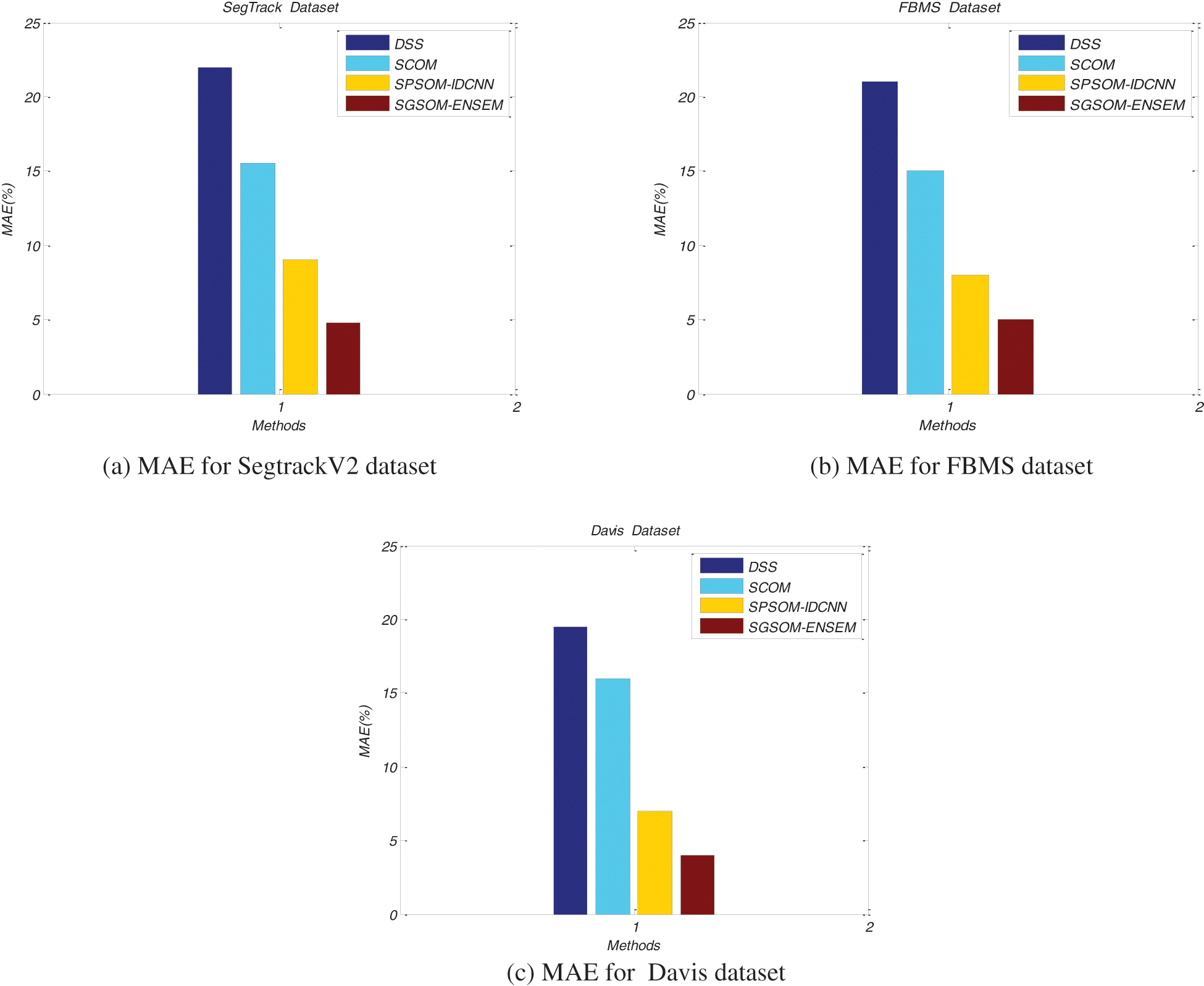
Figure 6: MAE comparison

Fig. 7 shows the accuracy of proposed SGSOM with ensemble approach and existing DSS, SCOM and SPSOM with IDCNN approaches for SegTrackV2, FBMS and Davis datasets. X-axis denotes methods while their accuracy values are plotted in the y-axis. From the graph, it can be concluded that SGSOM achieves 86% in accuracy while DSS, SCOM and SPSOM with IDCNN attains 73%, 77.5% and 81% respectively for SegTrackV2 dataset.

Figure 7: Accuracy comparisons

Fig. 8 shows the precision of proposed Spatiotemporal Glowworm Swarm Optimization Model (SGSOM) with ensemble learning approach and existing DSS, SCOM and SPSOM with IDCNN approaches for SegTrackV2, FBMS and Davis datasets. X-axis denotes methods while their precision values are plotted in the y-axis. The glow worm swarm is focused to generate best fitness values which are used increasing the motion detection accuracy. The proposed SGSOM achieves 81.5% in its precision whereas existing DSS, SCOM and SPSOM with IDCNN approaches attains 70%, 71.5% and 79% respectively for SegTrackV2 dataset.

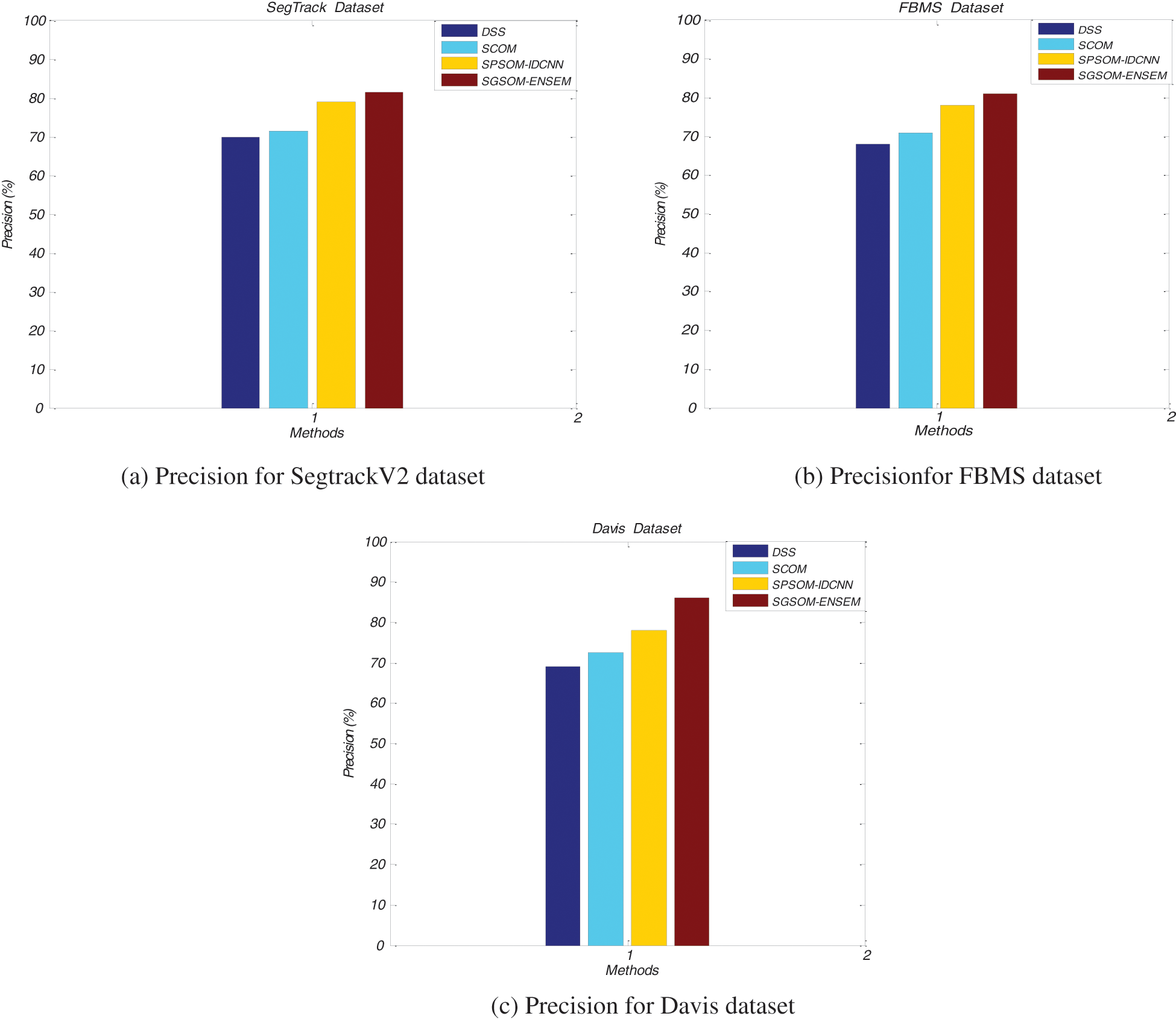
Figure 8: Precision comparisons

The recall of the proposed Spatiotemporal Glowworm Swarm Optimization (SGSOM) with ensemble learning approach and existing DSS, SCOM, SPSOM with IDCNN approaches are represented in Fig. 9. X-axis denotes methods while their recall values are plotted in the y-axis. The CNN extracts the important features from the given datasets and improves the detection accuracy higher. The proposed SGSOM achieves 85% in recall values when other methods such as DSS, SCOM, SPSOM with IDCNN achieves 71.2%, 75.3% and 78% respectively for SegTrackV2 dataset.

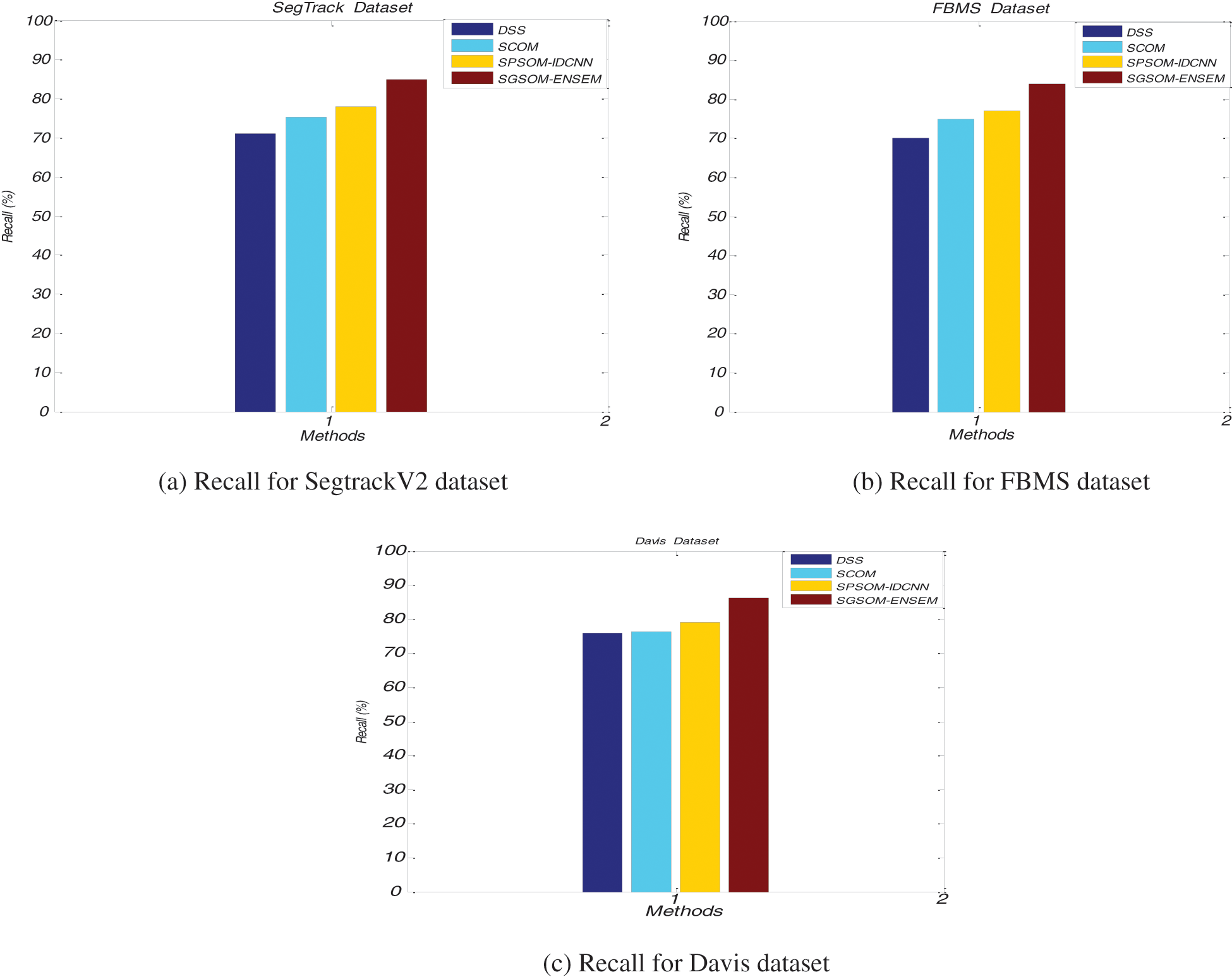
Figure 9: Recall comparisons

5  Conclusion

The proposed SGSOM detects multiple SODs from video sequences. Initially the foreground and background region subtraction is done using ensemble learning with SVM, MPCNN and KNN for attaining an optimal predictive model. Chebyshev distance matrix is computed to avoid inaccurate motion contrasts. This work’s SGSOM achieves a global significance optimization for multiple objects. It considers the distance between the super pixels as an objective function, thus enhancing its accuracy of SOD predictions. Thus, it is designed for global optimizations for detecting multiple SODs. SGSOM demonstrates its utility by scoring 86, 85 and 87 is accuracy percentage forSegtrackV2, FBMS and Davis datasets. It also outperforms other techniques used in experimental evaluations in terms of its higher precision, recall, f-measure and MAE values.

Funding Statement: The authors received no specific funding for this study.

Conflicts of Interest: The authors declare that they have no conflicts of interest to report regarding the present study.

References

 1.  X. Shen and Y. Wu, “A unified approach to Significant object detection via low rank matrix recovery,” in IEEE Conf. on Computer Vision and Pattern Recognition, Providence, RI, USA, pp. 853–860, 2012. [Google Scholar]

 2.  M. Iqbal, S. S. Naqvi, W. N. Browne, C. Hollitt and M. Zhang, “Learning feature fusion strategies for various image types to detect significant objects,” Pattern Recognition, vol. 60, no. 2, pp. 106–120, 2016. [Google Scholar]

 3.  G. Li and Y. Yu, “Deep contrast learning for significant object detection,” in IEEE Conf. on Computer Vision and Pattern Recognition, Las Vegas, NV, USA, pp. 478–487, 2016. [Google Scholar]

 4.  X. Li, L. Zhao, L. Wei, M. H. Yang, F. Wu et al., “Deep significance: Multi-task deep neural network model for significant object detection,” IEEE Transactions On Image Processing, vol. 25, no. 8, pp. 3919–3930, 2016. [Google Scholar]

 5.  L. Marchesotti, C. Cifarelli and G. Csurka, “A framework for visual significance detection with applications to image thumbnailing,” in 12th Int. Conf. on Computer Vision, Kyoto, Japan, pp. 2232–2239, 2009. [Google Scholar]

 6.  T. N. Le and A. Sugimoto, “Video significant object detection using spatiotemporal deep features,” IEEE Transactions on Image Processing, vol. 27, no. 10, pp. 5002–5015, 2018. [Google Scholar]

 7.  X. Zhou, Z. Liu, C. Gong and W. Liu, “Improving video significance detection via localized estimation and spatiotemporal refinement,” IEEE Transactions on Multimedia, vol. 20, no. 11, pp. 2993–3007, 2018. [Google Scholar]

 8.  S. Karthikeyan, T. Ngo, M. Eckstein and B. S. Manjunath, “Eye tracking assisted extraction of attentionally important objects from videos,” in IEEE Conf. on Computer Vision and Pattern Recognition, Boston, MA, USA, pp. 3241–3250, 2015. [Google Scholar]

 9.  W. Qiu, X. Gao and B. Han, “Eye fixation assisted video significance detection via total variation-based pairwise interaction,” IEEE Transactions on Image Processing, vol. 27, pp. 4724–4739, 2018. [Google Scholar]

10. K. Fu, I. Y. H. Gu, Y. Yun, C. Gong and J. Yang, “Graph construction for salient object detection in videos,” in 22nd Int. Conf. on Pattern Recognition, Stockholm, Sweden, pp. 2371–2376, 2014. [Google Scholar]

11. Z. Wang, J. Ren, D. Zhang, M. Sun and J. Jiang, “A deep-learning based feature hybrid framework for spatiotemporal saliency detection inside videos,” Neurocomputing, vol. 287, no. 2, pp. 68–83, 2018. [Google Scholar]

12. X. Zhou, Z. Liu, C. Gong and W. Liu, “Improving video saliency detection via localized estimation and spatiotemporal refinement,” IEEE Transactions on Multimedia, vol. 20, no. 11, pp. 2993–3007, 2018. [Google Scholar]

13. D. Y. Chen, C. Y. Lin, N. T. Yang and J. Y. Yu, “Sparse coding-based co-salient object detection with application to video abstraction,” in Int. Conf. on Machine Learning and Cybernetics, Tianjin, China3, pp. 1474–1479, 2013. [Google Scholar]

14. T. N. Le and A. Sugimoto, “Video salient object detection using spatiotemporal deep features,” IEEE Transactions on Image Processing, vol. 27, no. 10, pp. 5002–5015, 2018. [Google Scholar]

15. T. Xi, W. Zhao, H. Wang and W. Lin, “Significant object detection with spatiotemporal background priors for video,” IEEE Transactions on Image Processing, vol. 26, no. 7, pp. 3425–3436, 2016. [Google Scholar]

This work is licensed under a Creative Commons Attribution 4.0 International License, which permits unrestricted use, distribution, and reproduction in any medium, provided the original work is properly cited.