DOI:10.32604/iasc.2023.026424
| Intelligent Automation & Soft Computing DOI:10.32604/iasc.2023.026424 | |
| Article |
Optimized Neural Network-Based Micro Strip Patch Antenna Design for Radar Application
1Dhanalakshmi Srinivasan Engineering College, Perambalur, 621212, Tamil Nadu, India
2Sengunthar Engineering College, Tiruchengode, Namakkal, 637205, Tamil Nadu, India
*Corresponding Author: A. Yogeshwaran. Email: yogeshwaranaphd@gmail.com
Received: 25 December 2021; Accepted: 01 March 2022
Abstract: Microstrip antennas are low-profile antennas that are utilized in wireless communication systems. In recent years, communication engineers have been increasingly interested in it. Because of downsizing, novelty, and cost reduction, the number of wireless standards has expanded in recent years. Wideband technologies have evolved in addition to analog and digital services. Radars necessitate antenna subsystems that are low-profile and lightweight. Microstrip antennas have these qualities and are suited for radars as an alternative to the bulky and heavyweight reflector/slotted waveguide array antennas. A perforated corner single-line fed microstrip antenna is designed here. When compared to the basic square microstrip antenna, this antenna has better specifications. Because key issue is determining the best values for various antenna parameters when developing the patch antenna. Optimized Neural Network (ONN) is one potential technique utilized to solve this issue, and this work also uses Particle Swarm Optimization (PSO) to enhance the antenna performance. Return loss (S11) and Voltage Standing Wave Ratio (VSWR) parameters are considered in all situations, developed with Advanced Design System (ADS) applications. The transmitters are made to emit in the Ku-band, which covers a wide range of wavelengths. From 5–15 GHz, it is used in most current radars. The ADS suite is used to create the simulation design.
Keywords: Optimized neural network; particle swarm optimization; patch antenna; c-band; return losses
Wireless communication has been progressively evolving in recent years, including revolutionary antenna technology demands. The antenna structure is a critical component of many wireless communication systems, including wireless Local Area Network (WLAN), Wireless Fidelity (WIFI), mobile phones, traffic radar, Global Positing System (GPS), military, biomedical, and aerospace applications. Patch antennas arrays provide many advantages, including small dimensions, low density, low cost, high throughput, adaptability with horizontal or semi media, rapid manufacture, and connection of Minimum bactericidal concentration circuit. On top of a grounded dielectric material, a rectangle, square, triangle, or flat circular area is a basic microstrip patch shape Alamoudy et al. 2021 [1].
Apart from the well-known geometry, for multi-band operations, a compact leaves microstrip antenna patch is preferred. Other important features include a level head, lower exposure loss, and compatibility with microwave compact integrated circuits Bunea et al. 2020, Zbitou et al. 2006 [2,3]. In the electromagnetic spectrum, the X and Ku bands are independent and back-to-back. X/Ku bands are 8 to 12 GHz and 12 to 18 GHz, respectively, according to IEEE specifications. The Such Band is suited for a fast and secure satellite navigation system that supports central management stations and a large number of satellite earth interfaces. The Microstrip Bandpass interval supports voice, video and audio data transport, and video web conferencing services. The Very Small Aperture Terminal (VSAT) technology used on yachts and ships, on the other hand, is ideal for Ku Band applications. Antenna beams must be altered at Ku Band intervals to detect ship speed or displacement Alumona et al. 2014 [4].
Microstrip patch antenna design is analyzed via several approaches using Computer-Aided Design (CAD) software. Finite Elements Methods (FEM), MoM, and Finite Difference Time Domain (FDTD) are numerical computation methods with high computer system needs. The correlations between the design parameters of microstrips patch antennas and the patch dimensions are very nonlinear. Thus, the major purpose of employing an optimized neural network is to acquire a high degree of proper patch dimensions while using limited computing resources and neural networks. The following illustrative objects are motivated for this research work
i) The main objective is to design an antenna with the required properties to integrate different devices.
ii) This research compact design for microstrip antenna using slit and slot-loading in the ground plane of microstrip antenna has been studied. The technique to improve the bandwidth of microstrip antenna has also been studied.
iii) The design for operating a microstrip antenna at multiple resonant frequencies has also been studied.
iv) Finally, a design has been developed that may be used for its combined properties of compactness broadband and multiple resonant frequencies
This section discusses the literature survey based on traditional microstrip antenna procedures. Initially, met heuristic computations such as Genetic Algorithm (GA) and Particle Swarm Optimization (PSO) were used to optimize patch antennas. Later, Artificial Neural Network (ANN) was integrated, resulting in a hybrid soft computing approach Sarmah et al. 2020, Singhal et al. 2017, El-kenawy et al. 2021 [5–7]. In Chen et al. 2014 [8] GA was used to develop a microstrip patch antenna (which was simulated using HFSS) with a threefold increase in antenna bandwidth. In Dadgarnia et al. 2010 [9], a linear polarization microstrip patch antenna was developed (modeled using Simulation tool) and improved using a hybrid classification approach (trying to combine Classification model and Springfield), in which size parameters were predicted using a neural classifier and size variables were improved using Optimization method Dr. Rakesh Kumar et al. 2021 [10].
In Yudi Yuliyus et al. 2016 [11], the size characteristics of the dual stacking microstrip were reduced employing a hybrid soft computing technique merging Artificial neural and Swarm optimization Ramasamy et al. 2021 [12]. A hybrid classification strategy merging Evaluation metrics and Springfield is used to enhance the structural characteristics of a tux rectangular patch (represented using IE3D). Subsequently, Keerthi et al. 2021, Anand Kumar et al. 2020, Mohammad Saber Niazy et al. 2021 [13–15] used Discrete Particle swarm optimization to extend the size of an I-angled Z-shape rectangular microstrip directional antennas Z pattern (modeled using Simulation tool). Nawale et al. 2014 [16].
In particular, Pathak et al. 2021 [17] employs GA to improve the patches parameters of a novel-shaped microstrip line rectangular patch (designed to simulate with Measurements) that works in a variety of applications. In Kumar Singh et al. 2013 [18], a creative patch antennas antenna design (modeled with Periodic boundary conditions) with a Dipole Grooved Antenna (DGS) to improve specific capacity and a Differential Algorithm (DE) to maximize different specifications to reduce patch antenna calculation complexity, Beauchamp et al. 2021, Barros Cardoso da Silva et al. 2021 [19,20]. Based on this literature survey following problems are identified.
i) The microstrip antennas applications are limited because of portability, insufficient gain and higher cross-polar power levels concerning co-polar power levels.
ii) The narrow impedance bandwidth produces low gain; extra radiation from its feeds and connection points, handle low power, give less efficiency, and yield small polarization purity.
iii) The performance limitation of conventional microstrip antennas in low gain and low directivity values with small efficiency is also the major concern in its security application use
iv) The majority of the projects recommended are geared toward increasing bandwidth and decreasing size. Moreover, even though size small size is an important criterion in designing biological transmitters, this study focused on size micromachining as well as enhanced gain qualities of the suggested patch antenna by enhancing the size parameters (length, width) using PSO, making it suitable for biomedicine and ethnical applications.
The objective of the proposed wide-band microstrip is are to develop an accurate ONN-based synthesized model for CAD and other applications. The synthesized model can be used to calculate the human dimension of the wide-band microstrip for circular Defected Ground Structure (DGS) patch (a and r1) with required design frequency fmin and the parameter of a dielectric substrate (h, ɛr, ɛy and fr).
The Model’s input data of frequency response, density, and dielectrics of the insulating material are used to obtain the size of the microstrip antenna patches Fig. 1. The patch dimensions are calculated using the microstrip patch antenna’s specified formulae.
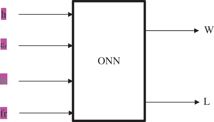
Figure 1: Patch antennas synthesis using ONN model
For such patch antenna estimation problem, the frequency response (fr) or both tops and bottom threshold levels are generated at the filter output of the ONN system, while the patched dimensions (W, L) and other variables (εr, εy, h) are supplied at the input side of the ONN model Fig. 2. These ONN models are easy to use and could aid researchers in determining exact top and bottom threshold frequency, throughput, frequency response, and patch antenna dimensions. The dielectric product’s electrical properties are indicated by εr and εy.
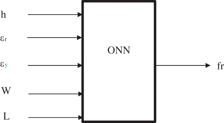
Figure 2: The analysis of microstrip patch using ONN technique
3.1 Optimized Neural Network (ONN) Architecture for Micro Strip Antenna
An ONN approach can be used to train a classifier in a range of methods. In this experiment, the neural network classifier and the ONN models for wearable antenna were built using a method of back-propagation. Connections are generated from either the nodes to the hidden and output layers in this manner. The system is designed using the conjugate gradient approach, with the estimated error being returned to the output neuron for, of course, further processing.
A deep neural network has two sets, one from the input to the output level and the other from the hidden units to the hidden layers. The delta method is being used to calculate the error generated by the second set of weights, and it must flow from the hidden layers to the input nodes for the error to be appropriately assigned to the lifts that produced it. The payout issue is used to identify which assessments should be updated and how frequently they should be changed.
The error back-propagation method, which has direct links, can be used to overcome this problem. It takes the input vector, calculates a function, and then assesses the derivative of the error function as follows of scores.
Backward pass: It computes the weight modifications by propagating the error derivatives backward.
This strategy employs the classification model. In multilayered feed-forward systems, there is normally one input source, one or a different number of unknown layers, and one output unit. The raw data is received by the input layer, the hidden layer performs the computations, and the activations are received by the output layer, which is then allocated to each pattern.
In this technique, smaller parts are used to examine how load influences the mistake, which is expressed by Eq. (1)
Because the direction of the mistakes, which might be positive or negative, can be established, partial derivatives are utilized. The back-propagation algorithm takes derivatives from the output layer’s weights to the input layer’s values.
A multiple fully connected feed-forward system is illustrated using the support vector method in Fig. 3. There are three levels in total: an input layer, a concealed layer, and an output layer. The input neurons are x1, x2, xn. The bias input is xb, and the related weight is w1b. Depending on whether w1b is positive or negative, the net output of the activation function might grow or decrease.
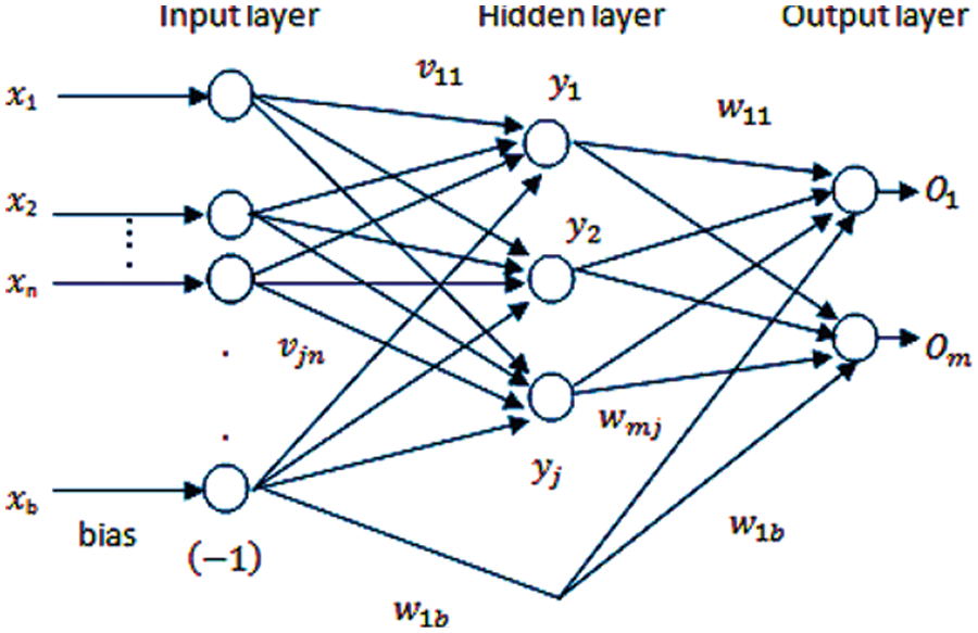
Figure 3: Optimized neural network
The output of w1b is kept consistent all through the method. It might be a 0 or a 1. y1, y2, yi are the hidden neurons, while O1, O2, Om are the outputs neurons. This means for input hidden state weights, represents the factor interconnected neurons to hidden layer neurons. Stands for outcome layer nodes and represents the factor given with hidden neurons connected to the output nodes. Vectors can be used to represent the input, hidden, and output layers, as shown in Eqs. (2)–(4).
where
t = the matrix’s transformation
P = learning pairings
x1, a1, x2, a2,…, xP, aP = there is askew
Output signal vectors reaction (a1, a2, and aP).
Step 1: To choose the Maximum Error for the condition η > 0
Step 2: E0, p 1, k 1, where E is the present error, p is the patterns counter, and k is the learning step response, are the masses set to a tiny random number.
Step 3: it’s time to start the training. The input layer receives the data, and the output is calculated using Eqs. (5)–(7).
Here f (.) = activation function
Step 4: Using Eq. (8), By integrating the previous minimum error, the objective function ak, and the overall outcome Ok, then can get the new error value.
Step 5: The error value for both layers is now calculated. The output layer’s error signal is computed using Eq. (9).
The bottom (invisible) gradient Amount of Errors is represented by Eq. (9).
Step 6: Eq. (10) is now used to alter the output layer’s weights:
3.1.2 Learning Factors of Optimized Neural Network
In this section discuss the operation of learning factors in optimized neural network. The starting weights, number of layers, number of neurons per layer, and updating strategy all influence the training of optimal neural networks.
Initial weight: The starting weights used to impact how quickly the networks converge. Initial weights are often chosen between −1.00 and 1.00 or −0.5 and 0.5. The starting weights of multilayer feed-forward networks may have an impact on the ultimate solution. The range
The system may not be adequately trained in all of the weights being set to the same value. If the weights are given large values just at the start, the network may become stranded at local minima very close to a start node. As a result, modest weights dispersed evenly across a narrow range must be employed to begin.
Learning rate (η): Back-propagation the learning rate has an impact on convergence. A large value merely speeds up closure, but it also introduces instability into the training algorithm, resulting in oscillations in the learned parameters; on the other extreme, a small value slows down learning. The range is between 10−3 and 10 for effective operation.
Several training data: The proportions or size of the input data to be categorized or customized with a given output quality determines the number of input layers. For training and testing, the training set should be adequate.
Momentum: When using small, the slope falls gradually, but when using large, it changes shape. The oscillation problem can be solved by adding a momentum component to the weight modifications as demonstrated.
where is the chosen velocity factor, with values ranging from 0.1 to 0.8. The momentum term is denoted by w (t-1). The present and most recent learning steps are indicated by the letters t and (t-1).
In the layers, several nodes are hidden: The size of the convolution layer in all layered feed-forward systems is established empirically. The layer must be a small percent of the input nodes for a system of suitable scale. If the system cannot resolve things, for example, further convolution layers may be required. When the system converges, however, the user will only be able to employ a few hidden layers.
Stopping criteria: When determining whether or not the network problem has been solved, halting criteria are employed.
i) When the mean squared error is sufficiently modest.
ii) The mean squared error rate of change is suitably low.
iii) A combination of the two requirements listed above.
Particle Swarm Optimization was employed as the optimization approach. Particle swarm optimization (PSO) is a reliable computing method based on the mobility and intelligence of swarms. The program’s PSO tool was used for the whole optimization procedure.
3.2 Optimization of Micro Strip Antenna Using Modified Particle Swarm Optimization
In this research, a new adaptive modal for such Optimization Algorithm is devised, wherein the cognitive component (C1) and even the learning element (C2) change with each cycle. The necessary parameters will be calculated (frequency range, dimensional width, defected ground height with plate thickness, electric depth, and dielectric loss vector). Our major goal is to test the efficiency of the new Particle Swarm Optimization technique for Org by changing the (C1, C2) amounts for each cycle (K).
The objective of this study is to use updated Particle swarm results to compute and evaluate the optimal particle error, physiological thickness, duty cycle, electrical width, micro strip radius (r), dissipation factor slope, and spectrum for circle radiating patch.
3.2.1 Modified PSO Algorithm for Circular Micro Strip Antenna (MSA)
As a result, PSO begins with particle locations and velocities that are picked at random. Each agent knows its optimal position, Pbest (the position vector in the optimization space), as well as the best location discovered by the entire swarm, Gbest. The Particle Swarm Optimization algorithm (PSO) works for the minimization problem of function f, i.e., optimizes the objective functions, by modeling the motion and interplay of the particle in a swarming. One of the problems is potential solutions or a point in the optimum space that correlates to the location of particles. Because we assume customers have no prior knowledge of the optimization problem, anyone can choose any point in the optimum space at any time during the optimizer. The velocity vector for the following iteration’s particle position computation is calculated as
where
Vn-1 = particle velocity in the previous iteration
w = inertia coefficient
r and ( ) = function that generates random numbers in the interval from 0.0 to 1.0
C1 = cognitive coefficient
C2 = social-rate coefficient.
The particle’s next location in the optimization space is computed as follows:
where Δt is the unit value, it is discovered that if there are no velocity limitations, particles may fly out of the specified optimization space. As a result, the maximum velocity Vmax is added to the PSO as a new parameter. Vmax is the greatest fraction of the optimizer variable’s range within which the photon’s mobility can fluctuate in consecutive passes.
Coefficients should be computed as soon as possible. For enhancing PSO obtained from regular PSO, consider the cognitive element and the social learning factor. The authors improved efficiency by modifying the cognitive factor (C1) and the social learning element (C2), demonstrating that the cognitive factor was necessary to seek the optimum place initially. After you’ve found the local best and have all of the information you need, you may look for the worldwide best. Coefficients should be computed as soon as possible. The Cognition Factor (C1) and the Social Learning Factor (C2) are used to improve PSO.
where
Ki = ith iteration
Kmin = predefined first iteration
Kmax =last or final iteration
Ki ≥ Kmax.
3.3 Performance Evaluation of Proposed Antenna
The following parameters validate the analysis of the method for radar applications
The impedance of Input: The value of Input Impedance of the suggested antenna design was calculated using the following mathematical Eq. (16).
where
XC1 = Capacitance output
XL1 = Inductance output
Analysis of stability: The factor is used to calculate LNA’s functional stability (K). The employment of the S-parameter is recognized, and the foreground equation is presented below.
where; |Δ| = |S11S22-S12S21| >1 with S11 < 1 and S22 < 1
The figure of Merit (FOM): The major variables that determine the Figure of Merit are power usage DC (Pdc), bandwidth (B), gain (G), intercepting point of final (IIP3), and fractional bandwidth (Wo). The following equation is used to compute the value of FOM (19).
Gain Analysis: The gain is calculated using the voltage ratio of the input (Vin) and output (Vout).
4 Experimental Setup and Results
Complementary Metal Oxide (CMOS) 90.18 m technology is used to create and measure the specified parameters using Advanced Design System (ADS) software. The preceding figures cover line ratio, gain, input reactance, backward isolation component, instability factor outputs radiation patterns, noise counts, voltage level, encompassing wave percentage range, energy consumption, and door voltage.
Fig. 4 depicts the suggested antenna design’s gain analysis. The proposed optimal neural network produced a maximum The S21 parameters value is14.65 based on the intended frequency response.
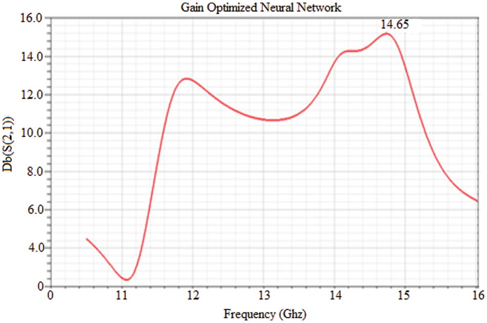
Figure 4: S21–optimized neural network
Fig. 5 shows a performance study of the Voltage Stranding Wave Ratio. The suggested Optimized Neural Network obtains a Voltage Standing Wave Ratio of 1.24 with a frequency of 9.68 based on the required frequency.
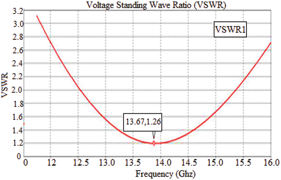
Figure 5: VSWR–optimized neural network
The simulation results of return loss (S11) by applying ADS software are shown in Fig. 6. The figure demonstrates that return loss is −11.2 dB at 15 GHz. Figs. 7 and 8 shows the Radiation Pattern in both 2D and 3D view.
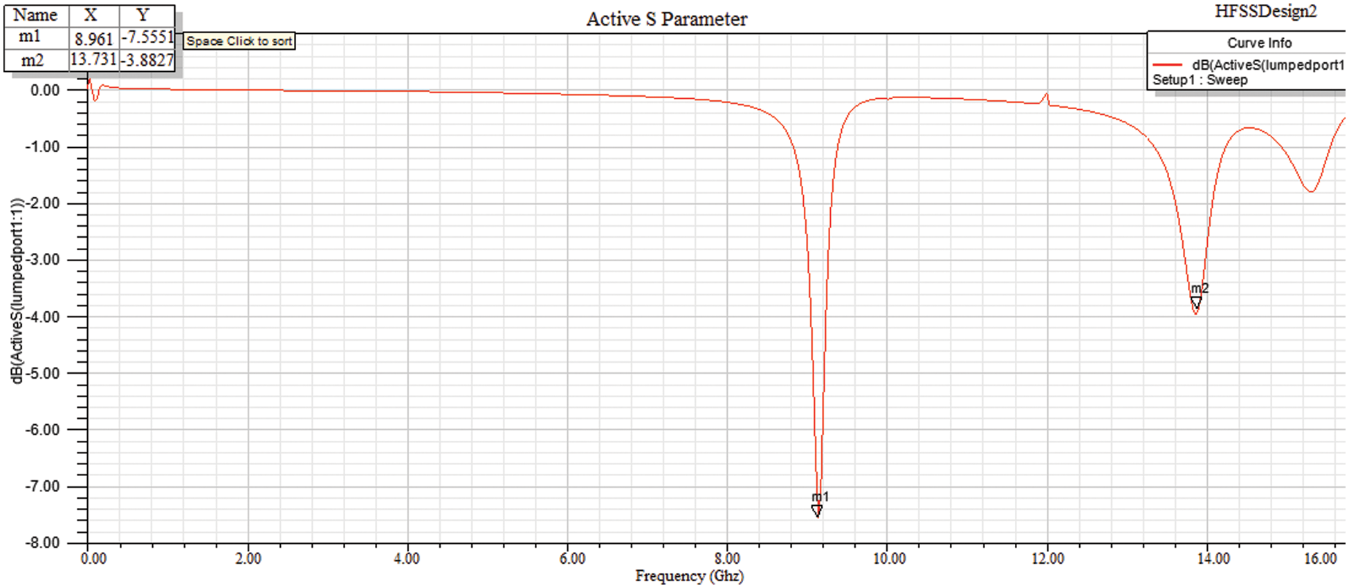
Figure 6: Simulation of the return loss vs. frequency of circular patch antenna
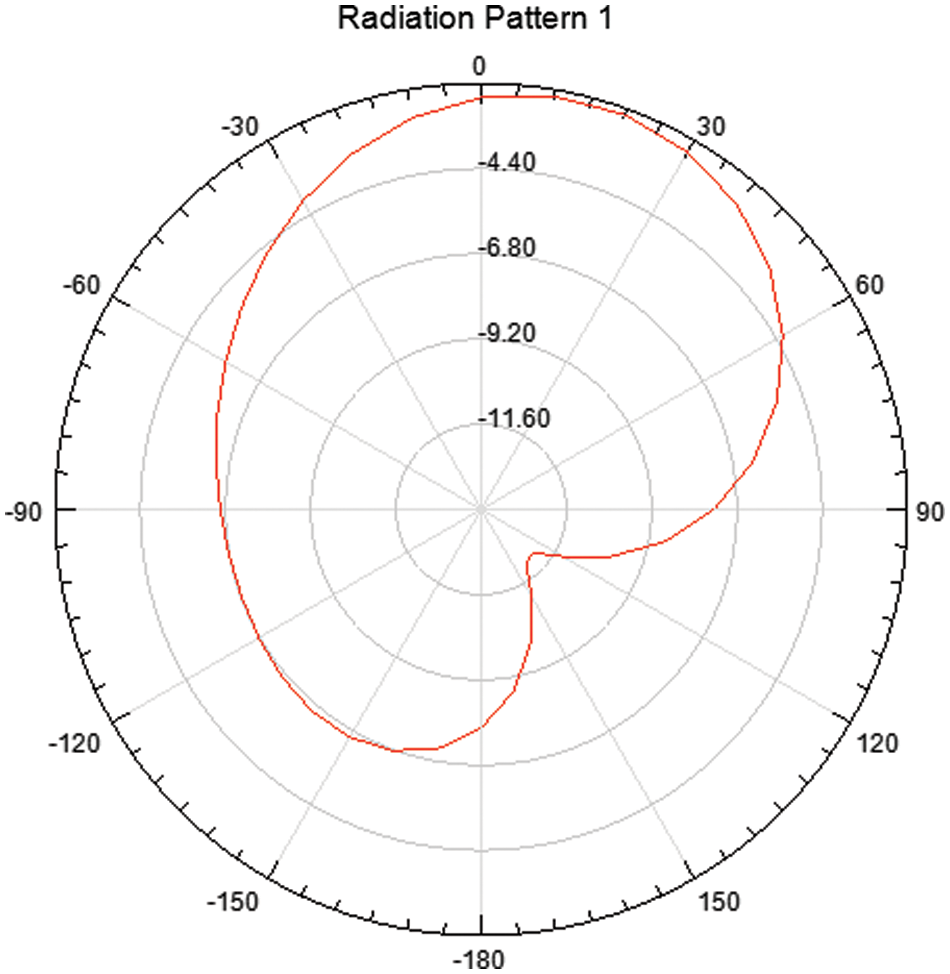
Figure 7: Radiation pattern
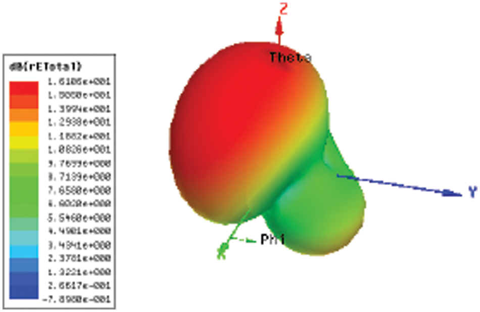
Figure 8: 3D view of radiation pattern
Tab. 1 shows the analysis study for several types of microstrip patch antenna designs. This table clearly shows that when compared to existing approaches, the suggested antenna design produces the best results. The noise Ratio of ONN, for example, is 0.265, the gain is 1.82, the Voltage Standing Wave Ratio is 1.24, and the Stability Factor is 1.81 (act1).
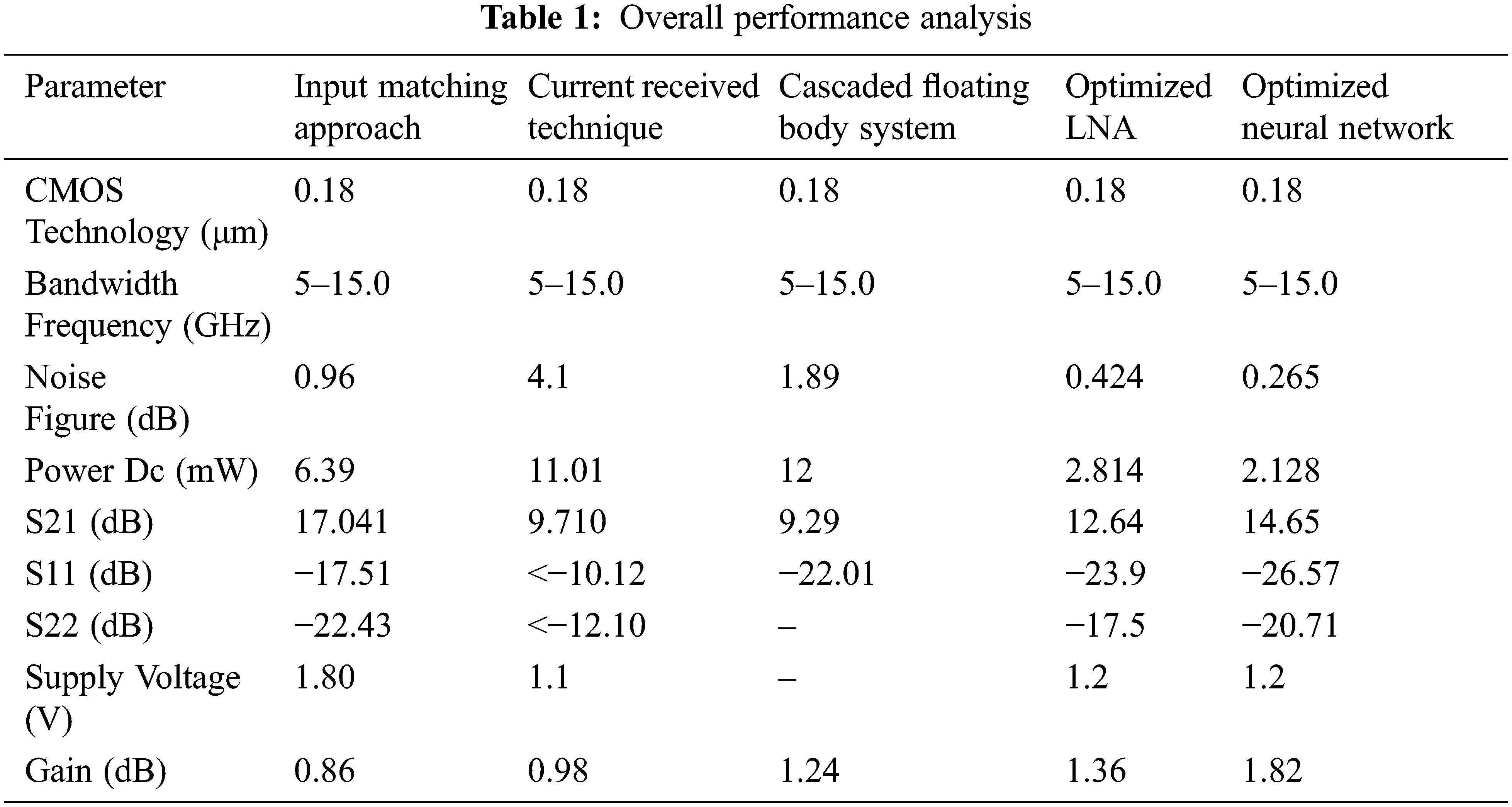
Using an improved neural network technique, a microstrip antenna arrangement for radar applications was constructed in this work. A simulation model was used to carry out the design and optimization process. The following statistics will include the waveform margin, yield, intake reactance, backward exclusion factor, instability factor outputs radiation patterns, noise counts, Input source, wave percentage range, energy consumption, and entrance voltage. To enhance the present System, the suggested microstrip antenna will be built utilizing the Fr4 substrate and studied using modeling and analysis such as radiation patterns, S-parameters, and return loss using ADS software. The suggested optimized neural network-based antenna performs well across the board, with noise ratios of 0.265, a gain of 1.82, a Voltage Standing Wave Ratio of 1.24, and a Stability Factor of 1.81 (act1). Micro strip patch antenna arrays will be studied in the future with various feed mechanisms for multiband applications.
Funding Statement: The authors received no specific funding for this study.
Conflicts of Interest: The authors declare that they have no conflicts of interest to report regarding the present study.
1. M. A. AL-Amoudi, “Study, design, and simulation for microstrip patch antenna,” International Journal of Applied Science and Engineering Review (IJASER), vol. 2, no. 2, pp. 1–29, 2021. [Google Scholar]
2. A. C. Bunea, D. Neculoiu, A. Stavrinidis, G. Stavrinidis, A. Kostopoulos et al., “Monolithic integrated antenna and schottky diode multiplier for free space millimeter-wave power generation,” IEEE Microwave and Wireless Components Letters, vol. 30, no. 1, pp. 74–77, 2020. [Google Scholar]
3. J. Zbitou, M. Latrach and S. Toutain, “Hybrid rectenna and monolithic integrated zero-bias microwave rectifier,” In Transactions on Microwave Theory and Techniques, vol. 54, no. 1, pp. 147–152, 2006. [Google Scholar]
4. T. L. Alumona, C. A. Ugbem and C. O. Ohaneme, “Overview of very small aperture terminal for television transmission,” American Journal of Engineering Research, vol. 3, no. 11, pp. 204–212, 2014. [Google Scholar]
5. K. Sarmah, G. Sivaranjan and S. Baruah, “Surrogate model assisted design of CSRR structure using genetic algorithm for micro strip antenna application,” Radio Engineering, vol. 29, no. 1, pp. 117–124, 2020. [Google Scholar]
6. M. Singhal and G. Sain, “Optimization of antenna parameters using artificial neural network: A review,” International Journal of Computer Trends and Technology, vol. 44, no. 2, pp. 64–73, 2017. [Google Scholar]
7. E. M. El-kenawy, H. F. Abutarboush, A. W. Mohamed and A. Ibrahim, “Advance artificial intelligence technique for designing double T-shaped monopole antenna,” CMC-Computers, Materials & Continua, vol. 69, no. 3, pp. 2983–2995, 2021. [Google Scholar]
8. G. Chen, H. Jiang and X. Lei, “Reconfigurable antenna design optimization based on improved quantum genetic algorithm,” XXXIth URSI General Assembly and Scientific Symposium (URSI GASS), IEEE, Beijing, China, pp. 1–4, 2014. [Google Scholar]
9. A. Dadgarnia and A. A. Heidari, “A fast systematic approach for micro strip antenna design and optimization using ANFIS and GA,” Journal of Electromagnetic Waves and Applications-J Electromagnet Wave Applicant, vol. 24, no. 16, pp. 2207–2221, 2010. [Google Scholar]
10. R. K. Joon and S. K. Vijay, “A review of various soft computing techniques in the domain of NANO-antenna design,” International Journal of Engineering Research & Technology, ICADEMS–2017, vol. 5, no. 3, pp. 1–4, 2017. [Google Scholar]
11. Y. Y. Maulana, Y. Wahyu, F. Oktafiani, Y. P. Saputra and A. Setiawan, “Rectangular patch antenna array for radar application,” TELKOMNIKA (Telecommunication Computing Electronics and Control), vol. 14, no. 4, pp. 1345–1350, 2016. [Google Scholar]
12. R. Ramasamy, V. Rajavel, C. N. Vasim Babuc, S. Vinoth Kumar and S. Parthiban, “Design and analysis of multiband bloom shaped patch antenna for IOT applications,” Turkish Journal of Computer and Mathematics Education, vol. 12, no. 3, pp. 4578–4585, 2021. [Google Scholar]
13. V. H. R. Keerthi, D. H. Khan and D. P. Srinivasulu, “Design of C-band micro strip patch antenna for radar applications using IE3D,” Journal of Electronics and Communication Engineering, vol. 5, no. 3, pp. 49–58, 2021. [Google Scholar]
14. D. Anand kumar and G. Sangeetha, “Design and analysis of aperture coupled micro strip patch antenna for radar applications,” International Journal of Intelligent Networks, vol. 1, pp. 141–147, 2020. [Google Scholar]
15. M. S. Niazy, F. Masood, B. Niazi, M. Rokhan and R. Ahmad, “Analysis of 3 × 4 micro strip patch antenna array for 94GHZ radar applications,” International Journal of Research in Engineering and Science, vol. 9, no. 9, pp. 43–50, 2021. [Google Scholar]
16. P. A. Nawale and R. G. Zope, “Design and improvement of micro strip patch antenna parameters using defected ground structure,” Journal of Engineering Research and Applications, vol. 4, no. 6, pp. 2248–9622, 2014. [Google Scholar]
17. S. Pathak and S. Kumar Singh, “Micro strip patch antenna: A review and the current state of the art,” International Research Journal of Engineering and Technology, vol. 8, no. 6, pp. 2395–0072, 2021. [Google Scholar]
18. K. Kumar Singh and D. S. C. Gupta, “Review and analysis of micro strip patch array antenna with different configurations,” International Journal of Scientific & Engineering Research, vol. 4, no. 2, pp. 6, 2013. [Google Scholar]
19. R. M. Beauchamp, S. Tanelli and O. O. Sy, “Observations and design considerations for space borne pulse compression weather radar,” in IEEE Transactions on Geoscience and Remote Sensing, vol. 59, no. 6, pp. 4535–4546, 2021. [Google Scholar]
20. A. B. C. da Silva, S. V. Baumgartner, F. Q. de Almeida and G. Krieger, “In-flight multichannel calibration for along-track interferometric airborne radar,” IEEE Transactions on Geoscience and Remote Sensing, vol. 59, no. 4, pp. 3104–3121, 2021. [Google Scholar]
 | This work is licensed under a Creative Commons Attribution 4.0 International License, which permits unrestricted use, distribution, and reproduction in any medium, provided the original work is properly cited. |