DOI:10.32604/iasc.2023.027442
| Intelligent Automation & Soft Computing DOI:10.32604/iasc.2023.027442 | |
| Article |
SMO Algorithm to Unravel CEED Problem using Wind and Solar
1Faculty of Electrical Engineering, Anna University, Chennai, 600025, India
2Department of Electrical and Electronics Engineering, AMET Deemed University, Chennai, 603112, India
3Department of Electrical and Electronics Engineering, Rajalakshmi Engineering College, Chennai, 602105, India
*Corresponding Author: A. Prabha. Email: prabhasresearch823@gmail.com
Received: 18 January 2022; Accepted: 20 February 2022
Abstract: This research proposes a more advanced way to address Combined Economic Emission Dispatch (CEED) concerns. Economic Load Dispatch (ELD) and Economic Emission Dispatch (EED) have been implemented to reduce generating unit fuel costs and emissions. When both economics and emission targets are taken into account, the dispatch of an aggregate cost-effective emission challenge emerges. This research affords a mathematical modeling-based analytical technique for solving economic, emission, and collaborative economic and emission dispatch problems with only one goal. This study takes into account both the fuel cost target and the environmental impact of emissions. This bi-intention CEED problem is converted to a solitary goal function using a price penalty factor technique. In this case, a metaheuristic and an environment-inspired, intelligent Spider Monkey Optimization technique (SMO) are used to address the CEED dilemma. By following the generator’s scheduling process, the SMO method is used to regulate the output from the power generation system in terms of pollution and fuel cost. The Fission-Fusion social (FFS) structure of spider monkeys promotes them to utilize a global optimization method known as SMO during foraging behaviour. The emphasis is mostly on lowering the cost of generation and pollution in order to improve the efficiency of the power system and handle dispatch problems with constraints. The economic dispatch has been remedied, and the improved result demonstrates that the system’s performance is stable and flexible in real time. Finally, the system’s output demonstrates that the system has improved in resolving CEED difficulties. When compared to earlier investigations, the proposed model’s findings have improved. As the generating units, wind and solar are used to explore the CEED crisis in the IEEE 30 bus system.
Keywords: Cost of generation; emission; CEED; thermal power system; bi-intention; SMO; wind and solar; IEEE 30 bus system
The economic dispatch (ED) problem has become a critical mission in terms of power system operational and strategic planning. Because the power supplier’s primary aim is to provide the finest economic strategy capable of convincing and fulfilling the demand for loads. Due to the consumption of fossil fuels during power generation, a thermal power station emits poisonous gases that pollute the environment. The thermal power station releases poisonous gases and damages the environment. Hence, it is important to minimize the use of these gases and the cost of fuel as much as possible for the welfare of society.
Over the last few decades, there have been numerous studies and techniques geared toward solving ELD issues. ELD problems are solved using techniques that have been around for a while, such as the gradient method, the lambda iteration method [1], linear programming, quadratic programming, the Lagrangian multiplier method, and the classical strategy based on co-ordination equations [2]. In addition to their computing complexity, these established methods will not work properly because they are sensitive to initial estimations and can be converged into optimal solutions.
Optimum power flow (OPF) provides the economic operation and balance of power and load flow situations were considered. While actual load flows for implementation and cost-effective power operation are examined in the OPF, social wellbeing is not given attention in this method [3]. The later Combined Economic Emission Dispatch (CEED) conveys more intent because it addresses the dual goal of emission and cost generation minimization [4]. CEED contains several local optimum solutions, and the algorithms developed are superior to conventional methods for arriving at the most effective global solution [5].
A substitute strategy is to make use of Evolutionary Algorithms (EA). EA is regarded as highly successful in dealing with the ELD problem since it can process non-linear objective functions. A Genetic Algorithm [6] (GA) is included in the EA technique [7] for optimization; the genetic algorithm is the most effective solution to the CEED, which focuses on environmental impact and cost generation. But convergence can take a very long time, depending on the size of the system. It also leads to the same, poor solutions being repeatedly reviewed.
The literature illustrates Simulated Annealing (SA) [8], yet this strategy can fail by being attracted to one of the optimal limited conditions. Evolutionary programming is addressed, and for large issues it has a sluggish convergence rate. An Enhanced Tabu search algorithm (TS) has been introduced [9], but the effectiveness of the algorithm has been compressed by using high target functions and optimizing several parameters. It’s also a long-term approach. The optimization of ant swarm (ASO) is provided, but its imaginary investigation is complicated and the allocation of probabilities changes with each iteration [10]. There was talk of Particle Swarm Optimization (PSO), but there is partial hope. In addition, the algorithm cannot solve the differentiation and optimization problems [11].
The cost efficiency transmit was resolved by means of differential evolution (DE) and has proven to be successful in finding the best answer globally [12]. The power system with the valve point loading has been well thought-out and DE was used for practical application. For solving static CEED, DE was utilized. CEED for IEEE test case6 was employed with GA and DE combinations [13]. The approach of colony bees [14] is employed to solve static CEED. The CEED is regarded as a dynamic CEED for one day, 24 h. For one day at a generating facility, it offers more realistic information. This dynamic CEED provides a world-class solution with real-coded GA. Non-linear generating features are considered in real load applications.
The Firefly algorithm (FA) replicates the clever technique of the firefly to solve engineering issues in the best way possible. A Flashing light based on an objective function is designed for optimization. This algorithm can be used to optimize or reduce difficulties. The Flower pollen algorithm (FPA) is a smart algorithm with an easy optimization procedure [15]. It imitates the process of reproducing flowering plants. The OPF is resolved by this FPA. In order to identify the best setup point, FPA offers a good worldwide solution [16].
SMO is a modern population-based flock intelligence method. When used to address universal optimization problems, it performs admirably. Hence, a new optimization strategy using spider monkeys was employed to resolve CEED problems. The functions and limits help to improve the system source. As a result, the system results are examined, and an optimum output is achieved with reduced processing time and costs.
Renewable energy systems with CEED problem mitigation have been studied in a number of reviews. Wind turbine generation is a function of wind speed. Different wind flows in this research are evaluated during the 24 h and this electricity is directly injected into the new generation power system. Solar power production is dependent on sunlight and is available throughout the day. Solar energy is estimated on the basis of the projected irradiation and directly introduced into the power system during its availability [17]. The multi-target feature is solved by employing the spider monkey optimization method [18–20] which has been successfully experienced in the IEEE 30-bus networks. The value of the spider monkey algorithm in solving CEED issues is proven with wind and solar energy penetration.
The CEED’s twin goals are to reduce generation fuel costs while also reducing emissions of poisonous gases such as sulphur oxides (SOx), carbon oxides (COx), and nitrogen oxides (NOx). To integrate these bi-intentions into one target, a price penalty factor is employed. For generation cost, quadratic cost equations are considered, and the VPL (valve point loading) effect is employed. The typical quadratic function of genuine power is observed and presented in the following equations for emissions.
where F is the total fuel cost in $/hr, F1 is the total cost of generation in $/hr, F2 is the total emission cost in ton/hr, h is the price penalty factor used to transform the bi intention into a single intention in $/ton, NG is the total number of generators used. The actual price performance coefficients are α, β, γ. The real power coefficients a, b, c, d and e are employed in the emission function.
To merge both objectives into one aim, the price penalty factor is applied. Emissions are assessed in ton/hr and converted into dollars/hr by increasing their price penalty factor. The final goal is therefore measured in dollars/hr. The price penalty factor of the ith generator is the highest quantity of production and the highest emission rate in the ith generation.
Subject to Inequality boundary conditions:
Equality load flow constraint:
where NT is the total number of transformers, NB–maximum number of buses allowed; MVAi–the i-th transmission line’s MVA flow; Vi–the voltage level of the i-th bus; Ti–i-th transformer’s tap position; PL and QL denote real and reactive power loss, respectively. The real and reactive power demand for load is denoted by PD and QD. Pgi, Qgi: real and reactive power generation of the generator.
α, β, γ are the fuel cost coefficients and ζ, λ are the valve point effect coefficients in the objective functions. The coefficients α, β, γ, ζ and λ are expressed in dollar/h, dollar/MWh, dollar/MW2 h, dollar/h and dollar/MWh, respectively. t/h, t/MWh, t/MW2 h, t/h and t/MWh are the respective units of emission coefficients a, b, c, d and e.
3 Spider Monkey Optimization Algorithm
The objective of swarm intelligence is to solve optimization disputes using a metaheuristic approach that is based on social species’ collective behavior. Social animals use their abilities to learn socially to tackle complex tasks. Earlier research has revealed that Swarm Intelligence algorithms have a strong potential to tackle the genuine difficulty in optimization. Over the last few years, the algorithms have included Particle Swarm Optimization (PSO), Bacterial Foraging Optimization (BFO), Firefly Algorithm (FA), Flower Pollination Algorithm (FPA), and so on.
3.1 Important Phases of SMO Algorithm
SMO is a population based algorithm with the following important phases. A Detailed description of SMOIA is delineated here.
3.1.1 Population Initialization
Initially, a population of N spider monkeys is represented by a D-dimensional series SMi where i = 1, 2,…, N and i symbolises the ith spider monkey. Each Spider Monkey (SM) symbolizes a possible outcome of the crisis under consideration. Each SMi is set up as follows:
In this case, SMminj and SMmaxj are the limits of SMi in the jth vector, and U (0, 1) is a random number in the range (0, 1).
3.1.2 Local Leader Phase (LLP)
The spider Monkey renews its present location in this phase, providing a fitness value based on the observations of the local leader and group mates. If the current location’s fitness measure is higher than the prior location’s, SM replaces it with the most recent one. As a result, the ith SM in the kth local group modifies its position.
Here, SMij defines ith SM in jth dimension, whereas LLkj shows a relationship to the kth leader of the local assembly location in jth dimension. SMrj characterizes rth SM which is indiscriminately picked from kth group such that r ≠ i in j th dimension.
3.1.3 Global Leader Phase (GLP)
The Global Leader (GLP) segment starts on following the completion of the Local Leader phase. In GLP, the entire SM updates its position using the awareness of the global leader, the skills of neighbouring SM, and its own individual determination. The location renewal equation is as follows for this phase:
Which GLj is a global leader’s jth dimension, and j ∈ {1, 2,…, D} is the random index chosen. The position of SMi is updated in this phase on the basis of a probability probi which is determined using its fitness. The superior candidate has more opportunities to improve itself. Probability probi can be evaluated using the equation
where fitnessi is the ith SM’s fitness value. In addition, it calculates and compares the suitability of the recently formed location of the SM with the old one and takes the better one.
3.1.4 Global Leader Learning (GLL) Phase
The location of the global leader is reorganized in this phase by using greedy choices in the population, i.e., the updated location of the global leader is the SM with the best fitness in the population. Furthermore, the location of the global leader is ensured to see if it is updated, and if it isn’t, the global limit count is increased by one.
3.1.5 Local Leader Learning (LLL) Phase
The location of the local leader is restructured in this phase by using greedy choices in that group, i.e., the updated location of the local leader is the SM with the finest fitness in that group. The local leader’s new location is then compared to the old one, and if the local leader has not been reorganized, the local limit count is increased by one.
3.1.6 Local Leader Decision (LLD) Phase
If the local leader location is not modified up to a pre-calculated limit known as the Local Leader Limit through an equation based on perturbation rate, the local leader location is updated in one of two ways: by random initialization or by blending information gained via global and local leaders (pr).
Evidently, the modified dimension of this SM is mesmerised by the global leader and opposes the local leader, as seen in Eq. (15). Furthermore, the modified SM’s fitness is evaluated.
3.1.7 Global Leader Decision (GLD) Phase
The location of the global leader is examined in this phase, and if no adjustment is made to the prearranged iteration limit, known as the Global Leader Limit, the population is separated into tiny crowds by the local leader. Initially, the population is divided into two classes, then three, four, and so on until the higher bounce, known as the group of greatest number (GN), is reached. In the intervening time, for freshly generated subclasses, local leaders are chosen using the LL approach. As a result, the suggested algorithm is modelled after the spider monkeys’ fission-fusion structure.
Fig. 1 shows the flowchart for the implemented SMO model. The parameter range requirements considered in the SMO algorithm are given below.
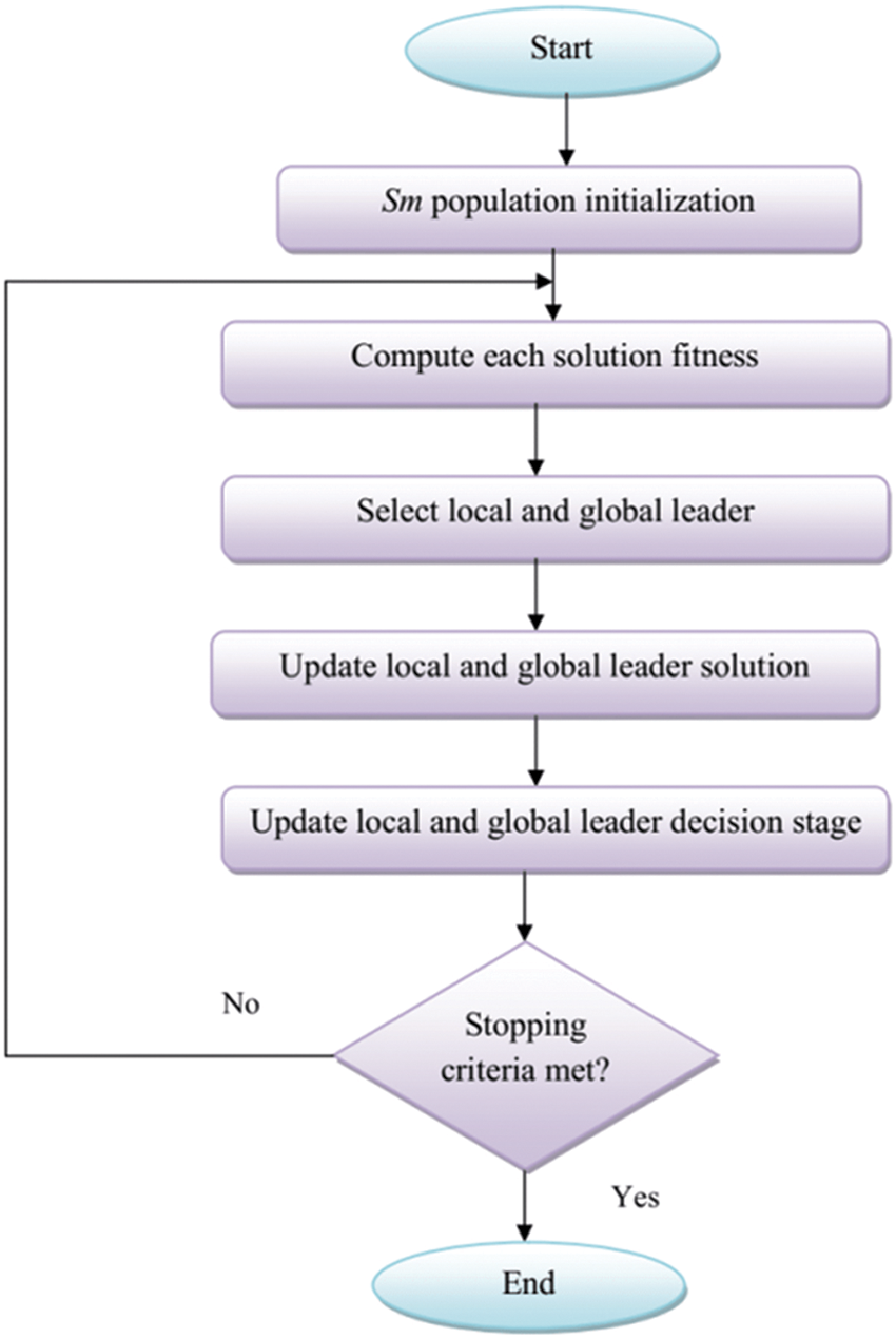
Figure 1: Implemented SMO model
3.2 Parameter Range Requirement Considered for SMO Algorithm
i) Maximum Group (MG)
ii) Local Leader Limit (LLL) must be D × N
iii) Global Leader Limit (GLL) must be ɛ [N/2, 2 × N]
iv) Perturbation rate (pr) ɛ [0.1, 0.8] where N is the group size.
4 Implementation of Developed Algorithm
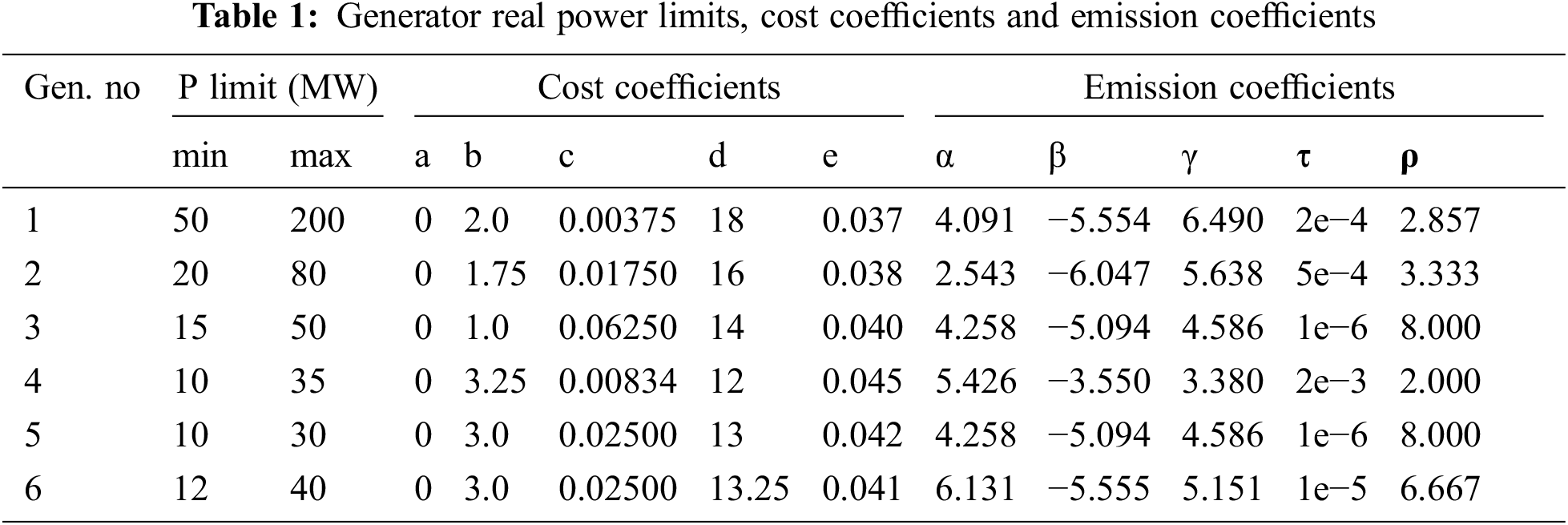
The SMO mathematical model is simulated using MATLAB. The typical IEEE 30 bus test case was utilized to optimize the spider monkey algorithm. It has 6 steam generators, 4 transformers and 41 transmission lines. The system base MVA is 100 MVA. There are 15 control variables: 4 for tap positions, 6 for bus voltages and 5 for real power generations. The challenge of CEED is to reduce the cost of fuel and emissions. Tab. 1 summarizes the cost-coefficient restrictions of the generator and the emission coefficients of the IEEE 30 bus system generator. The active and reactive power demand is 283.4 MW and 126.2 MVAR.
The six generator buses should have at least one slack bus for the reference location. The decision variables are the P and V of the generator buses, as well as the transformer tap locations. These decision variables must fall inside the boundaries of the test case. The generator’s dependent variable Q must be checked and kept within the limitations specified. The fuel cost for generating plants is calculated in $/hr using generation cost coefficients, while the emissions of generating plants are calculated in tonnes per hour using emission coefficients.
The results are addressed in terms of valve point loading and without valve point loading. The input-output characteristics of generating units are affected by valve point loading, making fuel prices nonlinear and unpredictable. This has been considered while addressing load dispatch challenges, but not when arranging unit committment. The info yield attributes are viable without valve point loading, bringing about a direct and steady fuel cost.
For the specified set of decision factors, the power flow of the power system with the standard NR load flow is calculated. This power flow re-estimates the decision variable. The population size of 20 spider monkeys, LLL, GLL, and pr is first assumed. The fitness of the spider monkey is computed based on an estimation of the individual spider monkey’s distance from food sources.
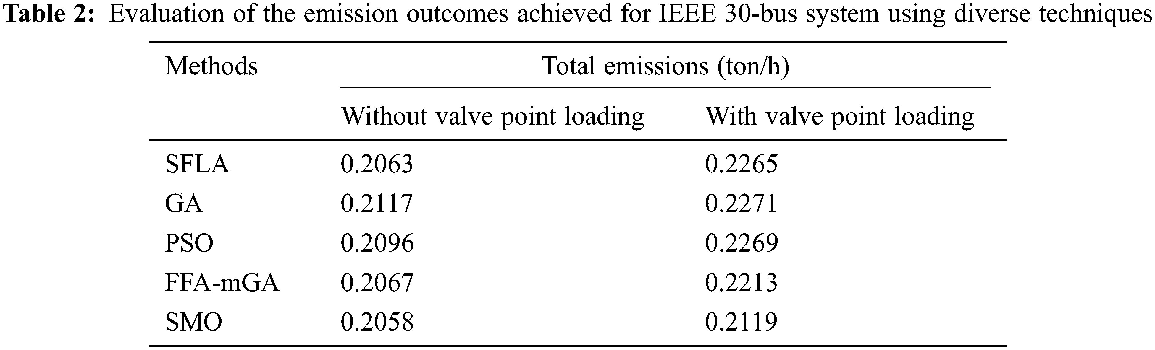
Tab. 2 depicts the emission minimization using the spider monkey optimization approach. It also assesses the outcomes of several emission reduction measures for the IEEE 30 bus technology. When no valve point loading is considered, the emission is 0.2058 ton/hr, and when valve point loading is considered, the emission is 0.2119 ton/hr. The convergence curves for emission reduction without and with valve point loading are shown in Figs. 2a and 2b.
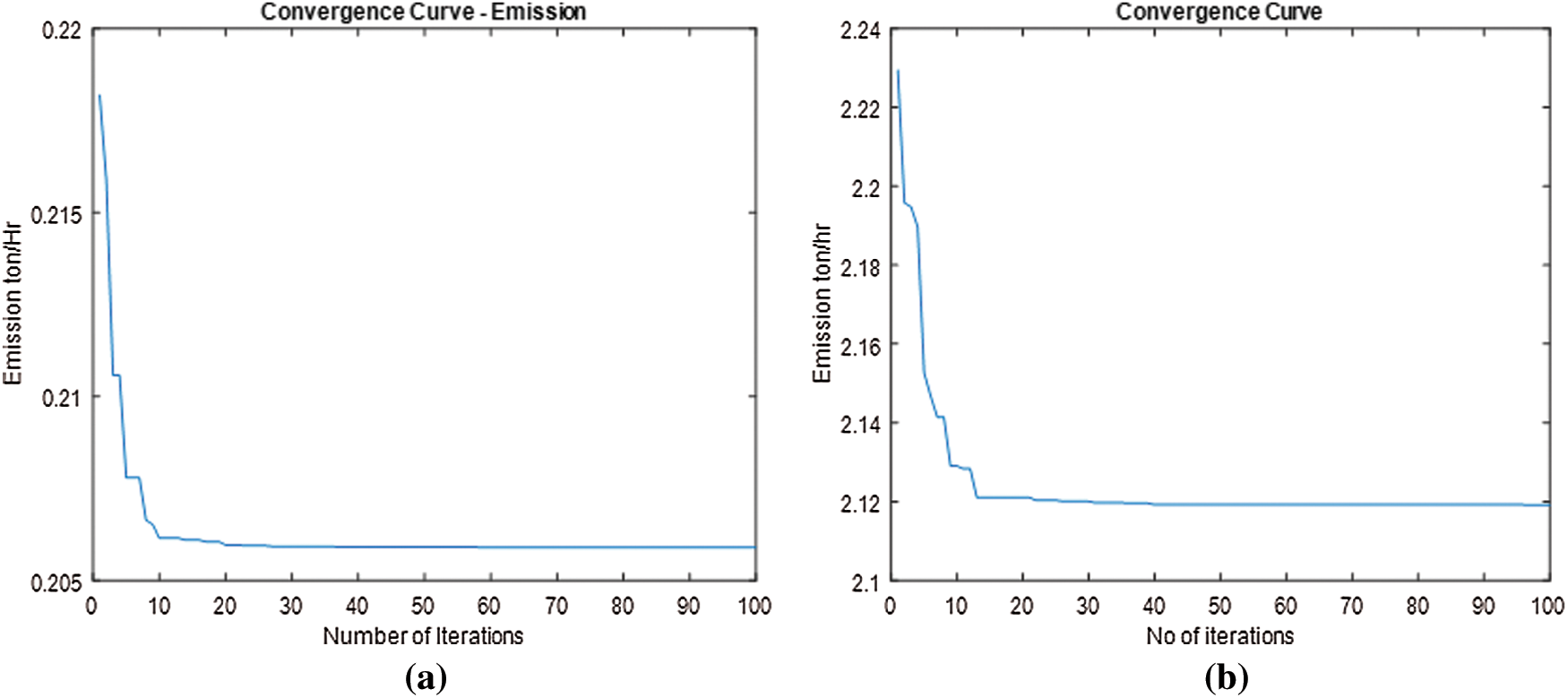
Figure 2: a) Convergence curve for emission reduction without valve point b) Convergence curve for emission reduction with valve point
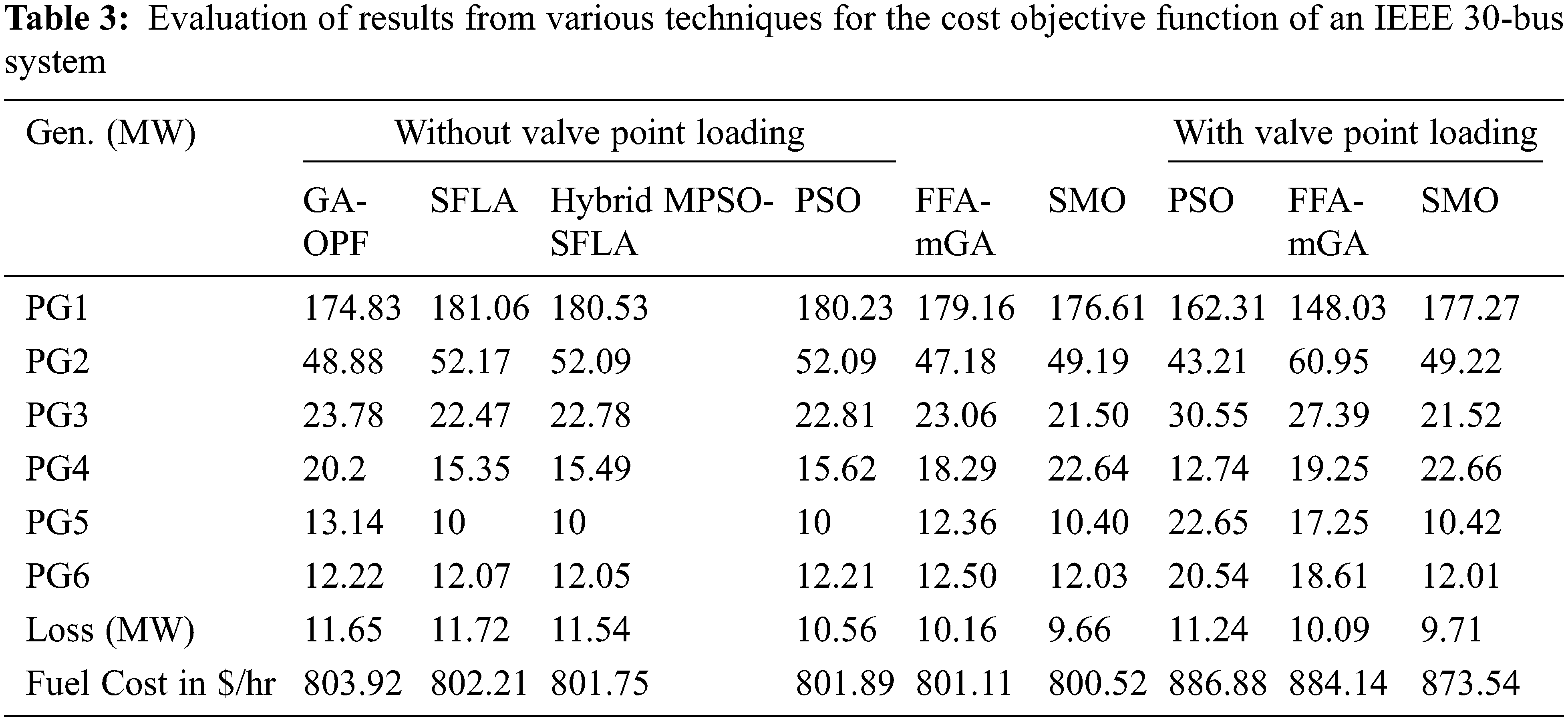
Tab. 3 illustrates the generating cost minimization using SMO and a comparison between SMO and various techniques for the cost objective function of an IEEE 30-bus network. By considering without valve point loading, the economic cost of minimization is 800.52 $/hr, while considering with valve point loading, the economic cost of minimization is 873.54 $/hr. Figs. 3a and 3b illustrate the convergence curve for generating a cost-minimization strategy without and with valve point loading.
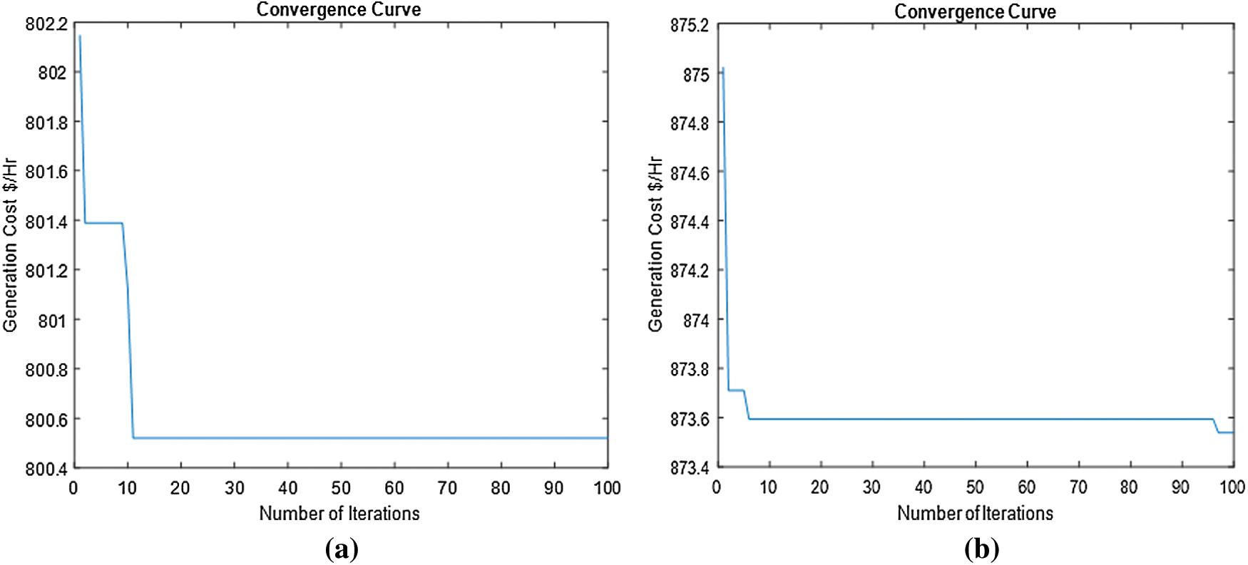
Figure 3: a) Convergence curve for generating cost minimization without valve point b) Convergence curve for generating cost minimization with valve point
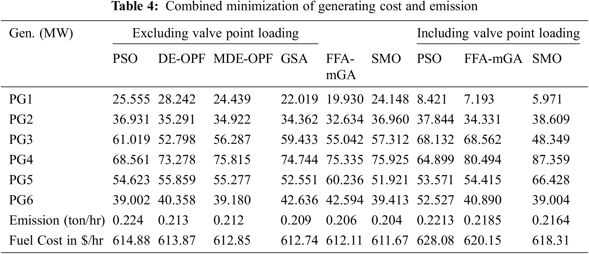
The combined minimization of generating cost and emission is shown in Tab. 4. This clearly shows that SMO provides the lowest generating cost and emissions when compared to PSO, DE-OPF, MDE-OPF, GSA, and FFA-mGA for the CEED issue. As compared to all other algorithms, the best possible fuel cost without valve point loading is 611.67 $/h at an emission of 0.204 tons/hr, and with valve point loading, the cost is 618.31 $/h at an emission of 0.2164 tons/hr. The convergence curves in Figs. 4a and 4b represent the CEED minimization, including and excluding valve point loading, with 100 iterations as the stopping criterion.
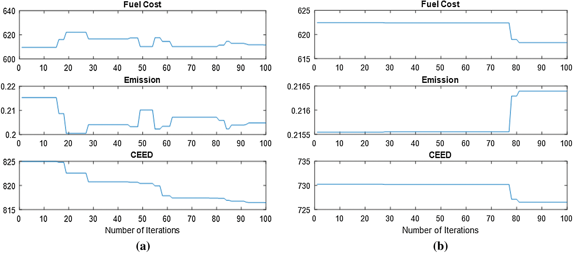
Figure 4: a) Convergence curve for the CEED Minimization without valve point b) Convergence curve for the CEED Minimization with valve point
The influence of wind and solar on CEED-SMO with and without VPL is shown in Tab. 5. Wind and solar power projections are supplied into the power grid as actual power and deducted from total genuine power demand. The committed generators are assigned to the net real power demand after removing renewable power. The allocation of the optimal producing pattern is optimized using SMO. The load requirement in a day is taken into account when implementing the designed algorithm.
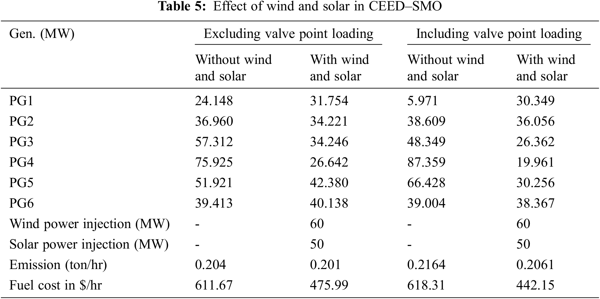
Fig. 5 shows the power generation in CEED with and without wind-solar power injection, excluding and incorporating VPL. When wind and solar power are injected, the power generation is enhanced in order to avoid valve point loading.
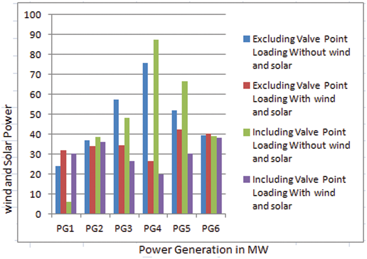
Figure 5: Power generation- with and without wind-solar power injection
Fig. 6 depicts the fuel cost in dollars per hour in CEED-SMO with and without valve point loading. In excluding valve point loading, the fuel cost is 611.67 $/hr, without wind and solar power. The fuel cost is 475.99 $/hr with wind and solar power. Including valve point loading, the fuel cost is 618.31 $/hr, without wind and solar power. The fuel cost is 442.15 $/hr with wind and solar power. As a result, without valve point loading, the input-output characteristics are effective, resulting in a linear and consistent fuel cost.
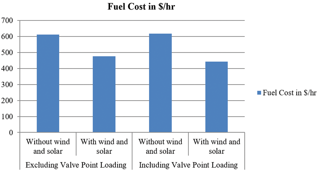
Figure 6: Fuel cost in $/hr in CEED-SMO
The emission in ton/hr in CEED-SMO is shown in Fig. 7, taking into account valve point loading and excluding the same. In excluding valve point loading, the emission is 0.204 ton/hr, without wind and solar power. The emission is 0.201 ton/hr with wind and solar power. Including valve point loading, the emission is 0.2164 ton/hr, without wind and solar power. The emission is 0.2061 ton/hr with wind and solar power. As a result, even when no valve points are loaded, the input-output properties are valuable, resulting in linear and constant emission.
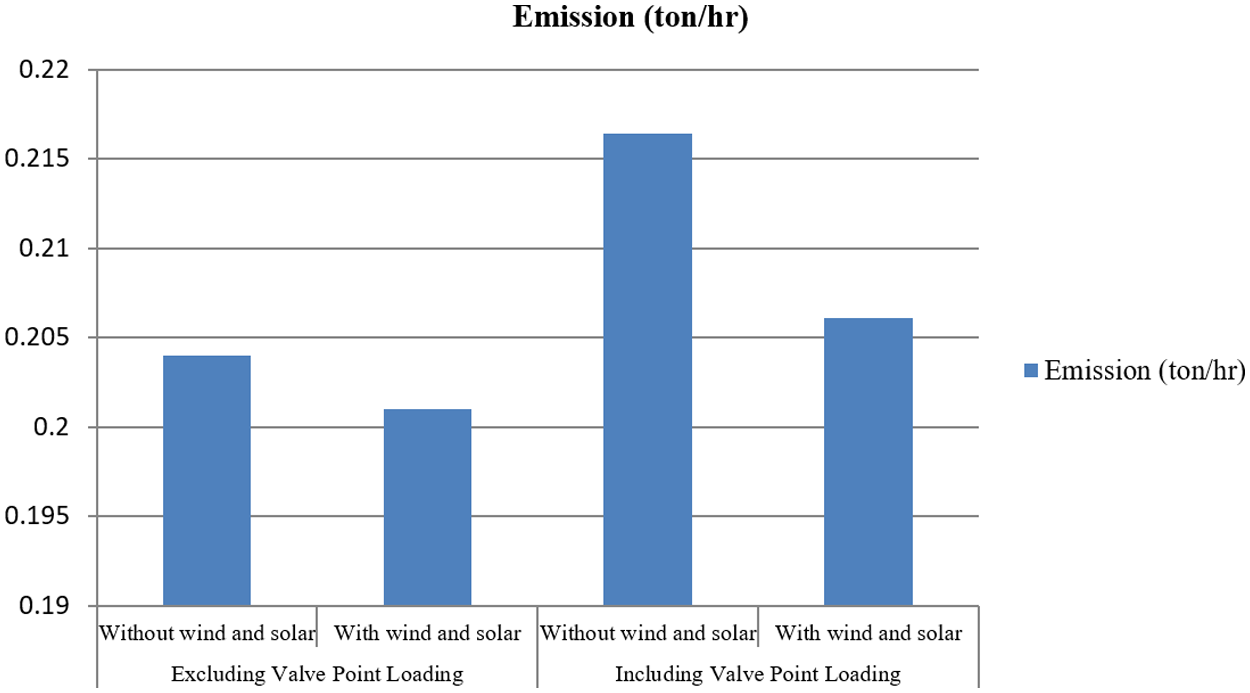
Figure 7: Emission in ton/hr in CEED-SMO
Solar irradiation and wind power are also used in this study, which is available 24 h a day. In Tab. 6, the combined 24 h CEED result is shown for wind and solar energy. Buses 4 and 7 are equipped with wind turbines. The total wind power injected is 1366 kW in order to diminish the fuel costs and emissions.
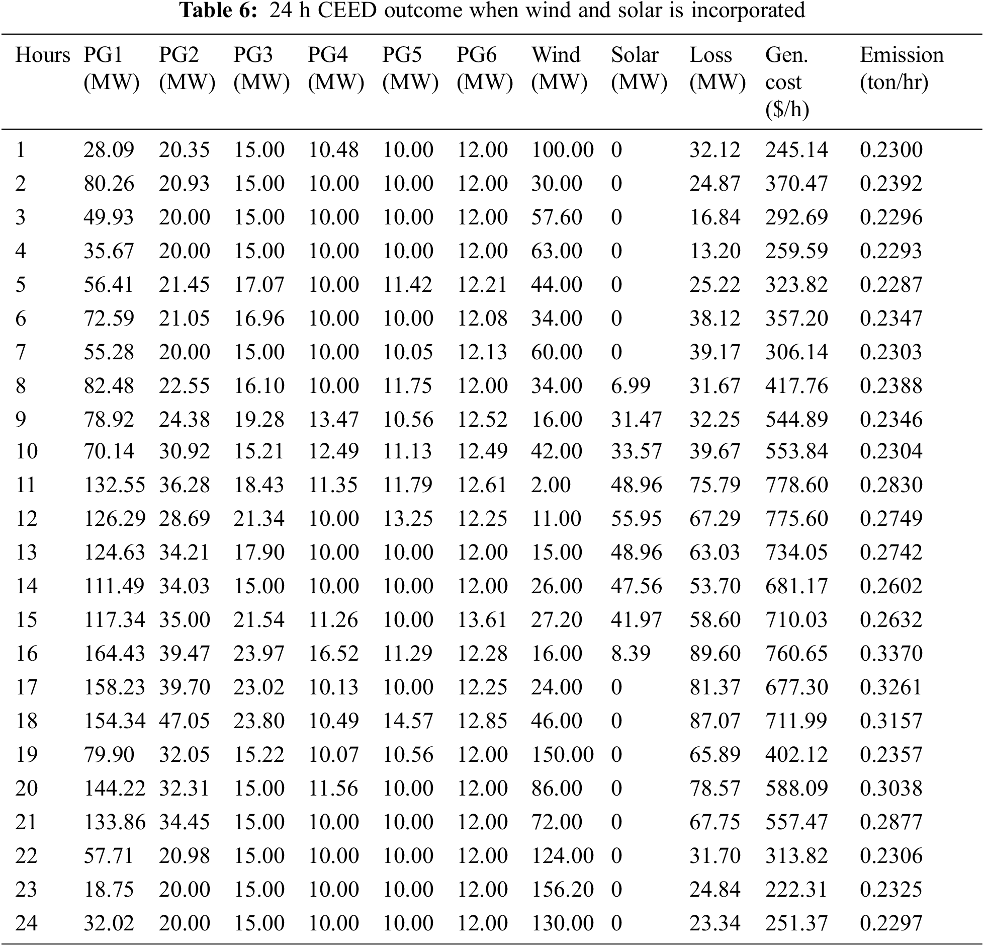
Fig. 8 depicts the incorporation of wind power into a power grid. At the 11th hour, wind power generation is 34MW, and at the 23rd hour, it is 156.20MW. From the figure, it shows that the wind power generation is excellent from the 18th hour. As wind is a natural occurrence, the wind velocity will vary throughout the course of 24 h. In this simulation, a single day is analyzed together with its wind pattern and power infusion.
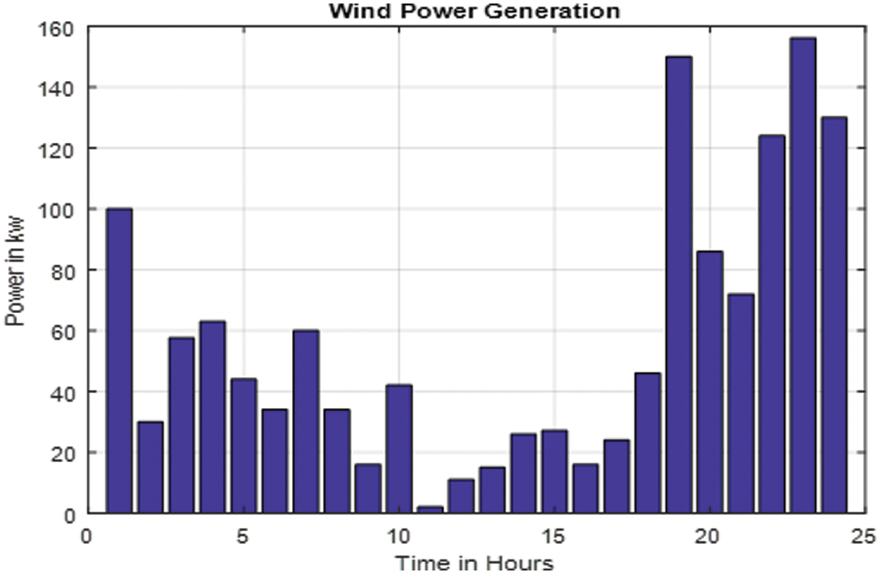
Figure 8: Wind power injection
The solar power perforation in the power system is depicted in Fig. 9. The buses 14, 15, and 21 are powered by solar panels. It explains the pattern of 24 h solar power generation. The figure clearly demonstrates that the solar power is generated from 8th hr to 16th hr as the solar energy generation is extreme only at noon hours.
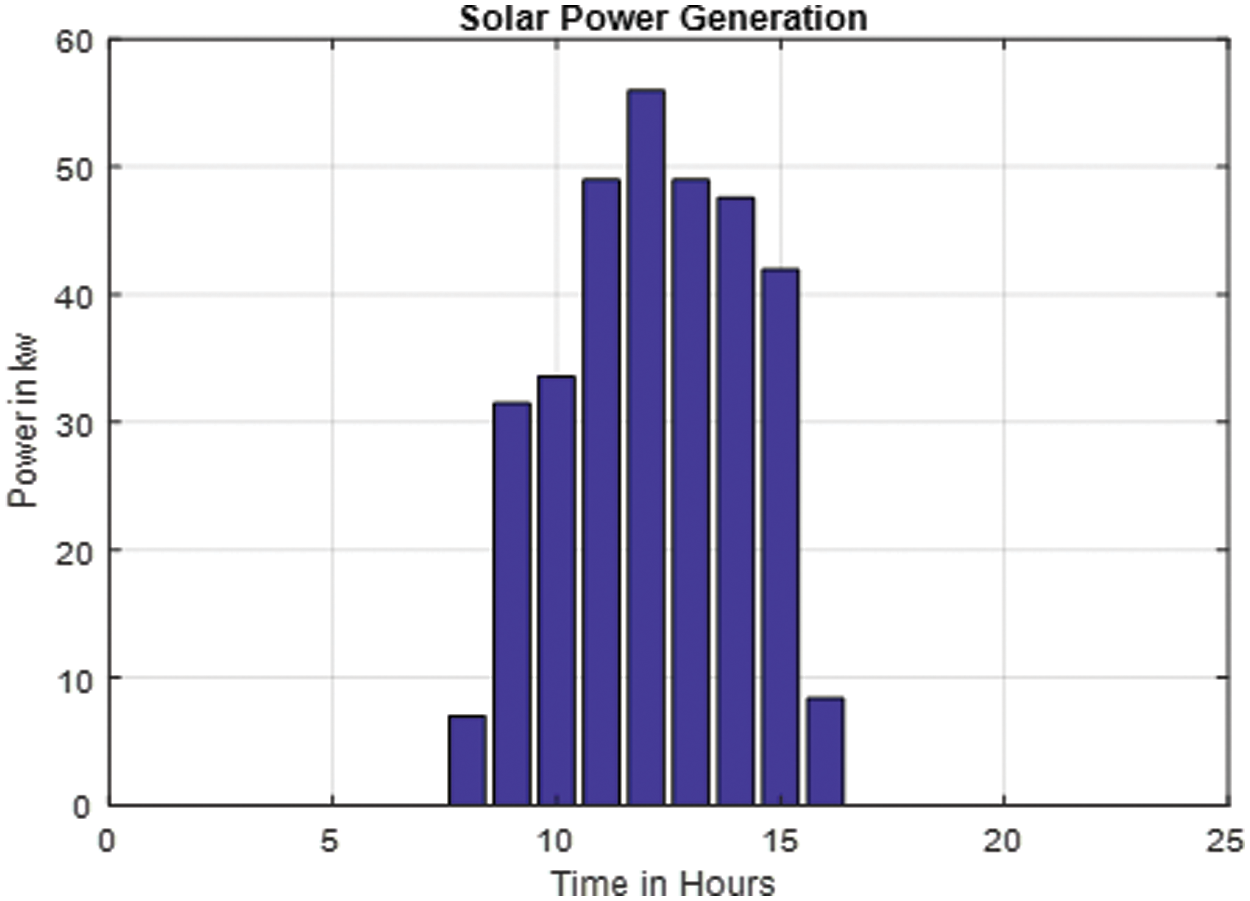
Figure 9: Solar power injection
The estimated voltage magnitudes of all 30 buses, are within the minimum (0.95 per unit) and maximum limitations (1.05 per unit). The voltage limit equation is thus met. The IEEE 30 bus standard test scenario employs four transformers. Within the limits of the provided objective function, the smart SMO algorithm determined the best transformer tap point.
Fig. 10 depicts the power production of thermal, wind, and solar generators for the allocated demand over a 24-hour period. Thermal generators meet the majority of the power demand in this figure. Renewable energy sources such as wind and solar power are being considered. Wind power is incorporated throughout the day based on wind speed or availability, whereas solar power is only exploited to the extreme around midday. The enclosures of renewable energies will also reduce generating costs and emissions.
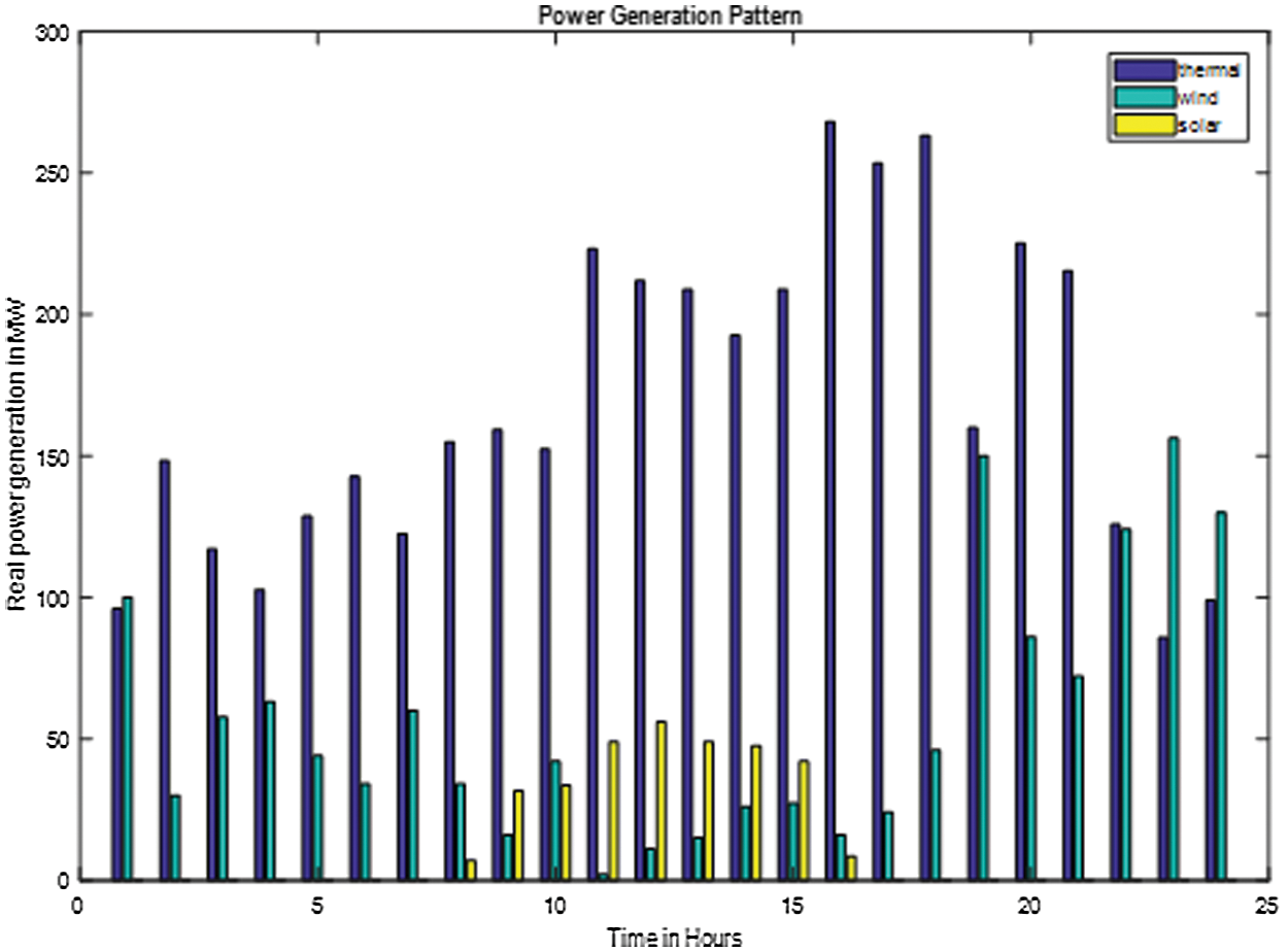
Figure 10: Power generation of thermal, wind and solar generators
Fig. 11 depicts the power demand in the power system throughout a 24-hour period. The active and reactive power demands are 283.4 MW and 126.2 MVAR, respectively.
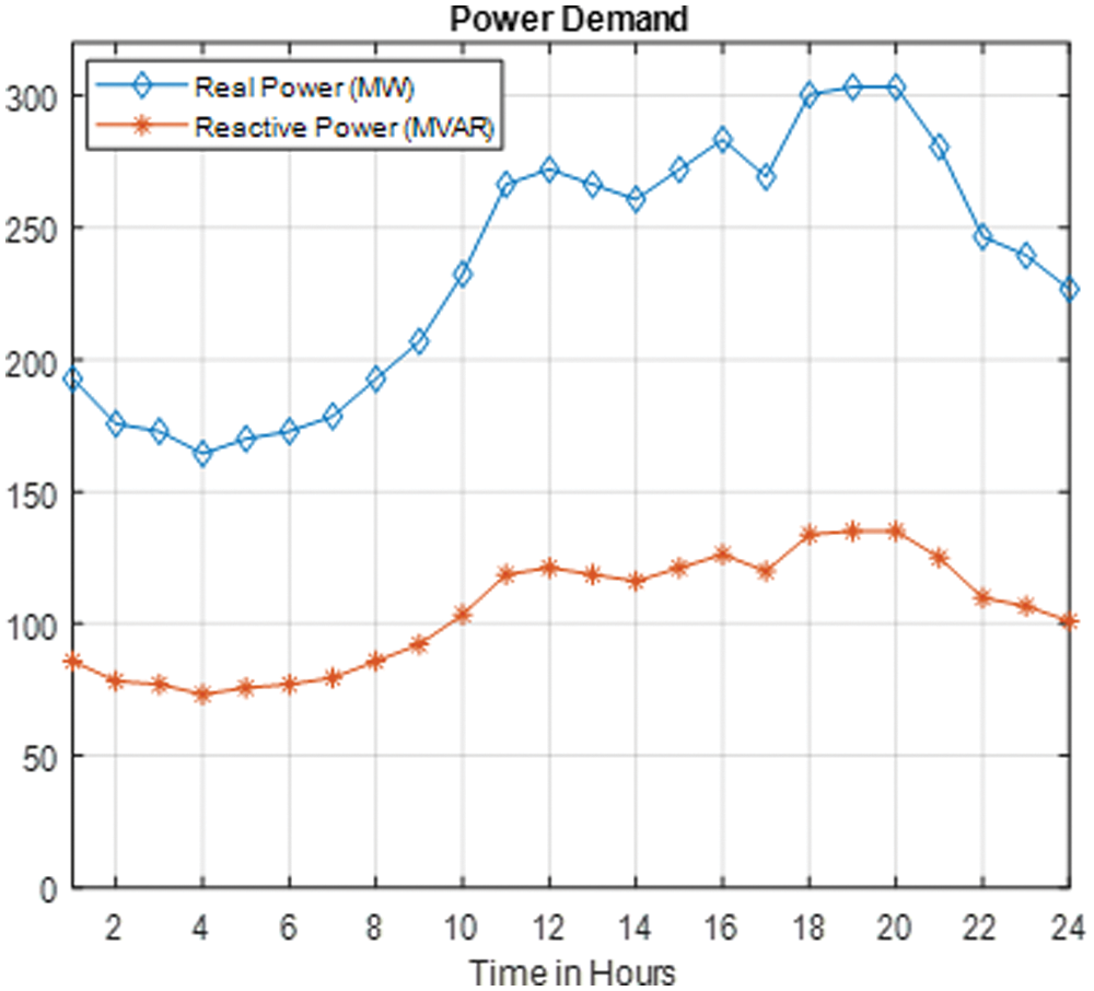
Figure 11: Power demand in the power system for 24 h
In this paper, the spider monkey optimization algorithm is used to unravel CEED with and without valve point loading. A single objective function is created by combining the cost of generation with the reduction of emissions. An IEEE standard test scenario is used to validate the proposed algorithm. When constraints are taken into account, the results show that the proposed SMO method is preferable in terms of achieving optimal results. The spider monkey optimization algorithm has produced excellent convergence properties when compared to other methods. Wind power and solar power are being recognized as renewable energies. Solar and wind power are used when they are available, and dedicated thermal generators are used to meet the remaining net demand. After the wind and solar power is included along with the thermal generating unit, 22.19% of generating cost is reduced without valve point loading and 28.49% of cost is reduced with valve point loading. Similarly 1.47% of emission is reduced without valve point loading and 4.76% of emission is reduced with valve point loading. This method reduces the cost and emissions of the power system’s generation. The initial population selection is crucial for the most optimal solution, which is one of SMOIA’s drawbacks. The mutation process isn’t available, and there are only a few search alternatives. Although a larger population demands more time to find the ideal solution, the recommended SMO approach handles the CEED problem better and produces superior results when compared to previous algorithms. In future, hybrid metaheuristics can be designed to improve performance.
Funding Statement: The authors received no specific funding for this study.
Conflicts of Interest: The authors declare that they have no conflicts of interest to report regarding the present study.
1. P. Aravindhababu and K. R. Nayar, “Economic dispatch based on optimal lambda using radial basis function network,” International Journal of Electrical Power & Energy Systems, vol. 24, no. 7, pp. 551–556, 2002. [Google Scholar]
2. J. Nanda, L. Hari and M. L. Kothari, “Economic emission load dispatch with line flow constraints using a classical technique,” IEE Proceedings-Generation, Transmission and Distribution, vol. 141, no. 1, pp. 1, 1994. [Google Scholar]
3. D. Karthikaikannan and G. Ravi, “Optimal reactive power dispatch considering multi-type facts devices using harmony search algorithms,” Automatika, vol. 59, no. 3–4, pp. 311–322, 2018. [Google Scholar]
4. M. Jevtic, N. Jovanic and J. Radosavljevic, “Experimental comparisons of metaheuristic algorithms in solving combined economic emission dispatch problem using parametric and non-parametric tests,” Applied Artificial Intelligence, vol. 32, no. 9–10, pp. 845–857, 2018. [Google Scholar]
5. M. A. Abido, “Environmental/economic power dispatch using multi objective evolutionary algorithms,” IEEE Transactions on Power Systems, vol. 18, no. 4, pp. 1529–1537, 2003. [Google Scholar]
6. H. Bouzeboudja, A. Chaker, A. Alali and B. Naama, “Economic dispatch solution using a real coded genetic algorithm,” Acta Electrotechnica et Informatica, vol. 5, no. 4, pp. 1–5, 2005. [Google Scholar]
7. M. A. Abido, “A novel multiobjective evolutionary algorithm for environmental economic power dispatch,” Electric Power System Research, vol. 65, no. 1, pp. 71–81, 2003. [Google Scholar]
8. K. P. Wong and C. C. Fung, “Simulated annealing based economic dispatch algorithm,” IEE Proceedings C (Generation, Transmission and Distribution), vol. 140, no. 6, pp. 509, 1993. [Google Scholar]
9. W. M. Lin, F. S. Cheng and M. T. Tsay, “An improved tabu search for economic dispatch with multiple minima,” IEEE Transactions on Power Systems, vol. 17, no. 1, pp. 108–112, 2002. [Google Scholar]
10. J. Cai, X. Ma, L. Li, Y. Yang, H. Peng et al., “Chaotic ant swarm optimization to economic dispatch,” Electric Power System Research, vol. 77, no. 10, pp. 1373–1380, 2007. [Google Scholar]
11. J. B. Park, K. Lee, J. Shin and K. Y. Lee, “A particle swarm optimization for economic dispatch with non smooth cost functions,” IEEE Transactions on Power Systems, vol. 20, no. 1, pp. 34–42, 2005. [Google Scholar]
12. A. Bhattacharya and P. K. Chattopadhyay, “Hybrid differential evolution with biogeography-based optimization for solution of economic load dispatch,” IEEE Transactions on Power Systems, vol. 25, no. 4, pp. 1955–1964, 2010. [Google Scholar]
13. C. N. Ravi, G. Selvakumar and C. C. A. Rajan, “Hybrid real coded genetic algorithm-differential evolution for optimal power flow,” International Journal of Engineering and Technology, vol. 5, no. 4, pp. 3404–3412, 2013. [Google Scholar]
14. S. Bhongade and S. Agarwal, “Artificial bee colony algorithm for an optimal solution for combined economic and emission dispatch problem,” International Journal of Applied Power Engineering, vol. 5, no. 3, pp. 111–119, 2016. [Google Scholar]
15. X. S. Yang, “Flower polliination algorithm for global optimization,” in Int. Conf. on Unconventional Computing and Natural Computation, UCNC 2012: Unconventional Computation and Natural Computation, Lecture Notes in Computer Science, vol. 7445, Springer, Berlin, Heidelber, pp. 240–249, 2012. [Google Scholar]
16. C. Shilajaa and K. Ravi, “Implementation of flower pollination algorithm for optimal power flow,” Journal of Electrical Engineering, vol. 17, no. 2, pp. 332, 2017. [Google Scholar]
17. R. Kathiravan and R. P. K. Devi, “Optimal power flow model incorporating wind, solar and bundled solar-thermal power in the restructured Indian power system,” International Journal of Green Energy, vol. 14, no. 11, pp. 934–950, 2017. [Google Scholar]
18. A. F. Ali, “An improved spider monkey optimization for solving a convex economic dispatch problem,” Nature-Inspired Computing and Optimization, vol. 10, pp. 425–448, 2017. [Google Scholar]
19. A. S. Tomar, H. M. Dubey and M. Pandit, “Combined economic emission dispatch using spider monkey optimization,” Advanced Engineering Optimization Through Intelligent Techniques, vol. 949, pp. 809–818, 2019. [Google Scholar]
20. S. Kumar, A. Nayyar and N. G. Nguyen, “Hyperbolic spider monkey optimization algorithm,” Recent Advances in Computer Science and Communications, vol. 13, no. 1, pp. 35–42, 2020. [Google Scholar]
 | This work is licensed under a Creative Commons Attribution 4.0 International License, which permits unrestricted use, distribution, and reproduction in any medium, provided the original work is properly cited. |