DOI:10.32604/iasc.2023.027703
| Intelligent Automation & Soft Computing DOI:10.32604/iasc.2023.027703 | |
| Article |
Modeling of Optimal Deep Learning Based Flood Forecasting Model Using Twitter Data
1Department of Computer Science and Engineering, RMK College of Engineering and Technology, Chennai, 601 206, India
2Department of Computer Science and Engineering, Saveetha Engineering College, Chennai, 602 106, India
*Corresponding Author: G. Indra. Email: indrav24@gmail.com
Received: 24 January 2022; Accepted: 02 March 2022
Abstract: A flood is a significant damaging natural calamity that causes loss of life and property. Earlier work on the construction of flood prediction models intended to reduce risks, suggest policies, reduce mortality, and limit property damage caused by floods. The massive amount of data generated by social media platforms such as Twitter opens the door to flood analysis. Because of the real-time nature of Twitter data, some government agencies and authorities have used it to track natural catastrophe events in order to build a more rapid rescue strategy. However, due to the shorter duration of Tweets, it is difficult to construct a perfect prediction model for determining flood. Machine learning (ML) and deep learning (DL) approaches can be used to statistically develop flood prediction models. At the same time, the vast amount of Tweets necessitates the use of a big data analytics (BDA) tool for flood prediction. In this regard, this work provides an optimal deep learning-based flood forecasting model with big data analytics (ODLFF-BDA) based on Twitter data. The suggested ODLFF-BDA technique intends to anticipate the existence of floods using tweets in a big data setting. The ODLFF-BDA technique comprises data pre-processing to convert the input tweets into a usable format. In addition, a Bidirectional Encoder Representations from Transformers (BERT) model is used to generate emotive contextual embedding from tweets. Furthermore, a gated recurrent unit (GRU) with a Multilayer Convolutional Neural Network (MLCNN) is used to extract local data and predict the flood. Finally, an Equilibrium Optimizer (EO) is used to fine-tune the hyperparameters of the GRU and MLCNN models in order to increase prediction performance. The memory usage is pull down lesser than 3.5 MB, if its compared with the other algorithm techniques. The ODLFF-BDA technique’s performance was validated using a benchmark Kaggle dataset, and the findings showed that it outperformed other recent approaches significantly.
Keywords: Big data analytics; predictive models; deep learning; flood prediction; twitter data; hyperparameter tuning
Natural flooding is the most common type of disaster [1]. Unlike stagnant water discharge, which occurs on occasion in poorly constructed communities, a big flood disaster frequently causes substantial property damage and, most of the time, leads in the loss of human life. This is significant because of the decrease in performance in predicting the calamity earlier. Regardless of the origin, a flood was usually unanticipated and nearly overwhelming for the relevant organisation and common people who had adequately prepared for the disasters [2]. Despite recent advancements in computerised flood prediction systems, it has remained primarily focused on current precipitation, as monitored by rain gauges or rain stations. Typically, these facilities are owned by comparable companies or meteorological departments [3]. In addition, due of the expensive cost of maintenance and installation, they are only found in a few areas. As a result, it is difficult to precisely predict floods or determine precipitation, particularly in areas lacking this capability [4]. To address this issue, precipitation in this area is typically estimated by interpolation or extrapolation from existing rain stations. Because of the small number of these stations, findings in one location may not be a true representation of others. As a result, evaluated precipitation was insufficient to create an accurate projection [5].
The flood prediction model is critical for extreme event management and hazard assessment. Strong prediction adds significantly to policy recommendations and analysis, additional evacuation modelling, and water resource management techniques. As a result, the importance of new methods for long-and short-term predictions of hydrological and flood events is highly highlighted in order to limit the consequences [6]. However, due to the dynamic nature of weather conditions, flood occurrence location and lead time forecast is becoming increasingly advanced. As a result, today’s principal flood prediction model includes several simplified assumptions and is mostly data-specific [7]. As a result, various techniques, such as empirical black box, event-driven, stochastic, deterministic, continuous, hybrids, lumped, and distributed, are used to simulate the complicated numerical depiction of physical processes and basin behaviours like model.
The drawbacks of statistical and physically based methods outlined above stimulate the employment of innovative data-driven techniques, such as machine learning (ML). Another reason for the model’s appeal is because it mathematically formulates the nonlinearity of the flood, relying purely on previous information and without knowledge of fundamental physical processes [8]. Data-driven prediction of artificial intelligence (AI) is used for generating patterns and regularities, which allow easier implementation with lower computational costs, fast testing, training, assessment, and validation, and superior performance than less complicated and physical models. Over the previous two decades, the progressive development of the ML approach has demonstrated its appropriateness for flood prediction with a reasonable rate of outperforming traditional methods.
Traditional intelligence approaches, such as deep learning (DL), could meet the difficulties of size and complexity. Once applied to ML, this technique may handle non-linearity and complexity without the requirement to comprehend the core procedures. In compared to the physical model, the computation intelligence model performs better, is faster, and requires fewer computer resources [9]. In recent decades, computational intelligence models have outperformed physical and statistical methodologies for flood prediction and modelling. Time series prediction and classification are potential flood modelling techniques inside the ML method [10]. Fuzzy-neuro system and artificial neural network are two categorization systems used in flood prediction (ANN). Flood classification with this computing intelligence approach comprises automatic feature extraction from time-series data, where the various layers in the DL algorithm allow for the recognition of trends and patterns in nonlinear data without pre-processing.
This research provides an Optimal Deep Learning-based Flood Forecasting model with Big Data Analytics (ODLFF-BDA) using Twitter data in a big data environment. The ODLFF-BDA technique comprises data pre-processing to convert the input tweets into a usable format. In addition, a Bidirectional Encoder Representations from Transformers (BERT) model is used to generate emotive contextual embedding from tweets. Furthermore, an equilibrium optimizer (EO) with Gated Recurrent Unit (GRU) and Multilayer Convolutional Neural Network (MLCNN) is employed to extract local information and anticipate the flood. The experimental result analysis of the ODLFF-BDA technique is validated against a benchmark Kaggle dataset, and the findings are evaluated in a variety of ways.
Löwe et al. [11] investigated how the DL approach might be structured to optimise the forecast of 2D maximal water depth maps in urban pluvial flood occurrences. A neural network (NN) system is trained to exploit patterns in topographical and hyetograph data in order to predict flood depth for observed spatial locations and rain events that were not included in the training data sets. A NN model is widely used for image segmentation (U-NET) is used. Puttinaovarat et al. [12] provided an adopting ML technique for flood prediction based on the merging of hydrological, meteorological, crowdsource, and geospatial big data. A sophisticated learning method drove data intelligence. According to objective and subjective evaluation, the proposed method is capable of anticipating flood episodes that occur in certain places.
Tehrany et al. [13] tested the hypothesis that adding a conditioning factor to a data set used in river flood modelling improves the final susceptibility mapping results. The two powerful ML approaches, DT and SVM, were used to evaluate spatial relationships among flood conditioning elements and estimate their significance level in order to map flood-prone locations. Dodangeh et al. [14] presented an integrated flood susceptibility prediction model based on multi-time resampling methods, bootstrapping (BT) and Random Subsampling (RS) models, and ML approaches such as Boosted Regression Tree (BRT), Multi-variate Adaptive Regression Splines (MARS), and Generalised Additive Model (GAM). The BT and RS approaches provide ten rounds of data resampling for model validation and learning.
Using ensemble models, Khalaf et al. [15] developed a strategy for predicting water levels as well as flood severity. This method takes advantage of recent improvements in IoT and ML for autonomous flood analysis, which could be useful in preventing natural disasters. Neelakandan et al. [16] look into DL approaches for predicting gauge height and evaluating the associated uncertainty. The models are developed and validated using gauge height data from the Meramec River at Valley Park, Missouri. The analysis indicated that the DL methodology outperforms the statistical and physical methods currently in use when providing data in 15-minute increments rather than six-hour intervals. Divyabharathi et al. [17] created a DL technique for predicting stream flow that combines the strong predicting power of Back Propagation Neural Network (BPNN) with the feature representation capacity of SAE. To improve the nonlinearity simulation capability, first use K-means clustering to categorise each data set into multiple classes. Following that, multiple SAE-BP models are modified to simulate the various data classes.
Interventionary studies involving animals or humans, and other studies that require ethical approval, must list the authority that provided approval and the corresponding ethical approval code.
Fig. 1 depicts the overall operation of the ODLFF-BDA approach. The Hadoop Map Reduce tool is used to handle large amounts of data. The ODLFF-BDA approach relies heavily on pre-processing to convert tweets into usable formats. Then, BERT is used to convert the word tokens in the real tweets into word embeddings. The GRU model is then used to capture the order information and long-term dependencies in a sequence of words. Furthermore, the MCNN model is used as a feature extractor to derive patterns from the GRU model’s embedding. The results of the MCNN model are fed into the detection layer, which determines whether or not the prediction is correct. The EO-based hyperparameter tuning approach is also used in this study to improve the predicted outcomes.
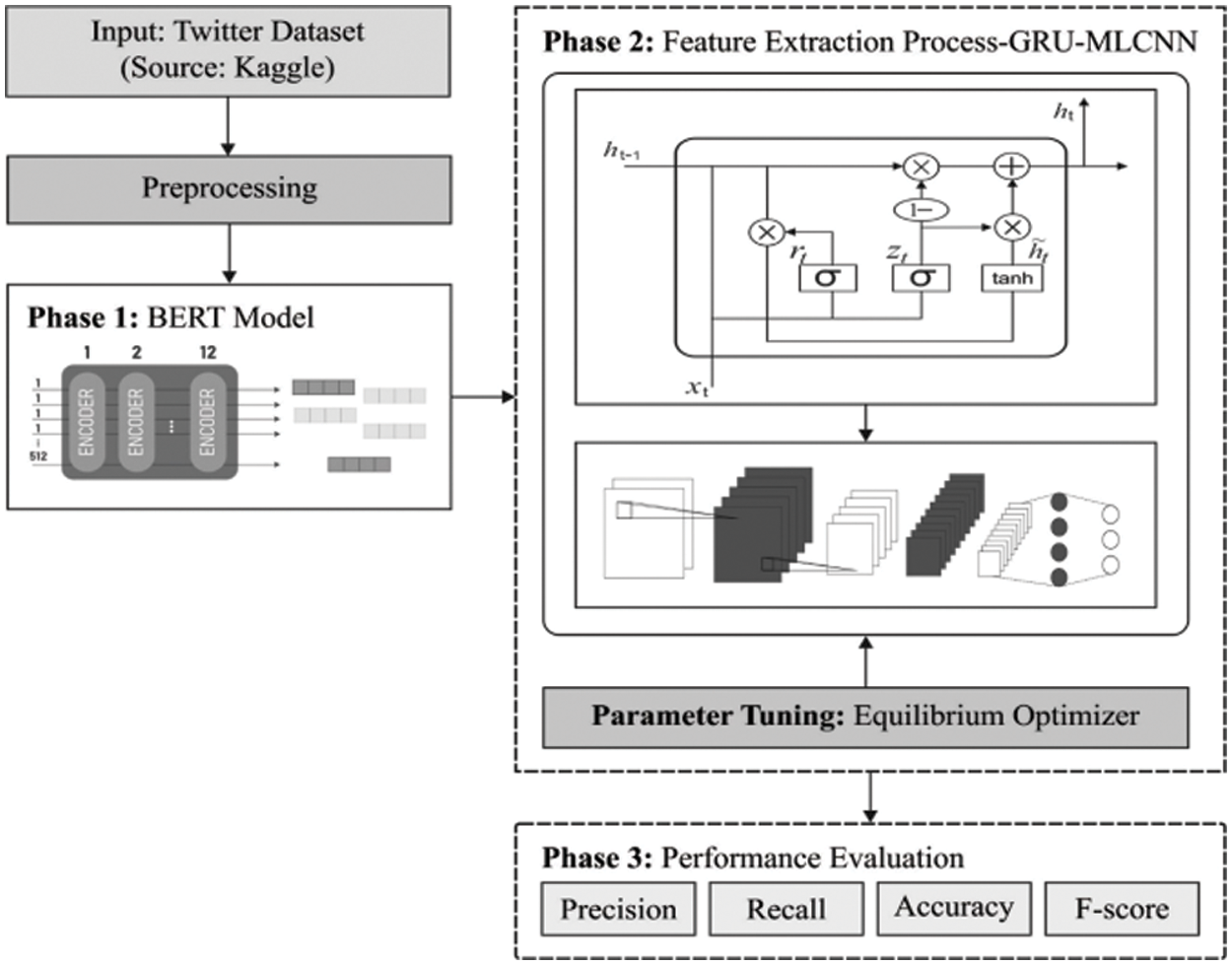
Figure 1: Overall process of ODLFF-BDA technique
MapReduce (MR) is a simplified programming model that also serves as an effective distributed scheduling model. Programming is much easier under the Cloud Computing platform. The platform can manage cluster treatment, including scalability and reliability. Application developers are required to focus on the application itself. The two core computing components are “Map” and “Reduce.” Fig. 2 displays the Hadoop framework [18].
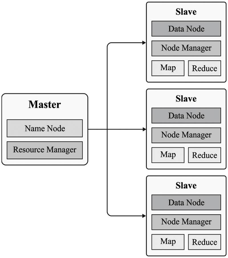
Figure 2: Hadoop architecture
Big data is segmented into unconnected chunks by the Map software and spread to a large number of computers to process, resulting in distributed computing. The results of this computer are then outputted and summarised by the Reduce model. (Key, value) pairs are used to represent data.
A Map function is used to extract data from text, and this pair is sent to an intermediate temporary space specified by MR [19]. The key/value pair is grouped according to the key via an intermediate procedure performed by the Map function. Then, given a complete list, a Reduce function determines the maximum number.
In most cases, the input tweets contain noise that must be eliminated. As a result, data pre-processing is used to remove punctuation marks, emojis, and hashtags. For example, “# it’s chill. :)” can be converted into “it’s chill.” Following that, a few preliminary conversions occur by altering “We’ve” to “We have” in order to create an effective word separation in a sentence. Finally, each message is tokenized in order to generate a set of word sequences as input to the learning process.
BERT is an attention-based language approach that uses a stack of encoded and decoded Transformers to learn textual material. BERT [20] is a well-known modern language modelling structure. Its universal ability is that it may be modified to other downstream tasks dependent on what is required, such as Named-entity recognition or relation extraction, question answering, or sentiment analysis (SA). Because the core structure was trained on largely large text corpora, the parameter of the mostly interior layer of structure is locked. Individuals in the outermost layer adjust to duties, and on that basis, so called finetuning is implemented. Furthermore, the BERT framework employs two unique tokens: [SEP] for segmentation separation and [CLS] for classification, which are used as primary input tokens to some classifier, demonstrating the entire order and obtaining a resultant vector of similar size as hidden size H. So, the outcome of transformer, for instance, the last hidden state of primary token utilized as input is represented as vector C∈R^H. The vector C has been utilized as input of last FC classifier layer. To provide the parameter matrix W∈R^KxH of classifier layer, where K the amount of categories, the probability of all categories P are computed by softmax function as:
The transformer is the base of BERT. Assume that x and y as order of sub-words attained from 2 sentences. The [CLS] token has placed before x, but the [SEP] token was placed afterward combined with x and y. Approximately E is the embedded function and LN refers the normalized layer, the embedded was attained with:
Following that, the embedded is passed through the M transformer block. It is possible to prove that [21], using the Feed Forward layer, the element wise Gaussian Error Linear Unit (GELU) activation functions, and the Multi Heads Self Attention (MHSA) function from all transformer blocks
where
Conversely, from all attention heads, it can be valid that:
where
3.4 GRU and MCNN Based Feature Extraction
GRU is a variant of the Long short-term memory (LSTM) network. It gains from the RNN method in that it automatically obtains features and successfully processes long-term dependent data. It is carried out efficiently to estimate short-term traffic [22]. Fig. 3 depicts the cell infrastructure of GRU networks in their concealed state, and it may be clearly related to LSTM. Intuitively, an input and forget gate from LSTM are merged as a reset gate from GRU that defines for combining a novel input data in the past. Another gate in GRU is known as the upgrade gate, and it defines numerous data in the preceding time that is saved to the present time. As a result, the GRU is one gate less connected to the LSTM. Furthermore, the cell and hidden state from LSTM are concatenated to form a single hidden state from GRU. It can be modified to produce GRU networks with different parameters, a faster learning speed, and less information required for efficiently generalising the model. GRU’s computation equation is as follows:
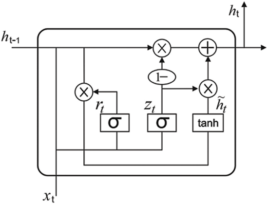
Figure 3: Structure of GRU model
Eqs. (13) and (14) demonstrate that updating gate zn and reset gate rn were computed from GRU neurons. Wz signifies the weight of zn, Wr implies the weight of rn, and 0 stands for the sigmoid functions. The innermost time
Input, output, and multiple hidden layers are all part of the Modified Convolutional Neural Network (MCNN). MCNN’s hidden layer is typically composed of a convolution layer, a normalisation layer, a pooling layer, and a fully connected (FC) layer. The convolution layer applies a convolutional function to the input and then transfers the result to the next layer [24]. The convolutional neural network responds to visual stimuli by following the responses of individual neurons. The convolutional function provides a solution by reducing the number of parameters for improving network depth, but it still uses a large number of parameters. The normalisation layer normalises the activation as well as gradient propagation with the network, which simplifies the optimal issue of the trained network [25,26]. The batch normalisation layer, which is used in conjunction with the convolution layer and non-linearity, is used to accelerate network training and reduce sensitivity to network initialization [27–29]. The pooling layer combines the outcomes of neuron clusters from one layer with a single neuron from the next layer. Max pooling, on the other hand, uses the maximum value in all clusters of neurons from the preceding layer [30,31]. The FC layer incorporates the picture classification feature. The final FC layer’s resultant size parameter was equal to the number of classes in the target data.
The EO is used to optimally modify the hyperparameters in the GRU and MCNN models. In 2020, the notion of single objective EO was introduced [32]. The EO was relying on dynamic mass balancing on a control volume where it applies a mass balance formula. The mass balance formula seeks the system’s equilibrium states. During the initialization step, EO employs a particle group in which all of the particles define the vector of concentration that includes the solution to the problem. It can be stated as follows:
In which,
The concentration update enables EO to equally balance exploitation and exploration
In which
It and Max−it represent the present and the maximal amount of iterations, and a2 denotes a constant for controlling the capacity to exploit. Other parameters a1, is utilized for improving exploration and exploitation.
The rate of generation is denoted as G that enhances exploitation.
In which,
Here, the arbitrary number is represented as r1 and r2 and differs between zero and one. The vector
The value of V is equivalent to one.
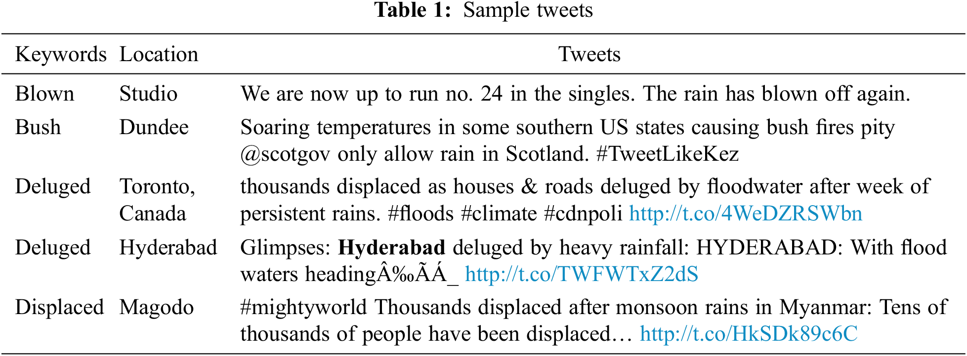
The Twitter dataset is used for experimental validation of the ODLFF-BDA approach in the Kaggle competition [33,34]. The dataset contains 10876 cases, 4692 of which are classified as positive (disaster) and 6184 as negative (not disaster). Tab. 1 contains a selection of tweets from the Kaggle dataset.
The classification result analysis of the ODLFF-BDA technique on flood prediction under varied batch sizes (BS) and epochs is presented in Tab. 2. The ODLFF-BDA technique produced precision of 98.57%, recall of 97.58%, accuracy of 98.08%, and F score of 98.88 percent with BS of 16 and 100 epochs. Furthermore, after 300 epochs, the ODLFF-BDA approach achieved a precision of 98.33%, a recall of 98.38 percent, an accuracy of 98.38%, and a F score of 98.32%. After 500 epochs, the ODLFF-BDA approach achieved a precision of 98.69%, a recall of 97.66%, an accuracy of 97.89%, and a F score of 98.20%. The ODLFF-BDA technique produced a precision of 97.45%, a recall of 97.78%, an accuracy of 97.64%, and a F score of 98.12% with BS of 32 and 100 epochs. After 300 epochs, the ODLFF-BDA technique achieved a precision of 97.66%, a recall of 97.95%, an accuracy of 97.84%, and a F score of 98.14%. Furthermore, after 500 epochs, the ODLFF-BDA system has a precision of 97.06%, a recall of 97.33%, an accuracy of 97.14%, and a F score of 98.60%.
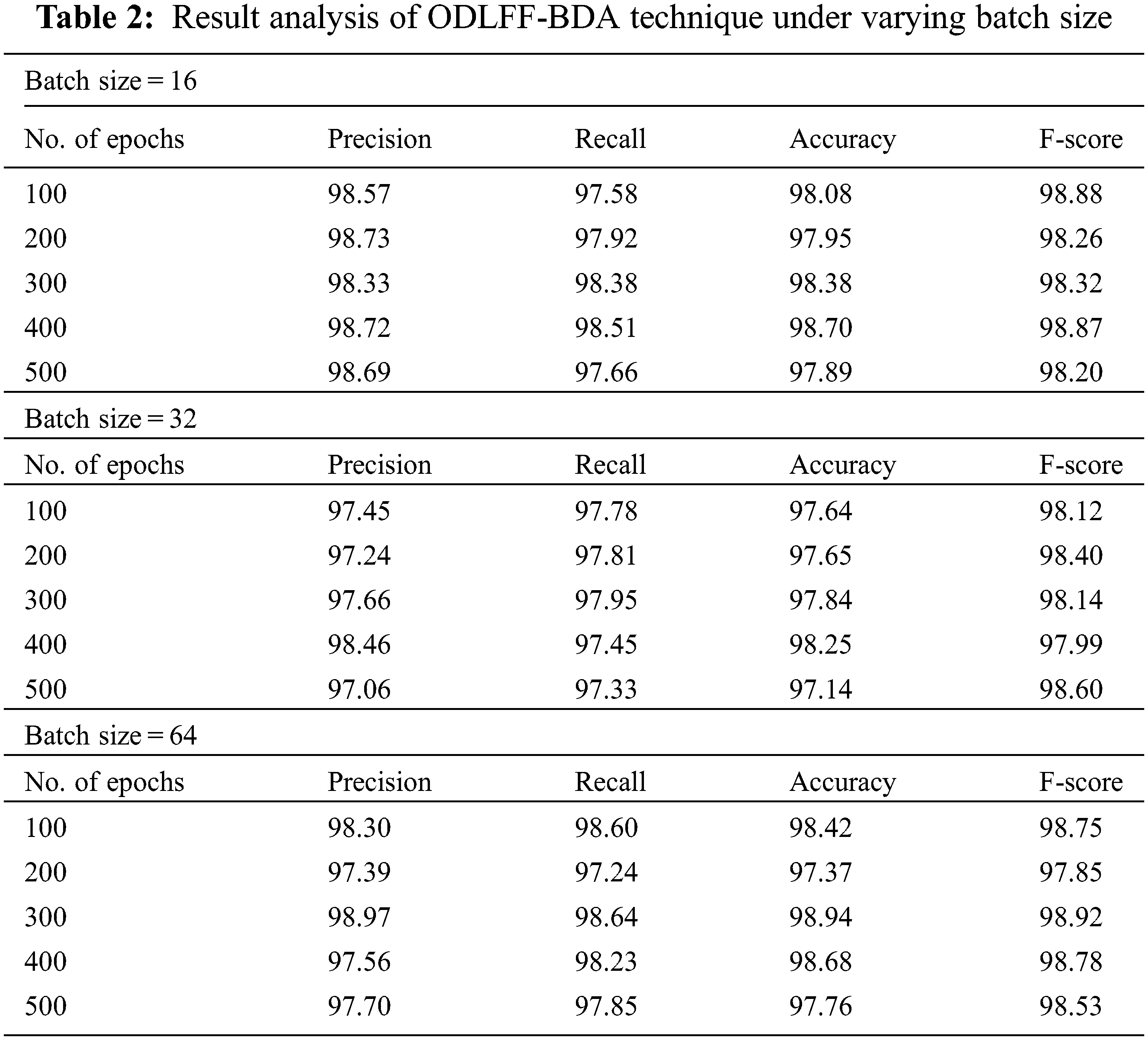
Similarly, with BS of 64 and 100 epochs, the ODLFF-BDA methodology has resulted to prec_n of 98.30%, reca_l of 98.60%, accu_y of 98.42%, and F_score of 98.75%. Likewise, under 300 epochs, the ODLFF-BDA algorithm has achieved prec_n of 98.97%, reca_l of 98.64%, accu_y of 98.94%, and F_score of 98.92%. Furthermore, under 500 epochs, the ODLFF-BDA algorithm has reached prec_n of 97.70%, reca_l of 97.85%, accu_y of 97.76%, and F_score of 98.53%.
The accuracy analysis of the ODLFF-BDA technique on the test dataset is depicted in Fig. 4. The results demonstrated that the ODLFF-BDA technique improved performance with greater training and validation accuracy. It is apparent that the ODLFF-BDA system has achieved higher validation accuracy than training accuracy.
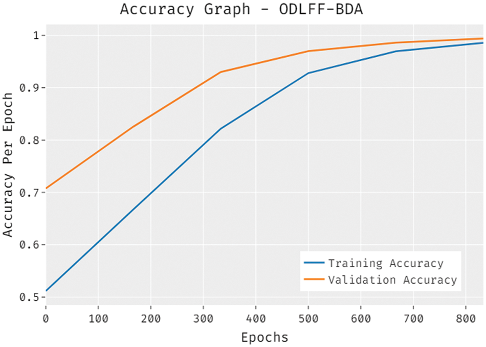
Figure 4: Accuracy graph analysis of ODLFF-BDA technique
The loss analysis of the ODLFF-BDA approach on the test dataset is depicted in Fig. 5. The results demonstrated that the ODLFF-BDA strategy produced a competent outcome with lower training and validation loss. The ODLFF-BDA method is said to have provided lower validation loss compared to training loss.
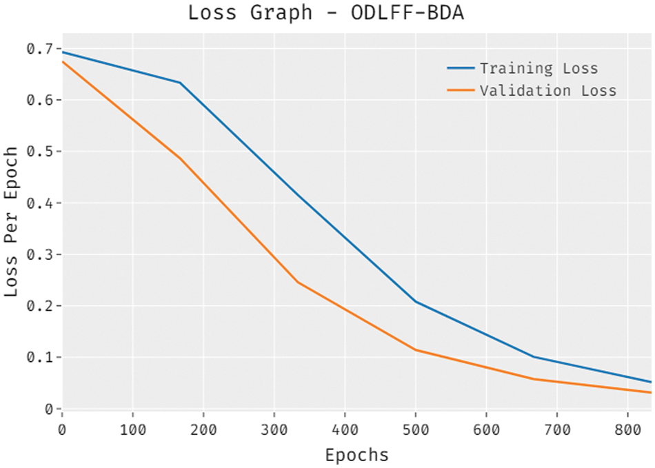
Figure 5: Loss graph analysis of ODLFF-BDA technique
Tab. 3 [35] compares the results of the ODLFF-BDA technique to those of other approaches. The precision, recall, and F1-score analysis of the ODLFF-BDA technique using modern approaches is depicted in Fig. 6. The results revealed that the CNN and BiLSTM-CNN techniques performed ineffectively with the lowest precision, recall, and F1-score values. Furthermore, the S-BiLSTM-CNN, DT, RF, SVM, and ANN approaches all achieved significantly higher precision, recall, and F1-score values. However, the ODLFF-BDA technique outperformed the other techniques with greater precision, recall, and F1-score of 98.97%, 98.64%, and 98.92%, respectively.
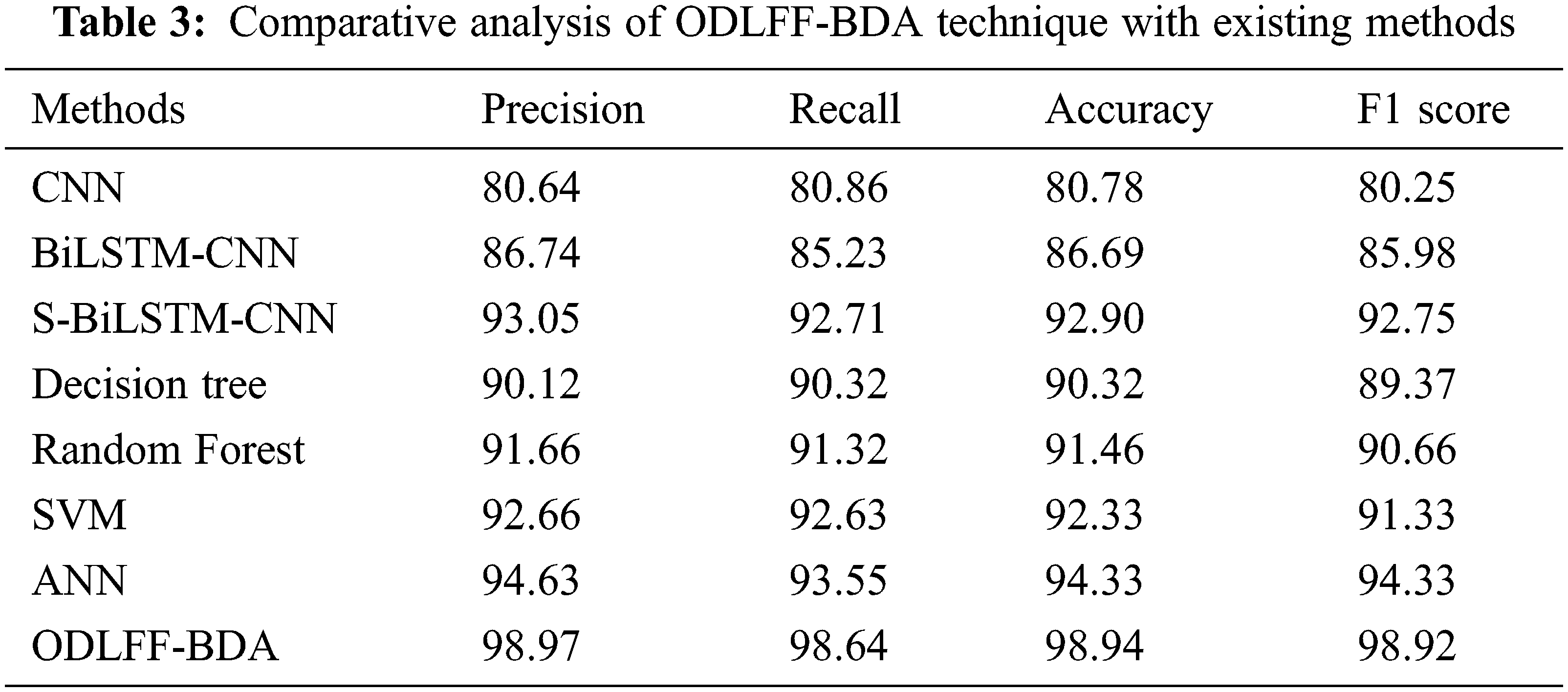
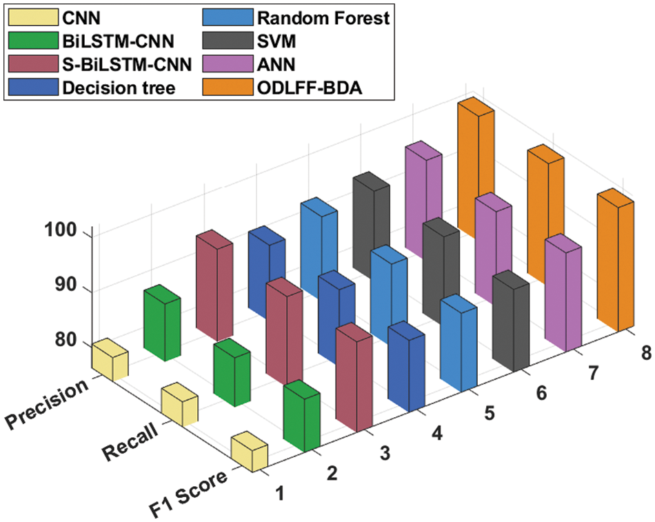
Figure 6: Comparative analysis of ODLFF-BDA technique with existing approaches
The accuracy analysis of the ODLFF-BDA approach with modern techniques is depicted in Fig. 7. According to the findings, the CNN and BiLSTM-CNN models performed ineffectively, with the lowest accuracy values. Additionally, the S-BiLSTM-CNN, Decision Tree, Random Forest, SVM, and ANN approaches have achieved significantly higher levels of accuracy. The ODLFF-BDA methodology, on the other hand, outperformed the other methods, with a maximum accuracy of 98.94%.
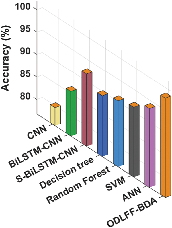
Figure 7: Accuracy analysis of ODLFF-BDA technique with recent methods
Tab. 4 and Fig. 8 present a brief computation time (CT) comparison of the ODLFF-BDA technique with contemporary approaches. According to the graph, the DT model produced worse results with a CT of 8.34 min. In keeping with this, the RF and CNN models achieved marginally better performance with CTs of 7.51 and 7.01 min, respectively. Following that, the BiLSTM-CNN, S-BiLSTM-CNN, SVM, and ANN approaches achieved moderately closer CT of 6.07, 6.00, 6.31, and 6.34 min, respectively. The ODLFF-BDA approach, on the other hand, yielded a maximum CT of 5.17 min.
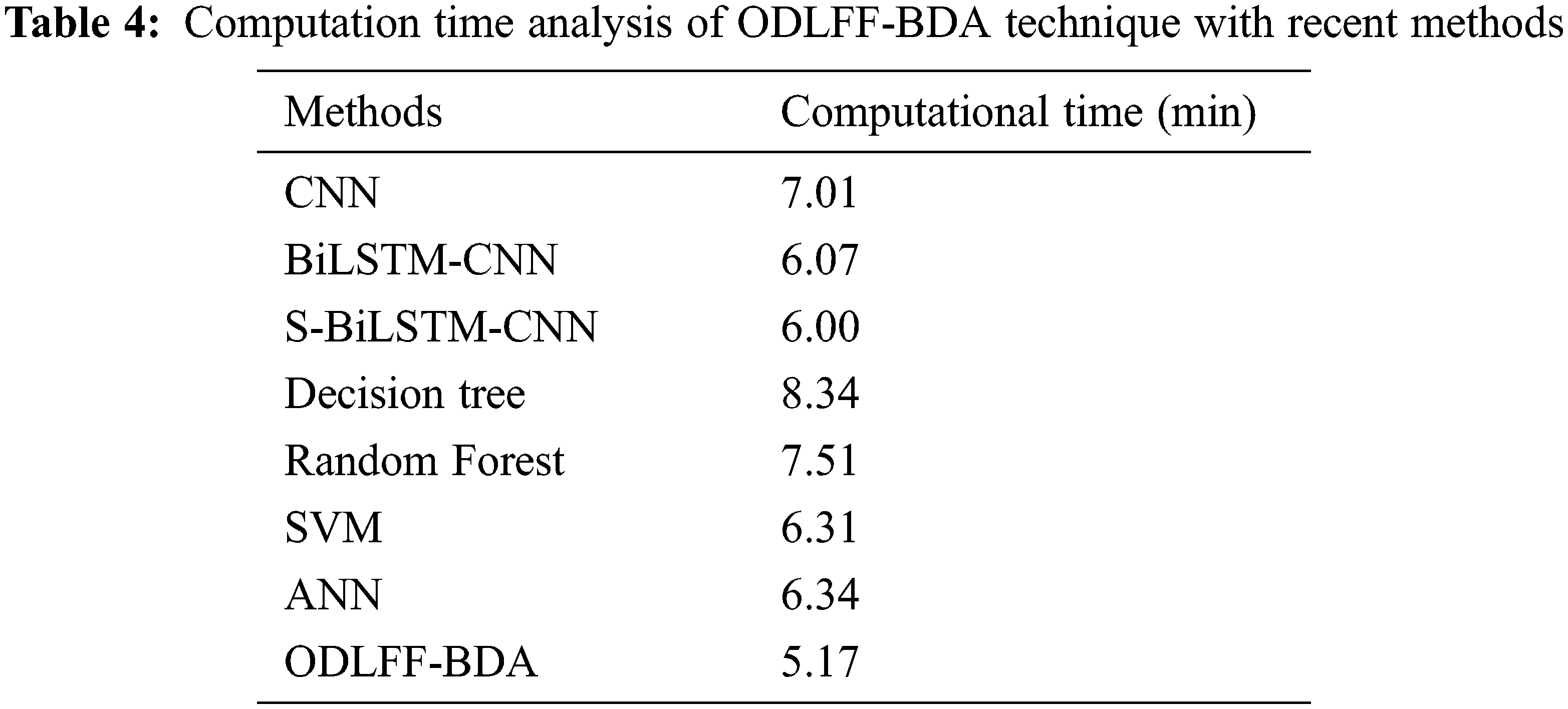
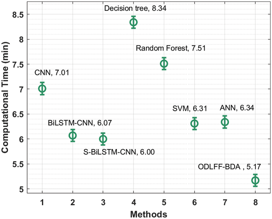
Figure 8: C T analysis of ODLFF-BDA technique with existing algorithms
Tab. 5 and Fig. 9 present a detailed memory use (MU) study of the ODLFF-BDA strategy using contemporar y techniques. The graph showed that the DT system produced the worst results, with a MU of 46722.15 Mb. In keeping with this, the RF and CNN approaches produced slightly higher results, with MUs of 43923.07 Mb and 40774.12 Mb, respectively. Furthermore, the BiLSTM-CNN, S-BiLSTM-CNN, SVM, and ANN algorithms achieved somewhat closer MU of 36575.50 Mb, 35626.62 Mb, 37975.04 Mb, and 39374.58 Mb, respectively. Finally, the ODLFF-BDA approach resulted in a higher MU of 33426.55 Mb.
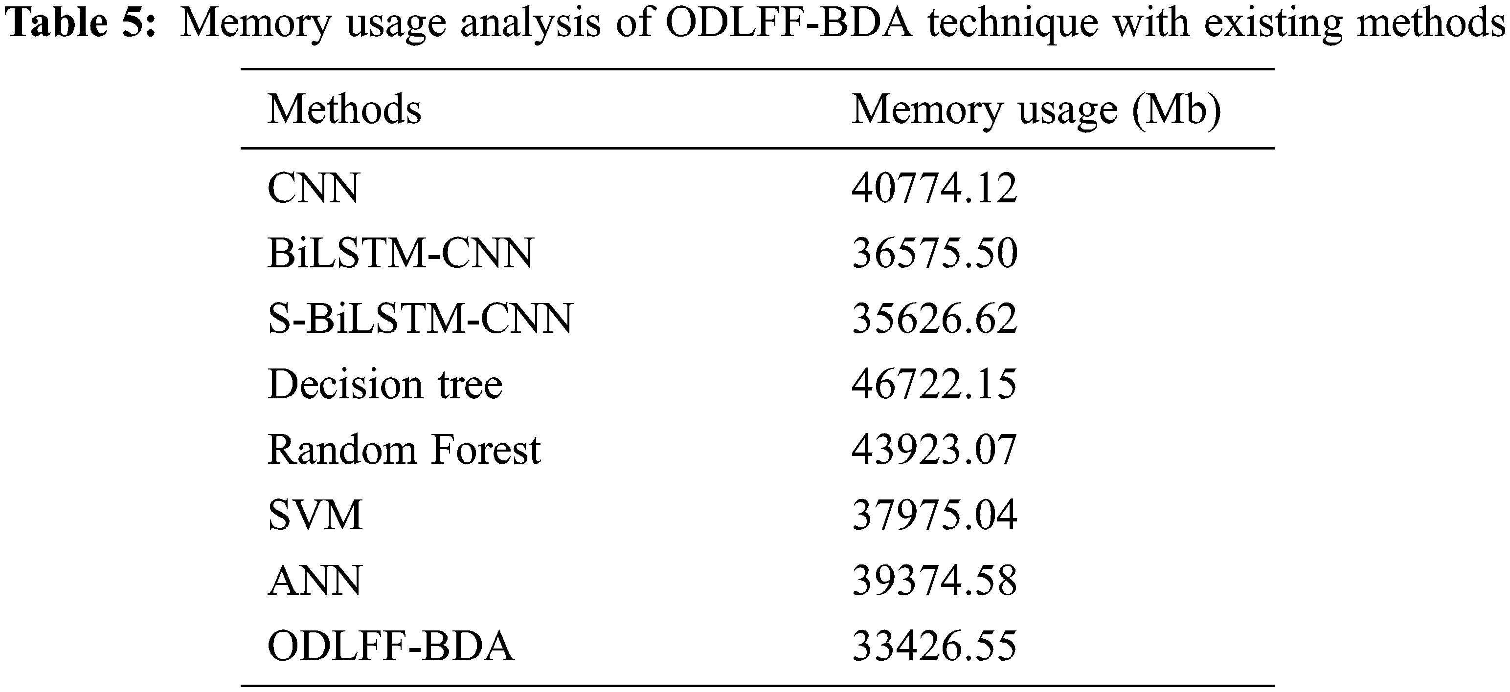
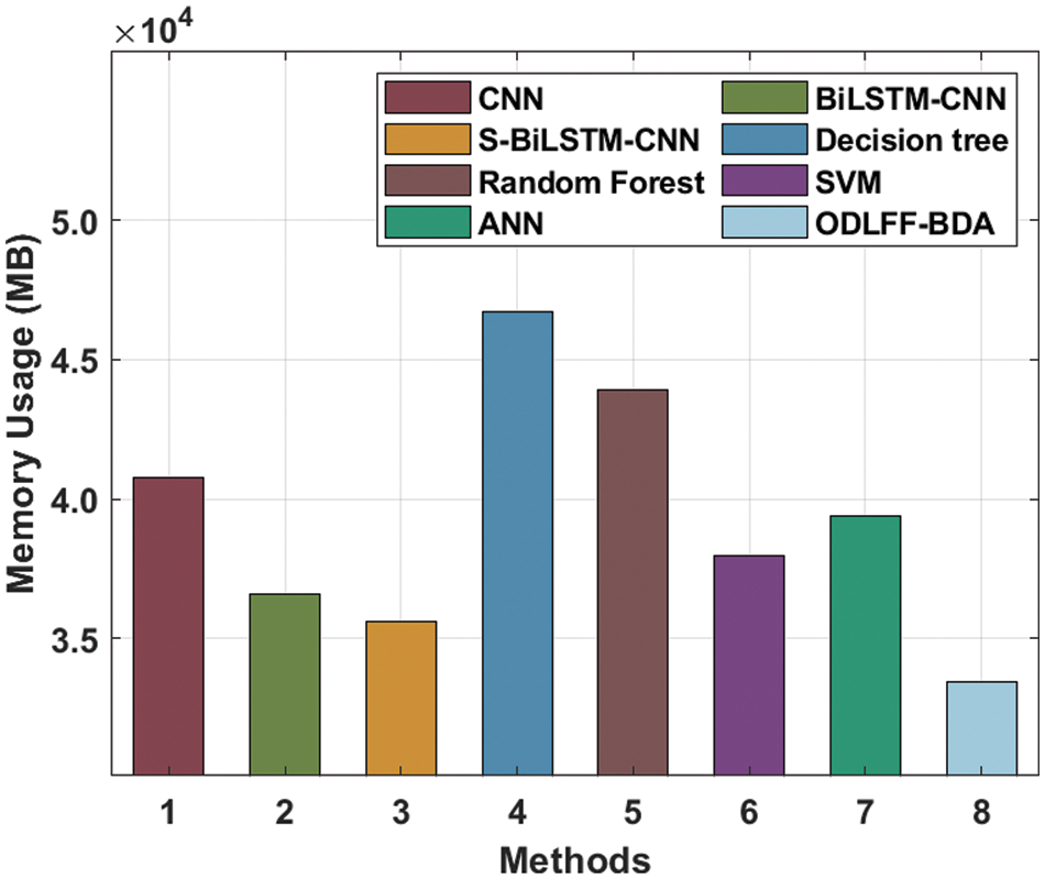
Figure 9: MU analysis of ODLFF-BDA technique with recent methods
The above-mentioned tables and graphs illustrate that the ODLFF-BDA technique outperforms the other techniques.
In this paper, a new ODLFF-BDA technique for predicting floods using Twitter data in a big data context is presented. Pre-processing, BERT-based word embedding, MCNN-based feature extraction, and softmax (SM)-based classification comprise the ODLFF-BDA approach. The BERT model is used to generate attentive hidden states, while the MCNN model is utilised to extract feature vectors. In addition, a typical detection head accepts the input as a concatenation of the produced features and sends it to an FC layer, which is followed by an SM layer, to produce the prediction outcomes. The EO-based hyperparameter tuning approach is also used in this study to improve the predicted outcomes. The experimental result analysis of the ODLFF-BDA technique is validated against a benchmark Kaggle dataset, and the findings are scrutinised in a number of ways. The broad comparative investigation found that the ODLFF-BDA approach outperformed the most recent approaches.
Funding Statement: The authors received no specific funding for this study.
Conflicts of Interest: The authors declare that they have no conflicts of interest to report regarding the present study.
1. D. T. Nguyen and S. T. Chen, “Real-time probabilistic flood forecasting using multiple machine learning methods.” Water, vol. 12, no. 3, pp. 1–13, 2020. [Google Scholar]
2. S. K. Sood, R. Sandhu, K. Singla and V. Chang, “IoT, big data and HPC based smart flood management framework,” Sustainable Computing: Informatics and Systems, vol. 20, no. 1, pp. 102–117, 2020. [Google Scholar]
3. A. Mosavi, P. Ozturk and K. W. Chau, “Flood prediction using machine learning models: Literature review,” Water, vol. 10, no. 11, pp. 1–12, 2018. [Google Scholar]
4. V. D. Ambeth Kumar, S. Malathi, K. Abhishek and C. V. Kalyana, “Active volume control in smart phones based on user activity and ambient noise,” Sensors, vol. 20, no. 15, pp. 1–17, 2020. [Google Scholar]
5. X. H. Le, H. V. Ho, G. Lee and S. Jung, “Application of long short-term memory neural network for flood forecasting,” Water, vol. 11, no. 7, pp. 1–10, 2019. [Google Scholar]
6. X. Xu, X. Zhang, H. Fang, R. Lai, Y. Zhang et al., “A Real-time probabilistic channel flood-forecasting model based on the Bayesian particle filter approach,” Environmental Modelling & Software, vol. 88, no. 1, pp. 151–167, 2018. [Google Scholar]
7. J. Noymanee and T. Theeramunkong, “Flood forecasting with machine learning technique on hydrological modeling,” Procedia Computer Science, vol. 156, no. 1, pp. 377–386, 2018. [Google Scholar]
8. I. F. Kao, Y. Zhou, L. C. Chang and F. J. Chang, “Exploring a long short-term memory based encoder-decoder framework for multi-step-ahead flood forecasting,” Journal of Hydrology, vol. 583, no. 10, pp. 1–18, 2020. [Google Scholar]
9. M. Moishin, R. C. Deo, R. Prasad, N. Raj and S. Abdulla, “Designing deep-based learning flood forecast model with ConvLSTM hybrid algorithm,” IEEE Access, vol. 9, no. 12, pp. 50982–50993, 2021. [Google Scholar]
10. L. Chen, N. Sun, C. Zhou, J. Zhou, Y. Zhou et al., “Flood forecasting based on an improved extreme learning machine model combined with the backtracking search optimization algorithm,” Water, vol. 10, no. 10, pp. 1–15, 2018. [Google Scholar]
11. R. Löwe, J. Böhm, D. G. Jensen, J. Leandro and S. H. Rasmussen, “U-FLOOD–Topographic deep learning for predicting urban pluvial flood water depth,” Journal of Hydrology, vol. 603, no. 1, pp. 1–13, 2021. [Google Scholar]
12. S. Puttinaovarat and P. Horkaew, “Flood forecasting system based on integrated big and crowdsource data by using machine learning techniques,” IEEE Access, vol. 8, no. 8, pp. 5885–5905, 2020. [Google Scholar]
13. M. S. Tehrany, S. Jones and F. Shabani, “Identifying the essential flood conditioning factors for flood prone area mapping using machine learning techniques,” Catena, vol. 175, no. 2, pp. 174–192, 2019. [Google Scholar]
14. E. Dodangeh, B. Choubin, A. N. Eigdir, N. Nabipour, M. Panahi et al., “Integrated machine learning methods with resampling algorithms for flood susceptibility prediction,” Science of the Total Environment, vol. 705, no. 2, pp. 1–14, 2020. [Google Scholar]
15. M. Khalaf, H. Alaskar, A. J. Hussain, T. Baker, Z. Maamar et al., “IoT-Enabled flood severity prediction via ensemble machine learning models,” IEEE Access, vol. 8, no. 8, pp. 70375–70386, 2020. [Google Scholar]
16. S. Neelakandan and A. Ramanathan, “Social media network owings to disruptions for effective learning,” Procedia Computer Science, vol. 172, no. 5, pp. 145–151, 2020. [Google Scholar]
17. S. Divyabharathi and S. Rahini, “Large scale optimization to minimize network traffic using MapReduce in big data applications,” in Int. Conf. on Computation of Power, Energy Information and Communication (ICCPEIC), India. pp. 193–199, April 2016. [Google Scholar]
18. K. Balasaravanan and C. Saravanakumar, “An enhanced security measure for multimedia images using hadoop cluster,” International Journal of Operations Research and Information Systems, vol. 12, no. 3, pp. 1–8, 2021. [Google Scholar]
19. S. Manikandan, S. Sambit and D. Sanchali, “An efficient technique for cloud storage using secured de-duplication algorithm,” Journal of Intelligent & Fuzzy Systems, vol. 42, no. 2, pp. 2969–2980, 2021. [Google Scholar]
20. J. Devlin, M. Chang, K. Lee and K. Toutanova, “BERT: Pre-training of deep bidirectional transformers for language understanding,” in Proc. of the 2019 Conf. of the North American Chapter of the Association for Computational Linguistics: Human Language Technologies, NAACL-HLT 2019, Minneapolis, MN, USA, pp. 2–7, 2019. [Google Scholar]
21. P. V. Rajaram, “Intelligent deep learning based bidirectional long short term memory model for automated reply of e-mail client prototype,” Pattern Recognition Letters, vol. 152, no. 12, pp. 340–347, 2021. [Google Scholar]
22. M. Pota, M. Ventura, R. Catelli and M. Esposito, “An effective BERT-based pipeline for twitter sentiment analysis: A case study in Italian,” Sensors, vol. 21, no. 1, pp. 133–145, 2021. [Google Scholar]
23. L. Kuan, Z. Yan and W. Xin, “Short-term electricity load forecasting method based on multilayered self-normalizing GRU network,” in Proc. of the 2017 IEEE Conf. on Energy Internet and Energy System Integration (EI2), Beijing, China, pp. 1–5, 2017. [Google Scholar]
24. B. Jaishankar, V. Santosh, S. P. Aditya Kumar, P. Ibrahim and N. Arulkumar, “Blockchain for securing healthcare data using squirrel search optimization algorithm,” Intelligent Automation & Soft Computing, vol. 32, no. 3, pp. 1815–1829, 2022. [Google Scholar]
25. C. Pretty Diana Cyril, J. Rene Beulah, A. Harshavardhan and D. Sivabalaselvamani, “An automated learning model for sentiment analysis and data classification of twitter data using balanced CA-SVM,” Concurrent Engineering Research and Applications, vol. 29, no. 4, pp. 386–395, 2020. [Google Scholar]
26. S. Neelakandan, “An automated exploring and learning model for data prediction using balanced ca-svm,” Journal of Ambient Intelligence and Humanized Computing, vol. 12, no. 5, pp. 4979–4990, 2020. [Google Scholar]
27. F. I. Chou, Y. K. Tsai, Y. M. Chen, J. T. Tsai and C. C. Kuo, “Optimizing parameters of multi-layer convolutional neural network by modeling and optimization method,” IEEE Access, vol. 7, no. 11, pp. 68316–68330, 2019. [Google Scholar]
28. D. Paulraj, “A gradient boosted decision tree-based sentiment classification of twitter data,” International Journal of Wavelets, Multiresolution and Information Processing, vol. 18, no. 4, pp. 1–21, 2020. [Google Scholar]
29. R. Chithambaramani and M. Prakash, “A cloud interoperability framework using i-anfis,” Symmetry, vol. 13, no. 2, pp. 1–14, 2021. [Google Scholar]
30. A. Rohit and S. Harinder, “Interpretable filter based convolutional neural network (IF-CNN) for glucose prediction and classification using PD-SS algorithm,” Measurement, vol. 183, no. 3, pp. 1–15, 2021. [Google Scholar]
31. R. R. Bhukya, B. M. Hardas and T. Ch., “An automated word embedding with parameter tuned model for web crawling,” Intelligent Automation & Soft Computing, vol. 32, no. 3, pp. 1617–1632, 2022. [Google Scholar]
32. L. Natrayan, B. T. Geetha, J. Rene Beulah and R. Sumathy, “IoT enabled environmental toxicology for air pollution monitoring using AI techniques,” Environmental Research, vol. 205, no. 8, pp. 1–12, 2022. [Google Scholar]
33. A. Faramarzi, M. Heidarinejad, B. Stephens and S. Mirjalili, “Equilibrium optimizer: A novel optimization algorithm,” Knowledge-Based Systems, vol. 191, no. 5, pp. 1–12, 2020. [Google Scholar]
34. C. Al-Atroshi, V. K. Nassa, B. Geetha et al. (2022). Deep Learning-Based Skin Lesion Diagnosis Model Using Dermoscopic Images. Intelligent Automation & Soft Computing, vol. 31, no. 1, pp. 621–634. [Google Scholar]
35. C. Ramalingam, “Addressing semantics standards for cloud portability and interoperability in multi cloud environment,” Symmetry, vol. 13, no. 2, pp. 1–17, 2021. [Google Scholar]
 | This work is licensed under a Creative Commons Attribution 4.0 International License, which permits unrestricted use, distribution, and reproduction in any medium, provided the original work is properly cited. |