DOI:10.32604/iasc.2023.028444
| Intelligent Automation & Soft Computing DOI:10.32604/iasc.2023.028444 | |
| Article |
Identification and Acknowledgment of Programmed Traffic Sign Utilizing Profound Convolutional Neural Organization
1Department of Networking and Communications, SRM Institute of Science and Technology, Kattankulathur, Chennai, 603203, India
2Department of Computer Science and Engineering, School of Engineering, Presidency University, Bengaluru, 560064, India
*Corresponding Author: P. Vigneshwaran. Email: vigneshwaranpandi1981@gmail.com
Received: 10 February 2022; Accepted: 20 March 2022
Abstract: Traffic signs are basic security workplaces making the rounds, which expects a huge part in coordinating busy time gridlock direct, ensuring the prosperity of the road and dealing with the smooth segment of vehicles and individuals by walking, etc. As a segment of the clever transportation structure, the acknowledgment of traffic signs is basic for the driving assistance system, traffic sign upkeep, self-administering driving, and various spaces. There are different assessments turns out achieved for traffic sign acknowledgment in the world. However, most of the works are only for explicit arrangements of traffic signs, for example, beyond what many would consider a possible sign. Traffic sign recognizable proof is generally seen as trying on account of various complexities, for example, extended establishments of traffic sign pictures. Two critical issues exist during the time spent identification (ID) and affirmation of traffic signals. Road signs are occasionally blocked not entirely by various vehicles and various articles are accessible in busy time gridlock scenes which make the signed acknowledgment hard and walkers, various vehicles, constructions, and loads up may frustrate the ID structure by plans like that of road signs. Also concealing information from traffic scene pictures is affected by moving light achieved by environment conditions, time (day-night), and shadowing. Traffic sign revelation and affirmation structure has two guideline sorts out: The essential stage incorporates the traffic sign limitation and the resulting stage portrays the perceived traffic signs into a particular class.
Keywords: Traffic sign; classifier; convolution neural network; image; vehicle
Modified traffic sign disclosure and affirmation is a captivating point concerning Personal Computers (PC) vision and is especially critical concerning independent vehicle advancement. To maintain road prosperity, it expects to play a significant role in front-line driver assistance systems and autonomous vehicles. Automatic Traffic Sign Detection and Recognition (ATSDR) is a constantly evolving topic to address, given the variety of rush hour jam signs and contrasting environmental variables exhibited in genuine road settings [1]. Furthermore, development relics contained in a live, very active congested video stream complicate disclosure and confirmation. The issue has been researched for a long period of time, and numerous solutions have been proposed. These techniques, in general, split into two sections: Traffic Sign Instantly recognizable proof and Traffic Sign Confirmation, and handle each one independently. Limiting zones in a picture that may include traffic signs are revealed in the revelation step, and these constrained areas are depicted in the affirmation step to convey sign types of establishments. The use of the deep convolution association method in Traffic Sign Area has shown significant improvements in image affirmation, partition, and thing recognition [2,3]. In any event, traffic signs account for below 3% of the picture in the peak period jam sign ID datasets. As a consequence, the thing to imagine extent addresses a significant difficulty in describing a model for dividing such small items. To plan truly meaningful relationships, the technique requires additional computer capacity and a large amount of data. Testing biological conditions has an effect on the image, making it insensitive to road conditions. The inconvenient conditions, along with the sign size objectives and the enormous volume of data needed to measure, make this extremely inconvenient [4]. Across all benchmarks, significant learning computations based on Convolutional Neural Connections have showed enormous performance in PC vision tasks like as picture confirmation, division, and article recognition. It’s also a good time to think about incorporating these tactics into ATSDR structures. Another stumbling block to properly using Convolutional Neural Networks (CNNs) to resolve this issue is the enormous amount of information necessary to plan genuinely meaningful associations [5]. To work with study in the field of Road Signs Interpretation and Affirmation, a massive number of photographs with substantial standards are used. Encoder-Decoder Designing is used to create the localizer, which is then followed by a Fully Convolutional Association that is powered by SegNet & U-Net Plan. There are two phases to the connection: a codec and a neural connection, which are linked using a residual learning technique. From the Cutoff points area detected by the Localizer [6], the Classifier component predicts the traffic sign. Images from the German Road Signs Areas Test Data and German Road Signs Affirmation Benchmark Dataset are used to create the Neural Associations (GTSRB). The GTSRB collection comprises almost 50,000 images divided into 432 categories. The GTSDB dataset contains 900 images that localizer modules use to detect and reduce traffic sign region limitations.
Convolutional neural networks have demonstrated significant advances in image recognition, segmentation, and object recognition when used to identify traffic signs. The localizer as well as the classifier, both of which are detailed below, are the two primary components of this research. A Transceiver framework [7] as well as a Fully Convolutional Neural System architectures are employed to produce the localizer. Multiple convolution frames, each with a handful of 3 * 3 or even more convolution layers, some type of batch normalization layer, and a ReLU activation layer, make up the encoder stage. In most cases, the encoder step is divided into two tiers. A pair of * 2 max-pooling functions are used to accomplish reduced sampling for everyone and every block. The best component’s individual index is noted so that it may be utilised throughout the up-sampling procedure. The number of feature stations grows by a factor of two with each down sampling step. The development of the subsequent decoder block has begun in earnest. At each level of decoding, the map is upward sampled by using a 2 * 2 up convolution. During up sampling, a duplicate of an element is created to the index saved from the relevant max - pooling of the decoder [8]. This up convolution reduces the feature map by half, which is then combined with the comparable convolution layer from the decoder. After the concatenation feature map has already been treated via two 3 * 3 convolution layers, a ReLU activation layer is added. A 1*1 convolution layer inside the final layer maps each component feature vector from the previous layers to two categories. When it happens, a Convolutional Neural Network is employed to boost the Encoder-Decoder Network’s performance. It is possible to predict the boundaries of 32 × 32 square images using the Encoder-Decoder, which are then scaled and created from the predicted bounds. The CNN style incorporates the VGG-16 design, which appears to be often used in image recognition applications. This picture is acquired by some other CNN [9] for law enforcement agencies road signs zones during a specific area. It’s made up of two interconnected layers, each with two serial 3 * 3 convolutions, a Relu layer, but at most one layer [10,11]. When each block of the algorithm is executed, a dropout layer with a probability of 0.25 is inserted. The characteristics are sent via two completely linked layers to induce at this point: the first, triggered by ReLU, has a concealed size of 1024 bits, while the other, triggered by SoftMax, has a concealed length of fifteen bits [12].
The major goal of our research is to construct a deep CNN for vehicle detection with the highest possible accuracy. Our proposed work’s second goal is to split the inputs into several modules in order to establish the path, determine the outside, classify the photos, and acquire the final result.
The paper holds the main objective of implementing a deep convolutional neural network for detection of traffic signs and achieving maximum accuracy. The predicted coordinates by the localizer module should be more accurate so that the intersection portion with the background is minimum. To label the images in the dataset more accurately and further analyze the dataset. To detect the image edges properly and extract features under critical challenging conditions. To implement VGG 16 Classification model approach in detection of traffic signs. To improve the accuracy of the classifier module by adding hyperparameters and adding more regularization parameters and dropout layers to the neural network module. Fig. 1 depicts the general architecture schematic for the proposed system. Path Extractor, Localizer, Boundary Extraction, and Classifier are the four modules that make up the suggested work.

Figure 1: Overall architecture diagram
Fig. 2 shows how we designed the Path Extractor technique to allow us to work on multiple features of traffic sign recognition at the same time. Thanks to Extractor Design, we may use different optimization algorithms at various stages of the pipeline. Neural networks excel at executing extremely precise tasks. As a consequence, we may take use of the strengths of various designs to increase the efficacy of one network while sacrificing the precision of others. Because Neural Models are produced in constrained equipment contexts, it is considerably easier to train multiple deep networks for each specific job rather than a single extremely deep network for the entire network.
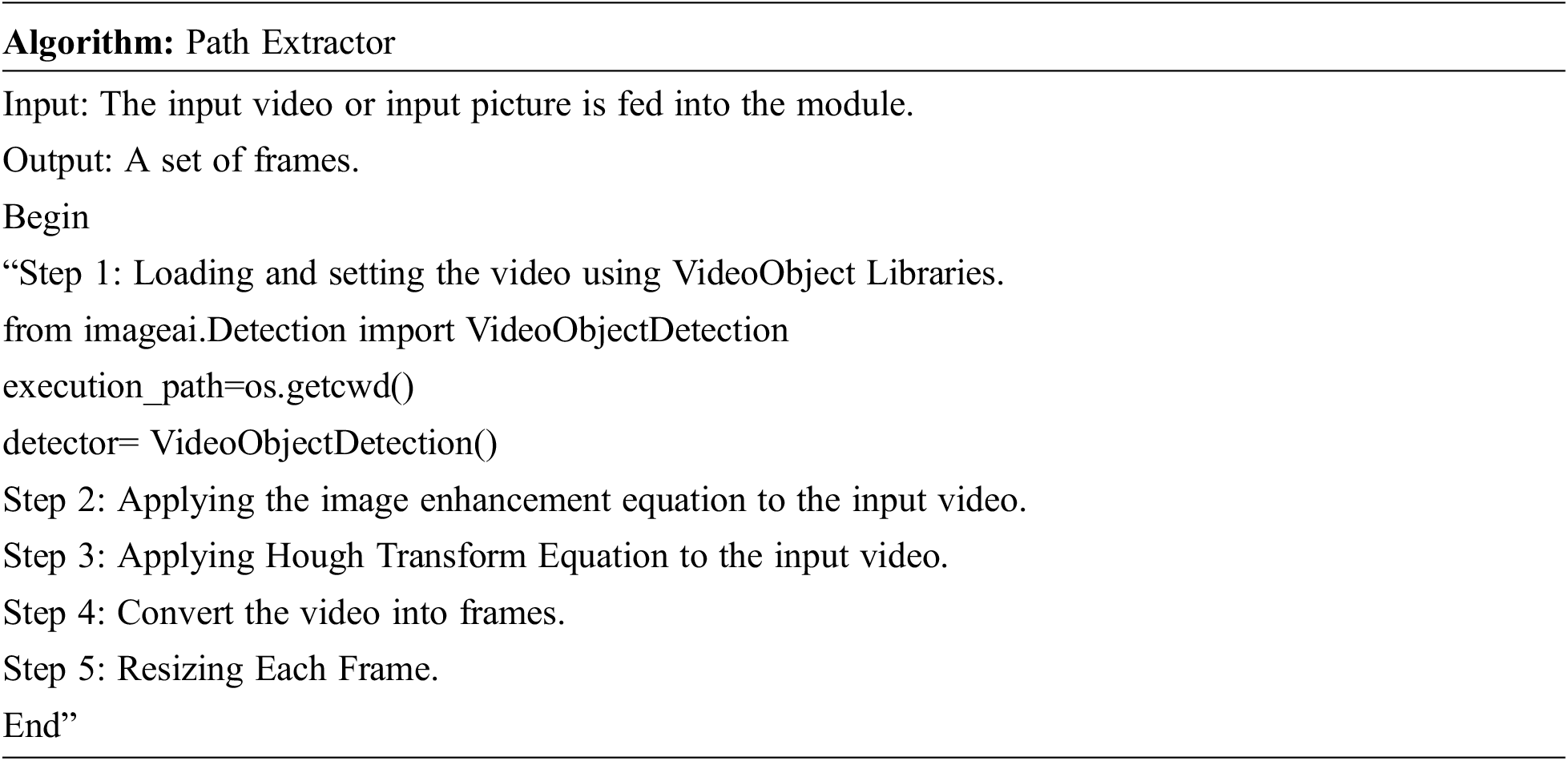

Figure 2: Path extractor module diagram
The Path Extractor Module involves generating a Stable set of frames, which are fed into the neural network for boundary detection.
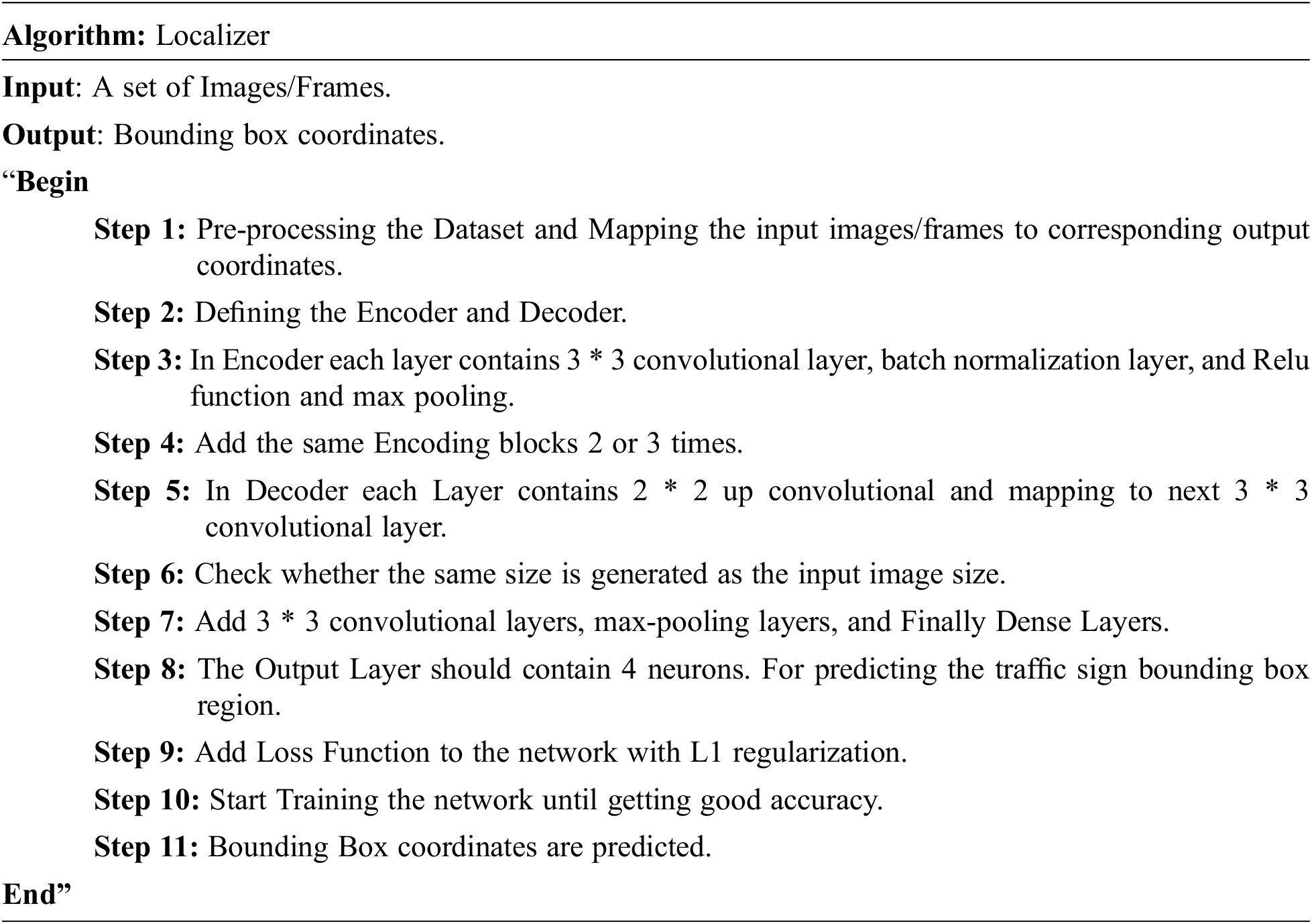
The localizer is implemented by Encoder-Decoder Architecture shown in Fig. 3, SegNet and U-Net [13] inspired a Fully Convolutional Neural Network architecture. The network is made up of two stages: a down sampling encoder and an up - sampling decoder, which are linked together like a residual learning technique [14].

Figure 3: Localizer module diagram
• During down sampling, every convolution blocks in the encoder stage had two 3 * 3 convolution operation, a batch normalization level, a ReLU activation layer, and a 2 * 2 pooling process [15].
• The maximal element’s index is kept for use in up sampling [16]. Each down sampling step doubles the number of characteristic channels [17].
• The map is unsampled at each phase of decoding using a 22-up convolution [18].
• An item is copied to the position stored from the decoder’s appropriate max-pooling layer during up sampling [19].
• The set of feature maps is reduced by half using this up convolution, which is subsequently concatenated with the decoder’s matching feature map [20].
• After that, the feature map is concatenated and processed via two 3 * 3 convolution operation and a ReLU activation layer [21].
• A 11-convolution layer is utilized in the final layer to transfer each element feature representation from the preceding layer to two classes [22].
The Localizer was designed to mirror the SegNet and U-Net designs, resulting in improved identification of tiny indications [23]. During training, U-Net was shown to be resistant to low-resolution image characteristics [24]. In the generally greater comparable layers, there are a considerable number of distinctive channels that allow the user to transfer environment information to various complicated structure [25]. This is a very useful tool for solution to a specific problem in loud circumstances whenever the highly targeted items may not be visible. In the decoder step, SegNet uses an elegant approach of upsampling. Upsampling is performed by the decoders using the max-pooling indices obtained from their respective encoders [26]. This allows the network to separate pixels far more precisely than standard up convolution. To forecast the border boxes, a CNN is incorporated to the encoder and decoder. Some few 3 * 3 convolutional layers, 2 * 2 max-pooling layers, dense layers, and a final layer with four neurons are used in the CNN [27,28].
Eq. (1) is used for calculating the distance between the coordinates predicted by the Localizer Module. MSE Loss function helps the Localizer network to improve the accuracy.
2.2.3 Boundary Extraction Module
The Boundary Extraction Module is shown in Fig. 4, first converting the localizer predicted coordinates into full valued numbers. The traffic sign detection in image patches of size 800X1360 is valued from the bottom right of the input image. The coordinates of the detected region are calculated. A new 32X32X3 square image is resized from the detected boundaries [29].
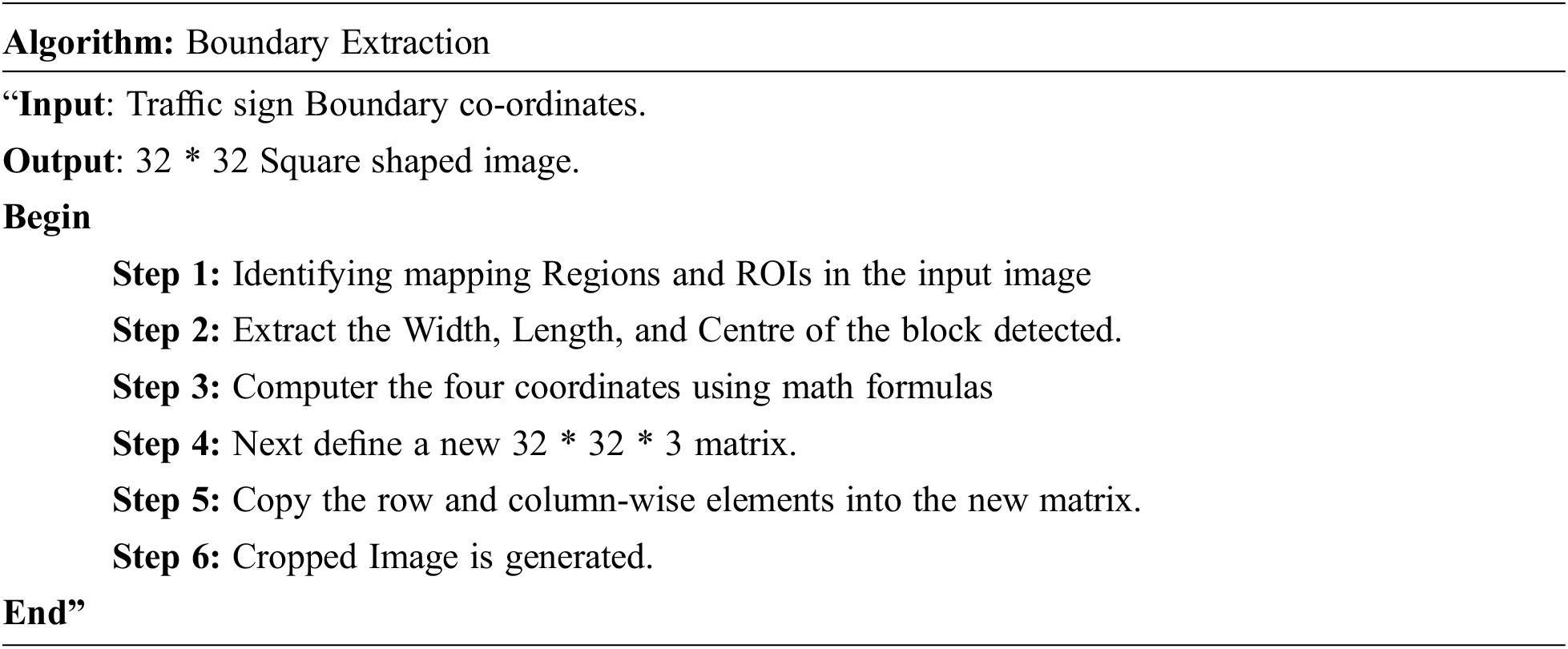
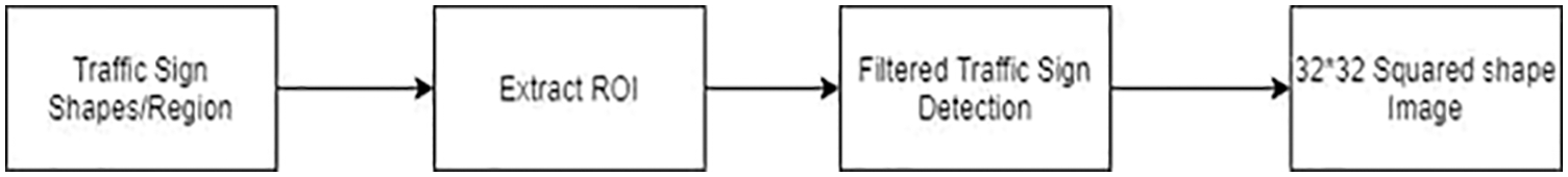
Figure 4: Boundary extractor module diagram
The Classifier Module, as shown in Fig. 5, has a similar architecture to VGG-16. Convolutional blocks are the general definition of the VGG-16 architecture. Two convolutional layer is represented by a Max-pooling in each convolutional block. Three to four times the convolutional blocks were repeated. The next few Fully connected Dense Layers are attached to these convolutional blocks. Finally, the Output Layer contains Softmax as an activation function. ReLu is the activation function for all other levels except the Output Layers. Three convolutional blocks with nine layers, three fully linked layers, and one output layer make up the conventional design. So total of 13 Layers are added to the classifier Module. Since more layers are used for a very small input image. The Neural Network Accuracy must be very good. The Classifier Module defined with 13 layers does a pretty good job, due to the Deep structure for 32*32 Input Image. There are many chances for overfitting the Classifier Neural Network. The Neural Network is modified by adding a few additional layers to reduce overfitting also to increase Accuracy, Precision, and Recall [30].
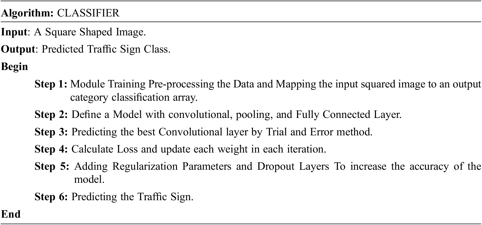
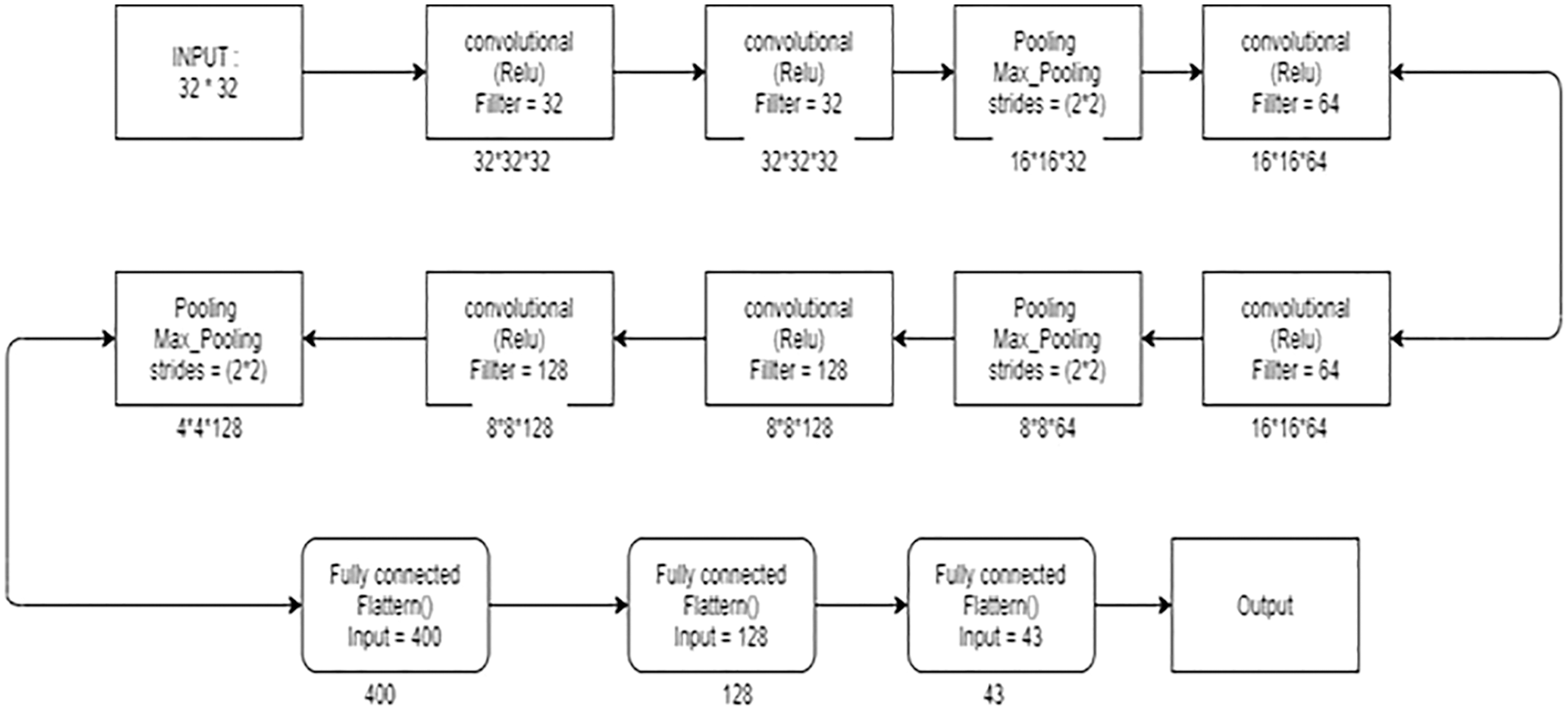
Figure 5: Classifier module diagram
For multi-class classification, the category Cross Entropy Loss method is applied. For each image, we’ll train a CNN to generate a probability over particular classifications. If true labels are one-hot encoded, Categorical Cross Entropy (CCE) is employed.
Eq. (2) is used for calculating the loss between true labels predicted and actual labels. CCE Loss function helps the classifier network to improve the accuracy. The Localizer Module Contains Encoder Blocks which Down samples the Input Image. The input dimensions are 800 * 1360 pixels. The Encoder Block 1 Down samples the Network to 400*680 pixels. The Encoder Block 2 again Down Samples the Network to 200*380 pixels. The Encoder block contains a 3*3 convolutional layer followed by a 2*2 max-pooling layer. The next 2 Decoding blocks are used to Upsample the images. Decoder Block concatenates two encoder blocks that are associated with different filters. The Decoder block also contains Dropout layers to avoid overfitting.
Fig. 6 describes the Encoder and Decoder Blocks in Localizer Module. Next Fig. 6 describes the Convolutional Neural Network Architecture associated with the Encoder-Decoder Module. The Convolutional Neural Network Architecture contains several 3*3 Convolutional Layers and 2*2 Average Pooling Layers. Finally, 3 dense layers and Output layer are added to the CNN. Fig. 7 gives the conclusion that total trainable parameters are more than 22 million. The Localizer Module Network is a very deep convolutional neural network. The Module is trained in the presence of GPU. Training and testing data are divided as 30% and 70% to carry out this experiment. Fig. 8 represents the sample predicted boundary region by the localizer module. The picture is fed into the Neural Network, which returns the boundary coordinates as its output. The length and width of the input picture are used to standardize the boundary coordinates. Finally, Bounding Boxes regions are drawn upon the image.
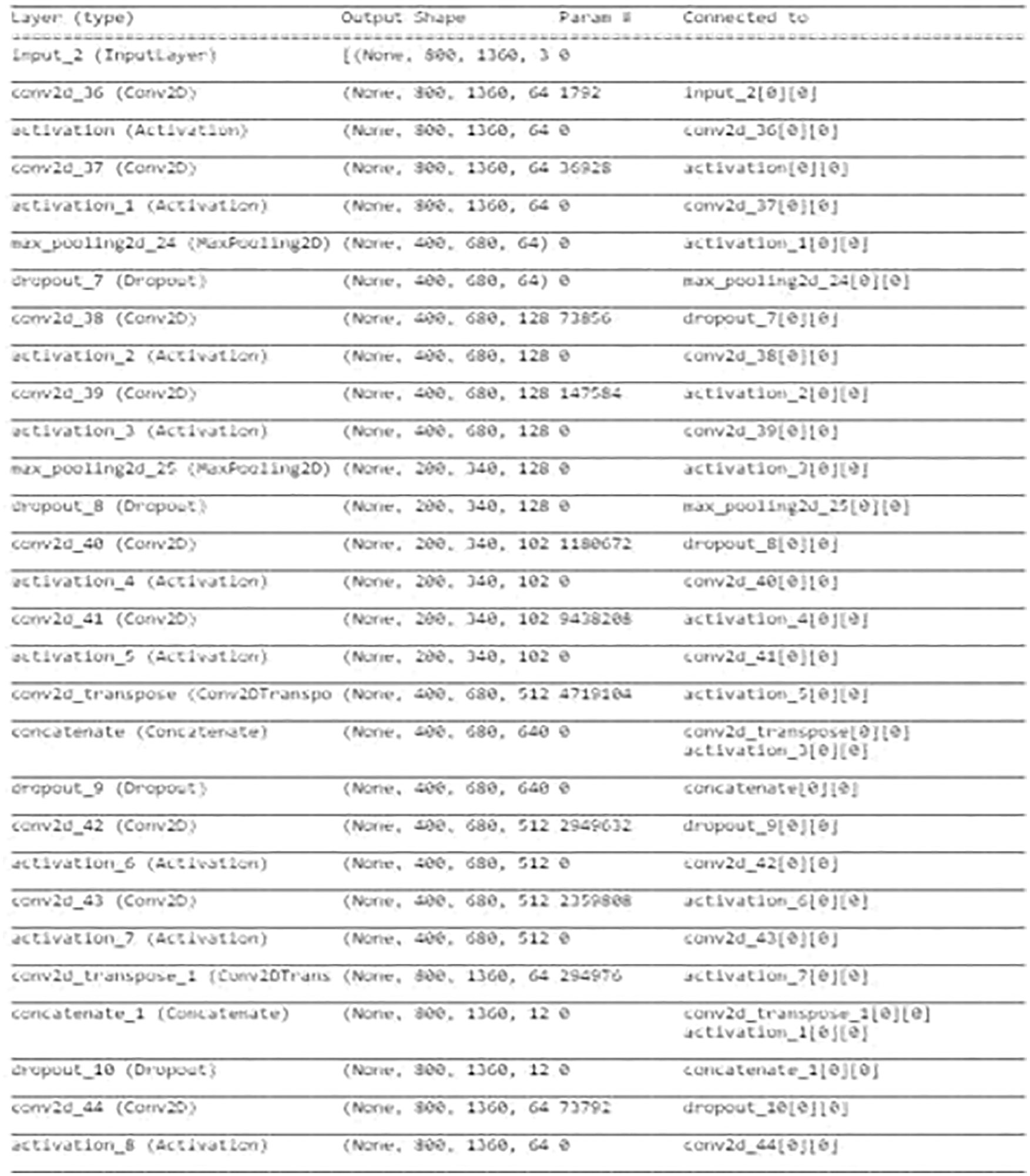
Figure 6: Localizer module encoder-decoder
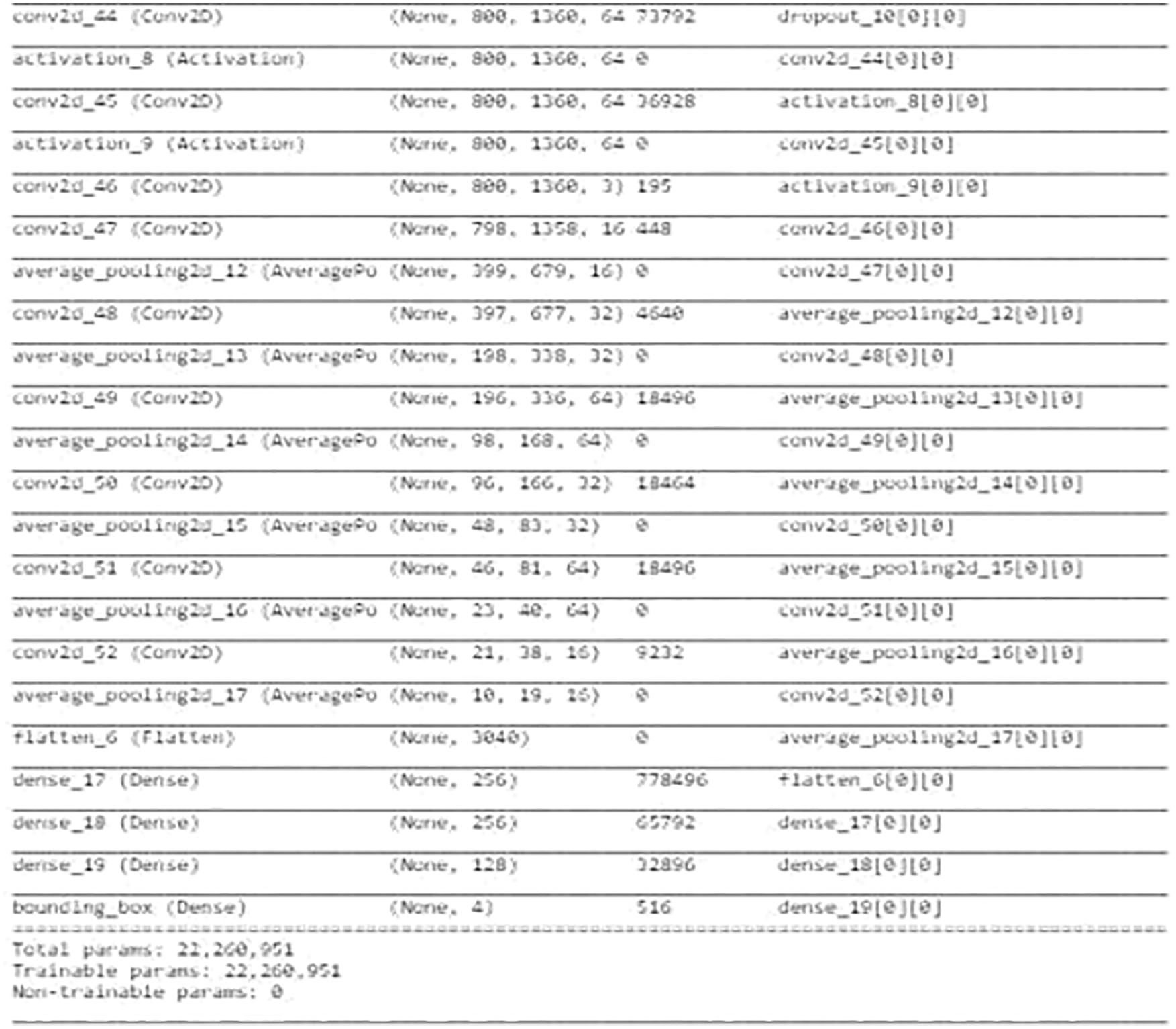
Figure 7: Localizer module neural network
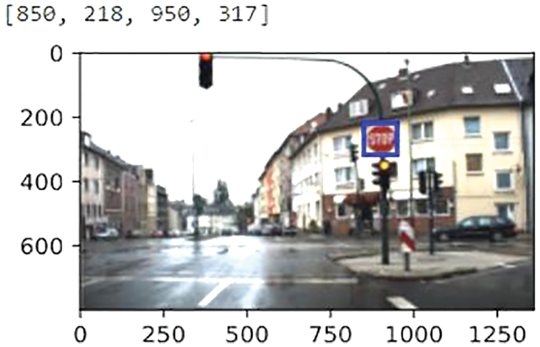
Figure 8: Localizer module sample prediction
The boundary coordinates predicted by the localizer are the corners of the traffic sign in the image. the width, height, and ercenter of the region being computed. After computation, the region is cropped from the road image, and the cropped image is resized into a 32*32 Square image to fit the classifier Neural Network model as shown in Fig. 9.
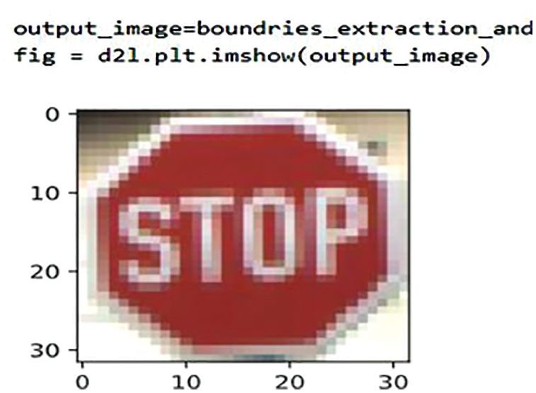
Figure 9: Sample image boundary extraction
The Classifier Module is inspired by the VGG-16 Neural Network. The Classifier Neural Network contains convolutional layers, max-pooling layers, and dense layers. Three different Networks are implemented, they are LeNet Neural Network, VGG Neural Network, and Classifier Neural Network.
LeNet is 7 layers Neural Network. The LeNet contains a convolutional layer, 2*2 Max Pooling layer, and finally 3 dense layers as described in Fig. 10.
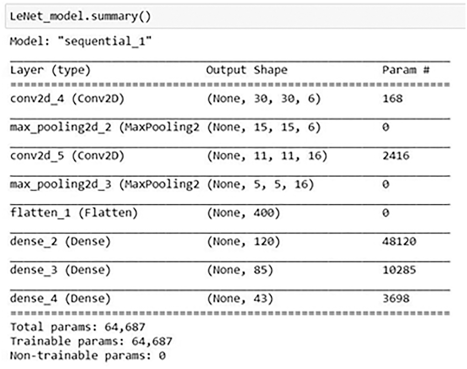
Figure 10: LeNet neural network architecture
The VGG architecture is generally defined as convolutional blocks. Two convolutional layer is represented by a 2*2 Max - pooling in each convolutional block. The convolutional blocks are repeated 3 times. The next 3 Fully connected Dense Layers are attached to these convolutional blocks. Finally, the Output Layer contains Softmax as an activation function as shown in Fig. 11.
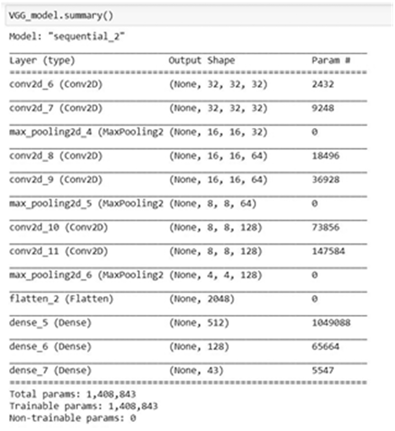
Figure 11: VGG neural network architecture
The Classifier Neural Network contains the same structure as VGG. To overcome the overfitting problem in the VGG Neural Network few layers are added and a few are modified, but the working architecture is almost the same as shown in Fig. 12. The classifier Module Validation Accuracy is 0.9944, Precision Score is 0.9954, Recall Score is 0.9937, and F1- Score is 0.9946
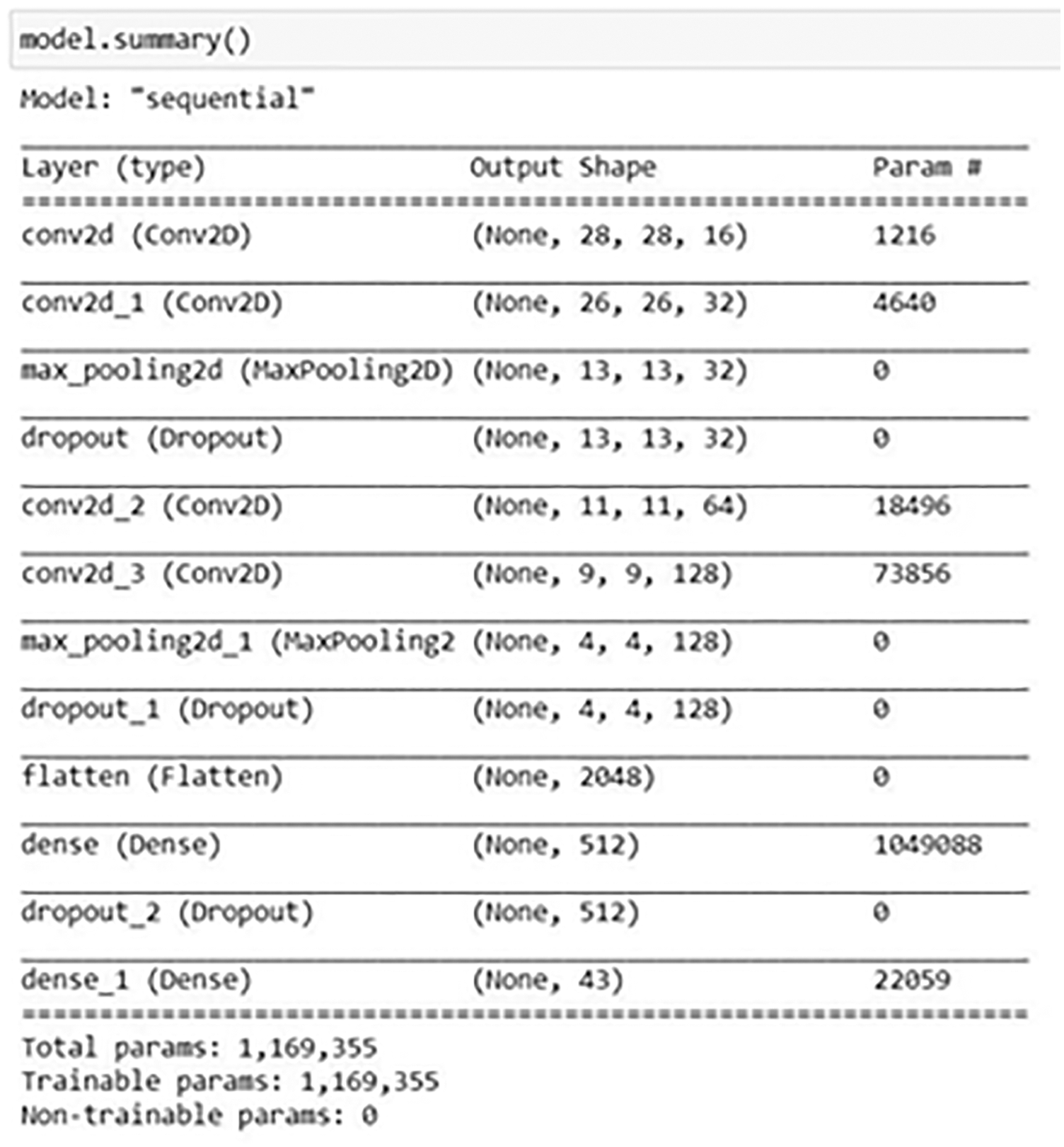
Figure 12: Classifier neural network architecture
We have extracted the real-time road and traffic sign images from the German Traffic Sign Dataset. The Dataset contains nearly 900 images and represents 43 different types of classes. We have labeled all the traffic signs in those images. The labels generated indicate the type of class they belong to and the coordination of the bounding boxes.
The Localizer predicts the traffic sign coordinates in the image. Accuracy and Mean Square Error are the criteria used to assess this module (MSE). The Accuracy for the proposed Module is 0.6805 as shown in Fig. 13. Mean Square Error tells how close the predicted coordinates are to the actual coordinates. MSE is calculated with Eq. (3).
where, MSE – Mean Square error, N – Number of coordinates to be predicted, Ytrue – True coordinate values, and Ypred – Predicated Coordinate Values. The MSE for the proposed Module is 0.3040 obtained based on the execution.
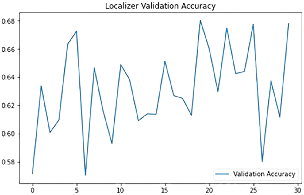
Figure 13: Localizer module validation accuracy
Classifier Neural Network Module classifies the given image to the respective class. So, the evaluation is carried out using the basic parameters used for evaluating predictions namely accuracy, precision, recall, and the f-measure. The Precision for the proposed Module is 0.9954, the Recall for the proposed Module is 0.9937, the Accuracy for the proposed Module is 0.9944 and the F1 Score for the proposed Module is 0.9946. First we do train the dataset with two hidden layer one input and one output layer. In the first iteration we set epoch to some lower value as 10 and its increased gradually until marginal difference was obtained in all the parameters.
The performances of the proposed classifiers are compared with LENET and VGG classifier with the performance metrics of accuracy, precision, recall, and F1 score. The performance of the proposed system outperforms all the other classifiers used in the existing systems. Based on the execution, it is found that the proposed model produced 99.44% of accuracy and 99.54% of precision as shown in Tab. 1.

Figs. 14 and 15 compare the suggested classifiers’ performance to that of other existing classifiers The performance of the proposed Deep Neural Network method is compared with the performance metrics of accuracy and F1 score. Because the suggested technique pre processes the picture using colour space and segmentation with the image threshold, labels the image, and identifies the border coordinates of the traffic sign Region, it outperforms other current methods. The Existing systems are FCNN which are developed with having large hyperparameters, our model uses 1*1 convolution layers and more filters, to reduce the computation power and also reduce the overfitting problem. Deep convolution layers have been added to the classifier neural network which detects edge detection in images. The edge detection system is built with the reference of VGG Neural network. For our model the accuracy is 99.44% when we set the epoch is 17.5 and the Recall is 99.37 when the epoch is 17.5 and its proved that our model produced better results than other algorithms. But do we need to stop here? Yes, because we almost close to 100% of the accuracy, even that can be tested by increasing the epoch.
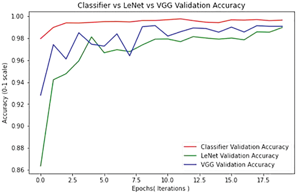
Figure 14: Classifier comparison recall metrics
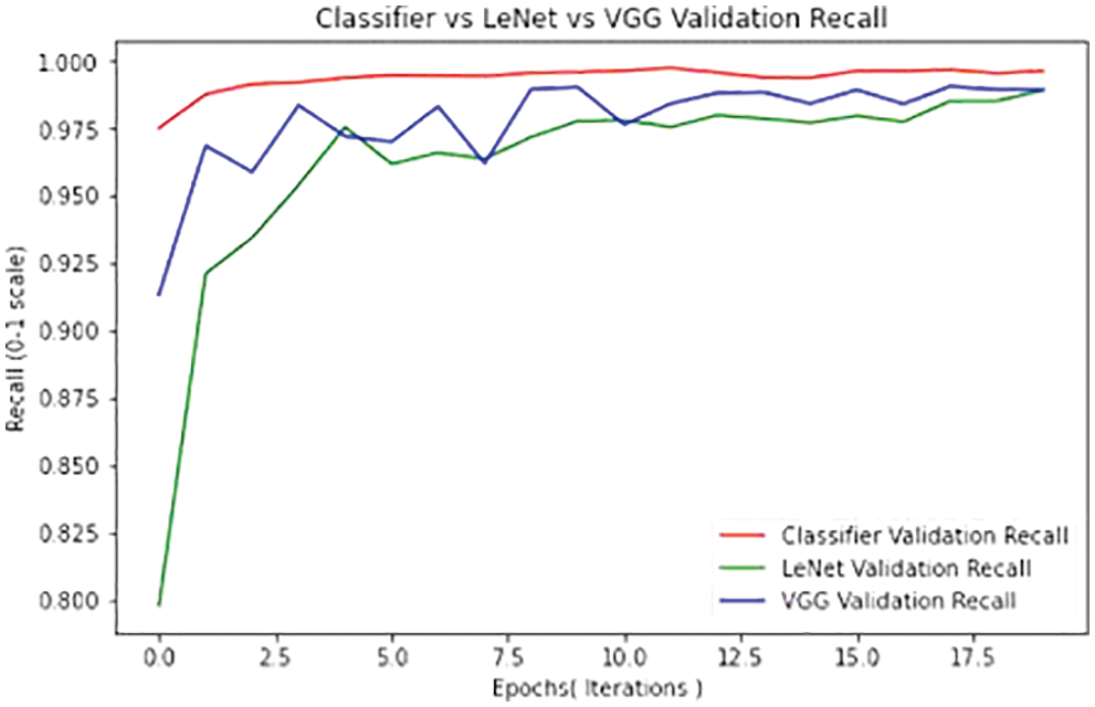
Figure 15: Classifier comparison accuracy metrics
The classifier module’s accuracy is greater, as can be observed. After the recovered signs are cropped off from the image, the Classifier Module does a good job of identifying various types of traffic signs, as seen in the following findings. When the collected indicators from looking at photographs are cropped wrongly, our method fails to produce good results. The Localizer Module ought to be trained with a massive dataset and image Labelling ought to be improved to provide higher Results. The Neural Network can be further trained with different real-time challenging conditions like snow and rain. The Growth in distributive training can be used to train large datasets like CURE-TSD Dataset to improve the Network. Also, the proposed Deep Neural Network method proved that its classifier accuracy, precision, Recall, F1- Score is far better than the other existing methods. To conclude on an considering all the parameters individually its witnessed that approximately 3% performance improvement than compared to LENET and approximately 2% improvement than compared to VGG algorithm.
Funding Statement: The authors received no specific funding for this study.
Conflicts of Interest: The authors declare that they have no conflicts of interest to report regarding the present study.
1. A. Madani and R. Yusof, “Malaysian traffic sign dataset for traffic sign detection and recognition systems,” Journal of Telecommunication Electronic and Computer Engineering, vol. 8, no. 11, pp. 137–143, 2014. [Google Scholar]
2. I. Aljarrah and D. Mohammad, “Video content analysis using convolutional neural networks,” in Proc. 9th Int. Conf. on Information and Communication Systems (ICICS 2018), Irbid, Jordan, pp. 122–126, 2018. [Google Scholar]
3. B. Claus, Y. Zhu, V. Ramesh, M. Pellkofer and T. Koehler, “A system for traffic sign detection, tracking, and recognition using color, shape, and motion information,” in Proc. IEEE: Intelligent Vehicles Symposium, Las Vegas, NV, USA, pp. 255–260, 2005. [Google Scholar]
4. B. Alberto, P. Cerri, P. Medici, P. P. Porta and G. Ghisio, “Real time road signs recognition,” in Proc. IEEE: Intelligent Vehicles Symposium, Istanbul, Turkey, pp. 981–986, 2007. [Google Scholar]
5. X. Changzhen, W. Cong, M. Weixin and S. Yanmei, “A traffic sign detection algorithm based on deep convolutional neural network,” in Proc. IEEE Int. Conf. on Signal and Image Processing, Beijing, China, pp. 676–679, 2016. [Google Scholar]
6. Y. T. Chen, Y. C. Chuang, and A. Y. Wu, “Online extreme learning machine design for the application of federated learning,” in Proc. IEEE Int. Conf. on Artificial Intelligence Circuits and Systems, Genova, Italy, 2020, pp. 188–192. [Google Scholar]
7. L. C. Chen, G. Papandreou, I. Kokkinos, K. Murphy and A. L. Yuille, “Semantic Image Segmentation with Deep Convolutional Nets and Fully Connected Crfs,” IEEE Transactions on Pattern Analysis and Machine Intelligence, vol. 40, no. 4, pp. 834–848, 2018. [Google Scholar]
8. D. Cireşan, U. Meier, J. Masci and J. Schmidhuber, “A committee of neural networks for traffic sign classification,” in Proc. Int. Joint Conf. on Neural Networks, San Jose, California, USA, pp. 1918–1921, 2011. [Google Scholar]
9. D. Ciresan, U. Meier, J. Masci and J. Schmidhuber, “Multi-column deep neural network for traffic sign classification,” Neural Networks, vol. 32, pp. 1–6, 2012. [Google Scholar]
10. D. Moming, D. Liu, X. Chen, Y. Tan, J. Ren et al., "Astraea: Self-balancing federated learning for improving classification accuracy of mobile deep learning applications,” in Proc. Int. Conf. on Computer Design, Abu Dhabi, United Arab Emirates, pp. 246–254, 2019. [Google Scholar]
11. E. Ayoub, M. E. Ansari and I. E. Jaafari, “Traffic sign detection and recognition based on random forests,” Applied Soft Computing, vol. 46, pp. 805–815, 2016. [Google Scholar]
12. F. Hasan and E. Davami, “Eigen-based traffic sign recognition,” IET Intelligent Transport Systems, vol. 5, no. 3, pp. 190–196, 2011. [Google Scholar]
13. M. A. G. Garrido, M. Ocana, D. F. Llorca, M. A. Sotelo, E. Arroyo et al., “Robust traffic signs detection by means of vision and V2I communications,” in Proc. Int. IEEE Conf. on Intelligent Transportation Systems, Washington, DC, USA, 2011, pp. 1003–1008. [Google Scholar]
14. G. Jack and M. Mirmehdi, “Recognizing text-based traffic signs,” IEEE Transactions on Intelligent Transportation Systems, vol. 16, no. 3, pp. 1360–1369, 2014. [Google Scholar]
15. K. He, X. Zhang, S. Ren and J. Sun, “Deep residual learning for image recognition,” in Proc. of the IEEE Conf. on Computer Vision and Pattern Recognition, Las Vegas, NV, USA, pp. 770–778, 2016. [Google Scholar]
16. Z. Jianming, M. Huang, X. Jin and X. Li, “A Real-time Chinese traffic sign detection algorithm based on modified YOLOv2,” Algorithms, vol. 10, no. 4, pp. 127–136, 2017. [Google Scholar]
17. U. Kamal, T. I. Tonmoy, S. Das and M. K. Hasan, “Automatic traffic sign detection and recognition using segu-net and a modified tversky loss function with L1-constraint,” IEEE Transactions on Intelligent Transportation Systems, vol. 21, no. 4, pp. 1467–1479, 2020. [Google Scholar]
18. J. M. L. Castellano, I. M. Jimenez, C. F. Pozuelo and J. L. R. Alvarez, “Traffic sign segmentation and classification using statistical learning methods,” Neurocomputing, vol. 153, pp. 286–299, 2015. [Google Scholar]
19. M. Andreas, M. M. Trivedi, B. Thomas and B. Moeslund, “Vision-based traffic sign detection and analysis for intelligent driver assistance systems: Perspectives and survey,” IEEE Transactions on Intelligent Transportation Systems, vol. 13, no. 4, pp. 1484–1497, 2012. [Google Scholar]
20. S. Ying, P. Ge and D. Liu, “Traffic sign detection and recognition based on convolutional neural network,” in Proc. Chinese Automation Congress, Hangzhou, China, 2019, pp. 2851–2854. [Google Scholar]
21. S. Christian, W. Liu, Y. Jia, P. Sermanet, S. Reed et al., “Going deeper with convolutions,” in Proc. of the IEEE Conf. on Computer Vision and Pattern Recognition, Boston, MA, USA, pp. 1–9, 2015. [Google Scholar]
22. T. Domen, and D. Skocaj, “Deep learning for large-scale traffic-sign detection and recognition,” IEEE Transactions on Intelligent Transportation Systems, vol. 21, no. 4, pp. 1427–1440, 2019. [Google Scholar]
23. D. Temel, M. H. Chen and G. AlRegib, “Traffic sign detection under challenging conditions: A deeper look into performance variations and spectral characteristics,” IEEE Transactions on Intelligent Transportation Systems, vol. 21, no. 9, pp. 3663–3673, 2019. [Google Scholar]
24. R. Timofte, K. Zimmermann and L. V. Gool, “Multi-view traffic sign detection, recognition, and 3D localization,” Machine Vision and Applications, vol. 25, no. 3, pp. 633–647, 2014. [Google Scholar]
25. Y. Yi and F. Wu, “Real-time traffic sign detection via color probability model and integral channel features,” in Proc. Chinese Conf. on Pattern Recognition, Changsha, China, pp. 545–554, 2014. [Google Scholar]
26. Y. Yang, H. Luo, H. Xu and F. Wu, “Towards real-time traffic sign detection and classification, ” IEEE Transactions on Intelligent Transportation Systems, vol. 17, no. 7, pp. 2022–2031, 2015. [Google Scholar]
27. Z. Fatin and B. Stanciulescu, “Real-time traffic-sign recognition using tree classifiers,” IEEE Transactions on Intelligent Transportation Systems, vol. 13, no. 4, pp. 1507–1514, 2012. [Google Scholar]
28. Z. Fatin, and B. Stanciulescu, “Real-time traffic sign recognition in three stages,” Robotics and Autonomous Systems, vol. 62, no. 1, pp. 16–24, 2014. [Google Scholar]
29. X. R. Zhang, W. F. Zhang, W. Sun, X. M. Sun and S. K. Jha, “A robust 3-D medical watermarking based on wavelet transform for data protection,” Computer Systems Science & Engineering, vol. 41, no. 3, pp. 1043–1056, 2022. [Google Scholar]
30. X. R. Zhang, X. Sun, X. M. Sun, W. Sun and S. K. Jha, “Robust reversible audio watermarking scheme for telemedicine and privacy protection,” Computers, Materials & Continua, vol. 71, no. 2, pp. 3035–3050, 2022. [Google Scholar]
 | This work is licensed under a Creative Commons Attribution 4.0 International License, which permits unrestricted use, distribution, and reproduction in any medium, provided the original work is properly cited. |