DOI:10.32604/iasc.2023.028944
| Intelligent Automation & Soft Computing DOI:10.32604/iasc.2023.028944 | |
| Article |
Robust ACO-Based Landmark Matching and Maxillofacial Anomalies Classification
1LTSIRS LR20ES06, Institut National des Sciences Appliquées et de Technologie INSAT, Université de Carthage, Tunisia
2Department of Information Technology, College of Computer and Information Sciences, Princess Nourah bint Abdulrahman University, P.O. Box 84428, Riyadh 11671, Saudi Arabia
*Corresponding Author: Hela Elmannai. Email: hselmannai@pnu.edu.sa
Received: 22 February 2022; Accepted: 21 April 2022
Abstract: Imagery assessment is an efficient method for detecting craniofacial anomalies. A cephalometric landmark matching approach may help in orthodontic diagnosis, craniofacial growth assessment and treatment planning. Automatic landmark matching and anomalies detection helps face the manual labelling limitations and optimize preoperative planning of maxillofacial surgery. The aim of this study was to develop an accurate Cephalometric Landmark Matching method as well as an automatic system for anatomical anomalies classification. First, the Active Appearance Model (AAM) was used for the matching process. This process was achieved by the Ant Colony Optimization (ACO) algorithm enriched with proximity information. Then, the maxillofacial anomalies were classified using the Support Vector Machine (SVM). The experiments were conducted on X-ray cephalograms of 400 patients where the ground truth was produced by two experts. The frameworks achieved a landmark matching error (LE) of 0.50 ± 1.04 and a successful landmark matching of 89.47% in the 2 mm and 3 mm range and of 100% in the 4 mm range. The classification of anomalies achieved an accuracy of 98.75%. Compared to previous work, the proposed approach is simpler and has a comparable range of acceptable matching cost and anomaly classification. Results have also shown that it outperformed the K-nearest neighbors (KNN) classifier.
Keywords: Maxillofacial anomalies; cephalometric landmarks similarity; chi-square distance; quadratic assignment problem; ant colony optimization; SVM
When confronted with a wide range of clinical manifestations and pathological symptoms, practitioners have to conduct a thorough clinical examination to determine the cause of the dysfunction, functional disorders (such as swallowing, chewing, breathing, and phonation), social acceptance issues, and pain [1]. These are all symptoms of cranial-maxillofacial anomalies [2]. Medical imagery was developed to improve surgeons' performance by providing new compliant and absolute tools that could be integrated into the diagnosis, planning, and simulation, and which outcomes could serve for surgery optimization.
Preoperative preparation, which may require long hours, is a crucial step in maxillofacial surgery. Furthermore, the outcome of the cephalometric landmark matching [3] will determine both the functional and aesthetic results. Obviously, an accurate identification of any maxillofacial anomalies is required for oral and maxillofacial surgeries as well as orthodontic treatments. The most commonly used image modalities for this purpose are two-dimensional (2D) X-rays of the human head. High resolution, well-defined measurements are now possible thanks to modern cephalometry. Because manual annotation of cephalograms is time-consuming and potentially inaccurate, there is an urgent need for a computerized tool that can extract and measure diagnostically-relevant properties of the skull and allow for automated detection and classification of maxillofacial anomalies. To address the issue of the preoperative preparation problem, we have developed a framework to automate the matching of cephalometric landmarks and optimize preoperative planning of the maxillofacial surgery. The objectives of this research was to provide an efficient support to the preoperative planning of maxillofacial surgery by means of:
– developing a framework to automate the matching between cephalometric landmarks
– providing an automatic abnormality classification.
The remainder of this article is structured as follows: Section 2 provided a review of similar works. Section 3 introduced the dataset attributes, as well as the locations and labels of landmarks. Section 4 described the proposed approach. The experiment design and related results and evaluation were provided and discussed in Section 5. Section 6 summarized the key features of the proposed work and suggested some potential perspectives.
The cephalometric analysis is basically used for orthodontic diagnosis [4–6]. Landmarks determined on a Skeletal X-ray images are needed for this analysis as they provide the required measurements and distances for the diagnosis and treatment. However, such an analysis could be time-consuming, inaccurate and dependable on the experiment considerations. Besides, landmarks identification is subject to the inter-observation variability [7]. Thus, a computer aided detection could provide objectivity and efficiency for landmark as well as anomaly detection, recognition and classification. In this context, it is worth reviewing the rich literature with the various studies that have addressed the cephalometric landmark analysis.
In [8], an automatic analysis of lateral cephalograms for malformation classification and assessment of dental growth using the tree regression voting method is proposed. The achieved Success Detection Rate (SDR) was 73.37%, 84.46% and 90.67% for respectively 2 mm, 3 mm and 4 mm ranges. The mean landmark error was 1.69 ± 1.43 mm. Although the proposed algorithm provided comparable results to the manual marking, the performance depends on the training set and the model consistency is limited by the variety of the training set. In [9], the authors propose a Fully Automatic Landmark Annotation System (FALA) for the search for cephalometric landmarks in lateral cephalograms. Their purpose is to perform a classification of skeletal malformations based on the Random Forest regression-voting in order to detect the position, scale and orientation of the skull and then locate the landmarks by a Constrained Local Model framework. The experiments show that the method’s efficiency depends on the patch size and training and reached a detection rate SDR of 84.70%, 92.62% and 96.30% for respectively 2 mm, 3 mm and 4 mm ranges. The obtained mean landmark error was 1.20 ± 0.06 mm. Although the FALA system provided more accurate results than the manual annotations, the system depends on the quality of the training set.
A great deal of research has taken advantage of the flourishing deep learning technique in anomalies and diseases detection [8–11]. In 2017, Arik et al. [12] use a convolutional neural network for a binary classification and achieved success detection rates of 75.58%, 75.37%, and 67.68% at a 2 mm range for three different datasets, respectively. The achieved overall accuracies for pathology classification, for two test sets were of 75.92% and 76.75%. The approach has lower performance compared to previous works and is limited by the dissimilarity of the training and test images. Relying on a new architecture, the authors in [13] succeed to achieve the state-of-the art results and reached a nearly 6% higher accuracy than the previous approaches. Similar to supervised learning based approaches, the system performance remains dependent on the training set size and content. Song et al., introduce an automatic quantitative cephalometry for orthodontics using a deep convolutional neural network (DCNN) [14]. The obtained SDR was 1.84 ± 1.79 m while the successful detection rate was 71.7% within a 2 mm range. Unfortunately, the suggested method reached unsatisfactory results when processing cases with huge anatomy differences and the predicted results are not similar to the ground-truth.
In this work, we used the public X-ray dataset proposed at the International Symposium on Biomedical Imaging on cephalometry landmark detection challenge ISBI2015 [15] and ISBI2019 [13]. The X-Ray images are lateral cephalograms acquired from 400 patients including 235 females and 165 males. The sample ranged between 7–76 years in age with a mean age of 27 years. Each image contains 19 landmarks manually marked by two clinical orthodontists as shown in Fig. 1. The landmarks were chosen based on the common structures used in cephalometric evaluations such as Wits Appraisal. The training set consists of 150 images while Test1 and Test2 datasets are made up of 150 and 100 images, respectively, in TIFF format. The image resolution is 1935 × 2400 pixels and the spatial resolution is about 0.1 mm.
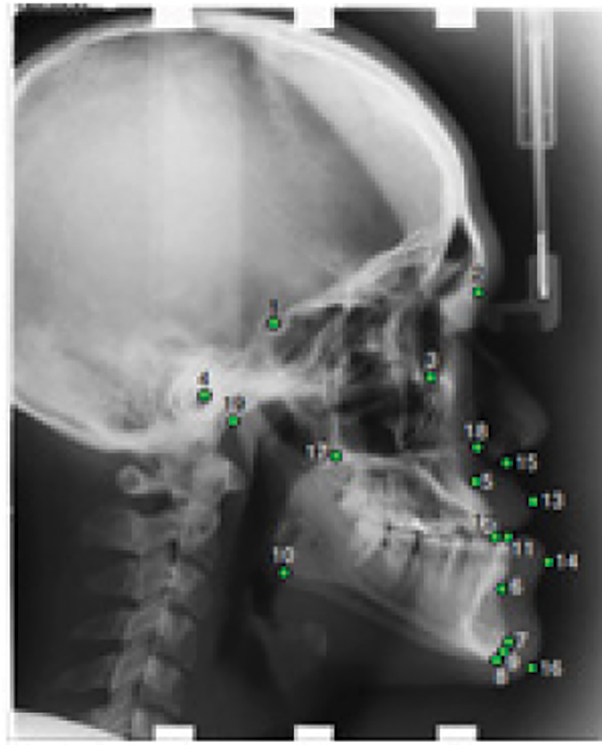
Figure 1: Cephalogram annotation showing the 19 landmarks
Several state-of-the-art methods were proposed and verified on this dataset despite its relatively small benchmark size. The highest results were achieved by Lindner et al., [9] using the random-forest and achieving a detection rate of 74.84% at a 2 mm precision range. The precision range is the error range accepted between landmark position and manual annotation. Ibragimov et al., used a Haar-like [15] feature extraction then a random-forest regression and a global-context shape refinement. Later, in 2017, the authors used a CNN for a binary classification and improved the results to reach a 75.3% prediction accuracy within the same range [16]. Qian et al., improved the Faster R-CNN [17] and proposed a dedicated deep architecture called the CephaNet in [13]. The obtained accuracy results using this approach are 82.5% and 72.4% on Test1 and Test2 datasets, respectively, at a 2 mm range; this means a 6% higher improvement than any of the other conventional methods.
Cephalometry is a concept that was first introduced by Broadbent and Hofrath in 1931 [18]. It is a measurement of the dimensions of the pinnacle between the bone and soft tissue landmarks, used to predict the craniofacial growth, set up a treatment, and check various cases.
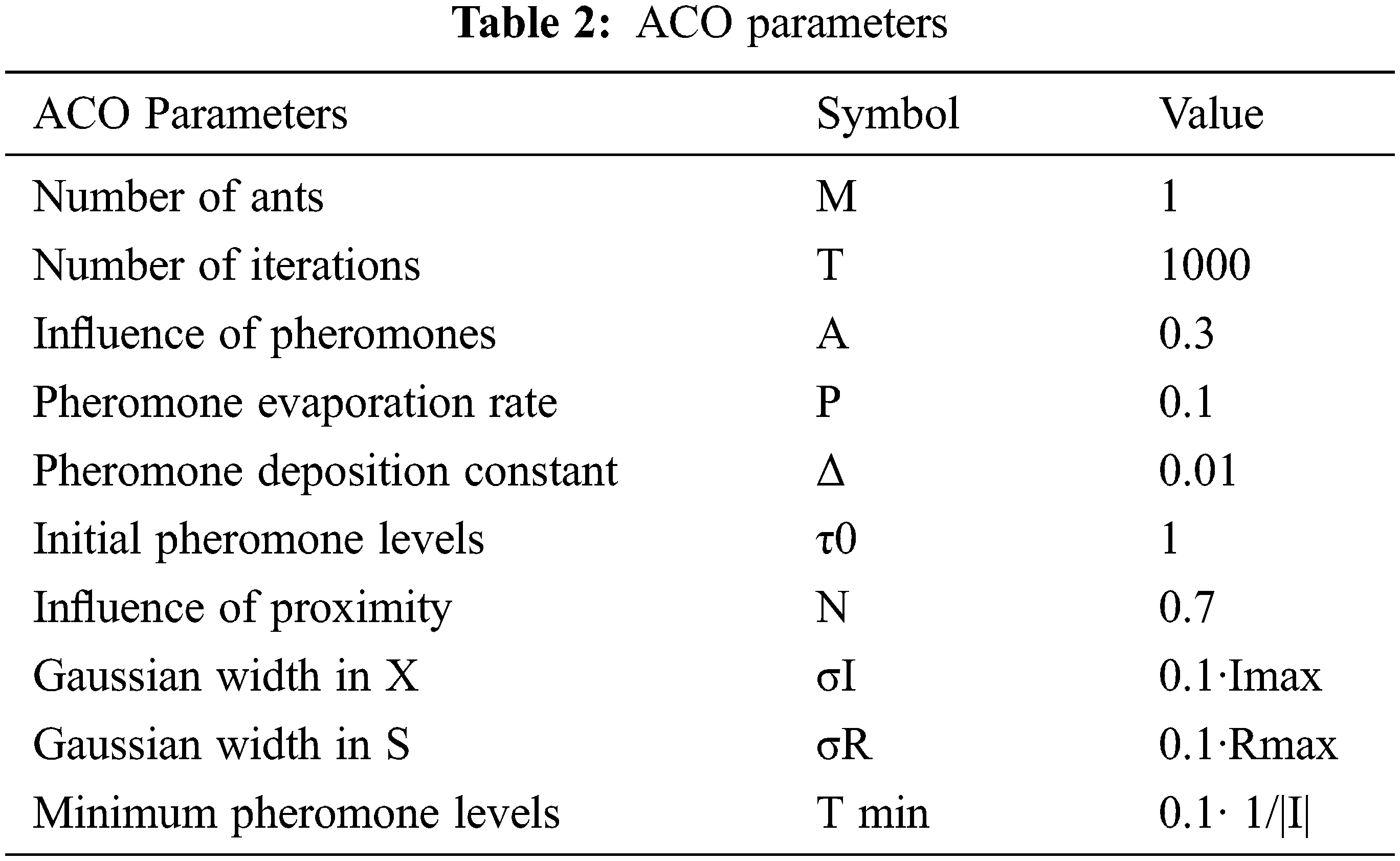
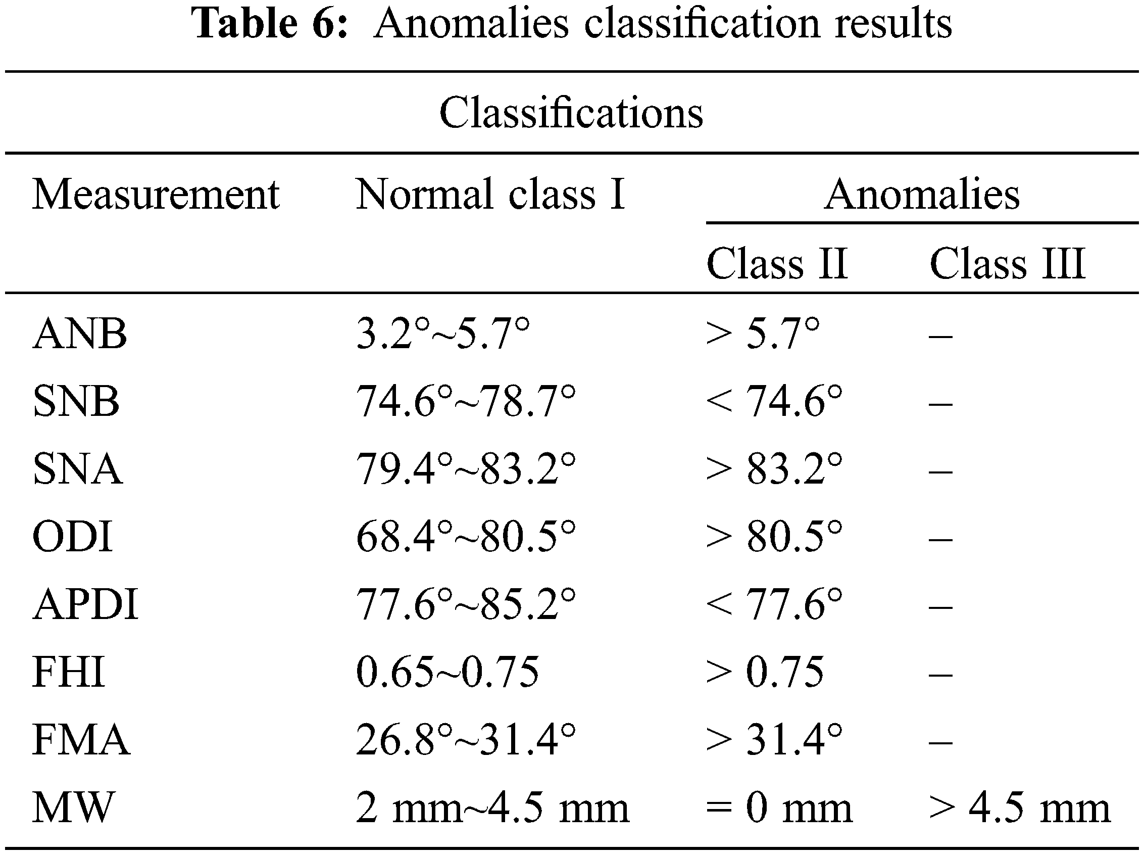
The conventional methodology for landmarks localization depends on a manual tracing of the radiographic images. Such a manual tracing which determines the anatomical landmarks on X-ray images is a time-consuming process and might be fallible even when achieved by an experienced physician. Consequently, several researchers have focused on automating the landmark detection process [19,20]. Regarding the bottom truth information for analysis, landmarks are initially marked manually and reviewed by two experienced medical experts. Eight anatomical angles measurements are defined using the 19 landmarks [15]. Tab. 1 summarizes the parameters used in this work.

Establishing the landmark matching allows the analysis of the anatomical structures by detecting the deformation between the landmarks of the model and those of the test. Here, we introduced the problem of point matching and correspondence and proposed an ACO-based algorithm to determine the matching by incorporating the proximity information. We would prove that the consideration of proximity seemed rather advantageous in points matching. Afterwards, we adopted a support vector machine (SVM) to classify and predict the maxillofacial anomalies relying on a comparison with the k-nearest neighbor (KNN) method. To prove the feasibility and effectiveness of our ACO- and SVM-based approach, we conducted several experiments on normal and abnormal cases.
This research aimed to assist the maxillofacial surgery in automating and optimizing the preoperative planning of maxillofacial procedures by implementing an automatic correspondence approach of the 2D structures of the facial mass and, therefore, the recognition of anomalies. The general framework is drawn in the below Fig. 2.
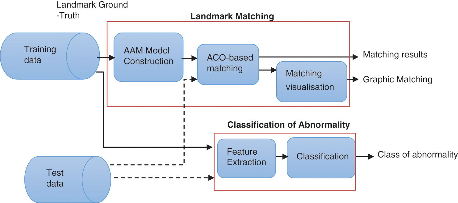
Figure 2: Detailed methodology
This approach consists of two main procedures:
1. First, we proposed a new method based on the Active Appearance Shape (AAM) algorithm to extract the cephalometric point model. The Shape Context was used to induce a singular descriptor (feature vector) for each point of an object contour or surface. This descriptor was employed jointly with a b-spline free-form deformation grid, for the full creation of point mappings between surfaces of patient datasets.
In this context, we proposed an ACO based approach to obtain an accurate matching between interest landmarks of models and test landmarks using the Chi-square distance. Furthermore, we used the sigmoid function for anomalies visualization.
2. The classification of anomalies is based on an SVM classification of the maxillo-facial anomalies. The results would then be compared to those achieved with the k-nearest neighbor (KNN) method.
In what follows, we detailed the landmark matching methodology and anomalies classification.
4.1 Landmark Matching Methodology
The Active Appearance Model (AAM) is a deformable statistical model of the shape for a class of deformable objects. This generative model aims to retrieve a parametric description through optimization. The AAM model uses a training set as follows:
• Extraction of the characteristics of all the training images using the characteristics function.
• Distortion of the images based on the characteristics of the reference shape.
• Vectorization of the distorted images.
• Application of the Principal Component Analysis (PCA) on the acquired vectors for dimension reduction.
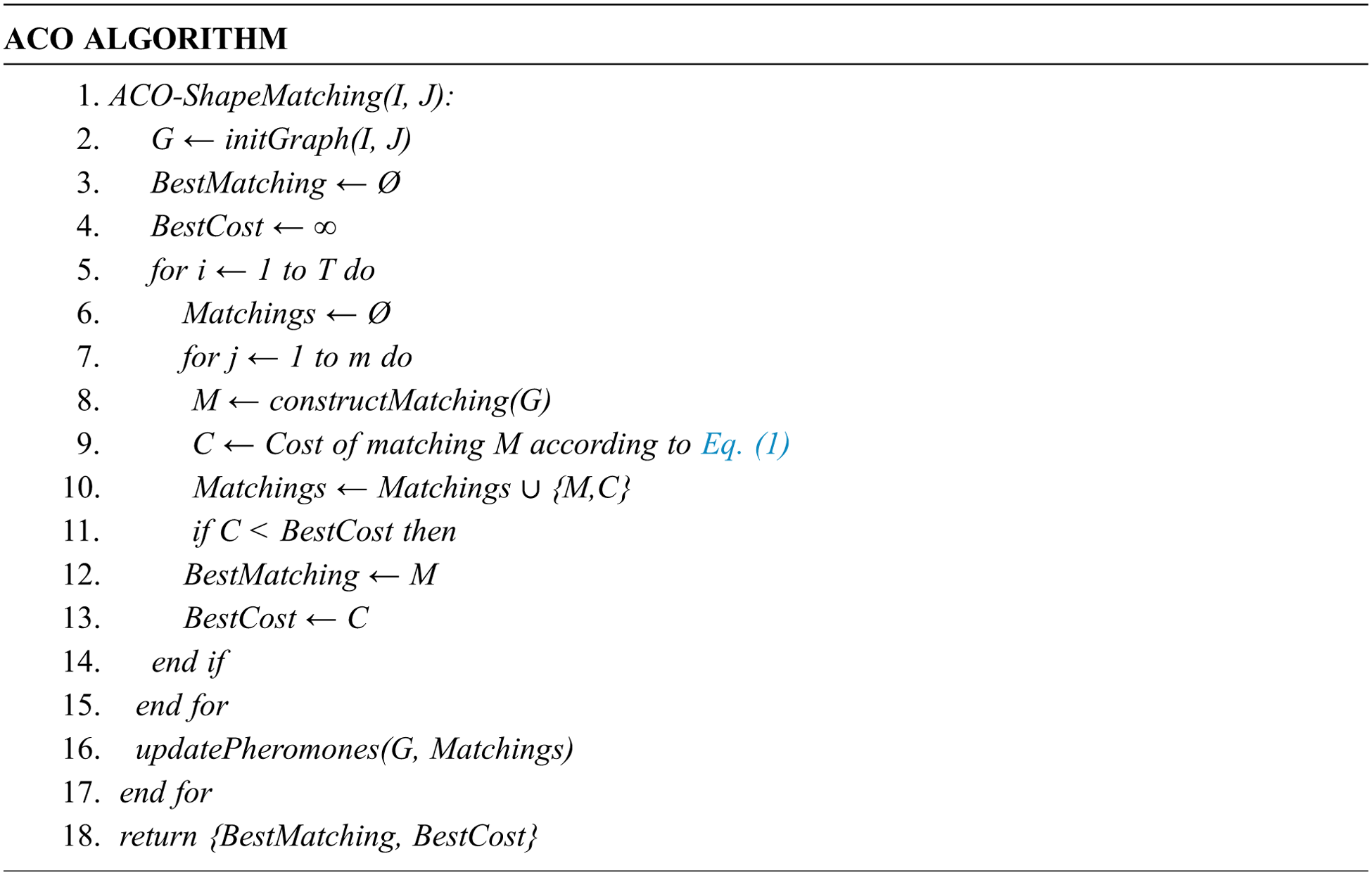
To carry out the matching between the model and test landmarks, we used the ACO optimization algorithm that was detailed in the next paragraph. Our main contribution was to use a metaheuristic approach, which is based on the ACO algorithm to solve the correspondence problem of cephalometric landmarks.
4.1.2 ACO Based Landmark Matching
The cephalometric landmarks correspondence can be modeled as a graph matching problem. In this paper, we proposed to search the optimal matching using the ACO, which is a meta-heuristic approach that has been used to solve many combinatorial optimization problems such as: Vehicle Routing [20,21], Traveling Salesman [22,23], Network Model [24], and Quadratic Assignment (QAP) [16,25,26]. We applied the correspondence points problem theory which integrates proximity information [27–29] and explains how the ACO algorithm is used to determine the landmarks matching.
i) The Quadratic Assignment Concept:
Considering two sets I and J, the graph correspondence problem can be defined as finding the best mapping over the two sets, which minimizes the cost function. π denotes the mapping that verifies that
∀i ∈ I,∃ j ∈ J : π(i) = j. We aimed to find the optimal matching π∗, expressed by (1).
COST is the function that measures the matching π in relation to the shapes determined by the points in the I and J sets. Without loss of generality, we also assume that |I| ≤ |J|. QAP [30] is used to represent this matching. As QAP is an NP-hard problem, we proposed to solve it using a heuristic that imitates the ants’ behavior [31,32]. The adopted concept was to assign a set of facilities to a set of locations [33]. These locations are separated by distances. Assigning the facilities to locations is constrained by minimizing the sum of products between flows and distances [14,34,35].
The optimal correspondence for two contours is computed by our ACO algorithm and displayed in Fig. 3. The obtained ACO mapping between the two red and blue shapes is represented by lines.
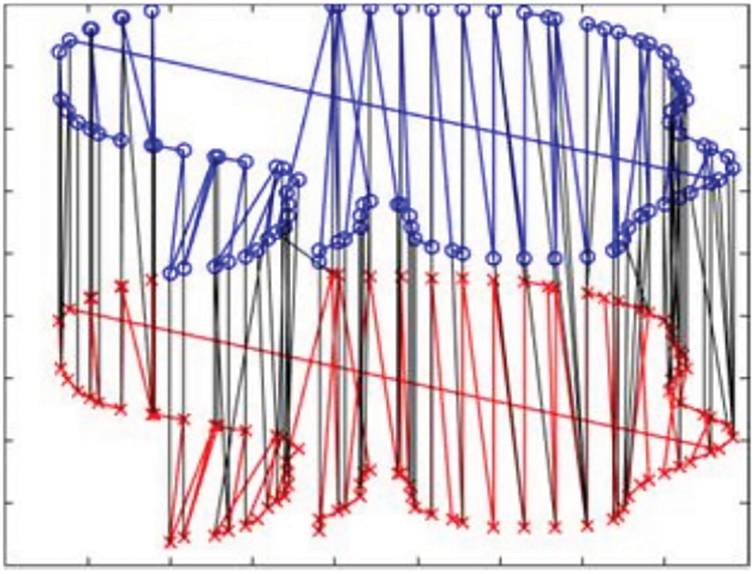
Figure 3: ACO-based Mapping
ii) Proximity Information:
The proximity principle asserts that when two points are close on one shape, their matched points in the second shape should also be close. Considering i from the set I and j from the set J, the mapping for each point in the set I to its mapping in J is presented by π [36,37]. Besides point ordering, we also considered the distances between point pairs on the same shape. By adding proximity information to a shape descriptor R, we obtained the general objective function of QAP as expressed in (2) where v is the weights parameters with 0 ≤ ν ≤ 1. The similarity term
where 0≤
In our case, the shape distances are normalized with respect to contour length and order preservation. As for proximity, which is emphasized more in the local neighborhood, we proceeded with the Gaussian weights. We obtained the Gaussian widths σR and σI for the descriptor distances and proximity. The QAP advantage is its suitability to any contour matching problem regardless of the shape with the sole condition that the distance factor is considered. The ACO is an iterative algorithm, where pheromone is used to reinforce the traversal of the edges providing optimal solutions. Pheromone evaporates during the iterations at an evaporation rate ρ, 0 ≤ ρ ≤ 1 as presented in Fig. 4. Pheromone is updated regularly.
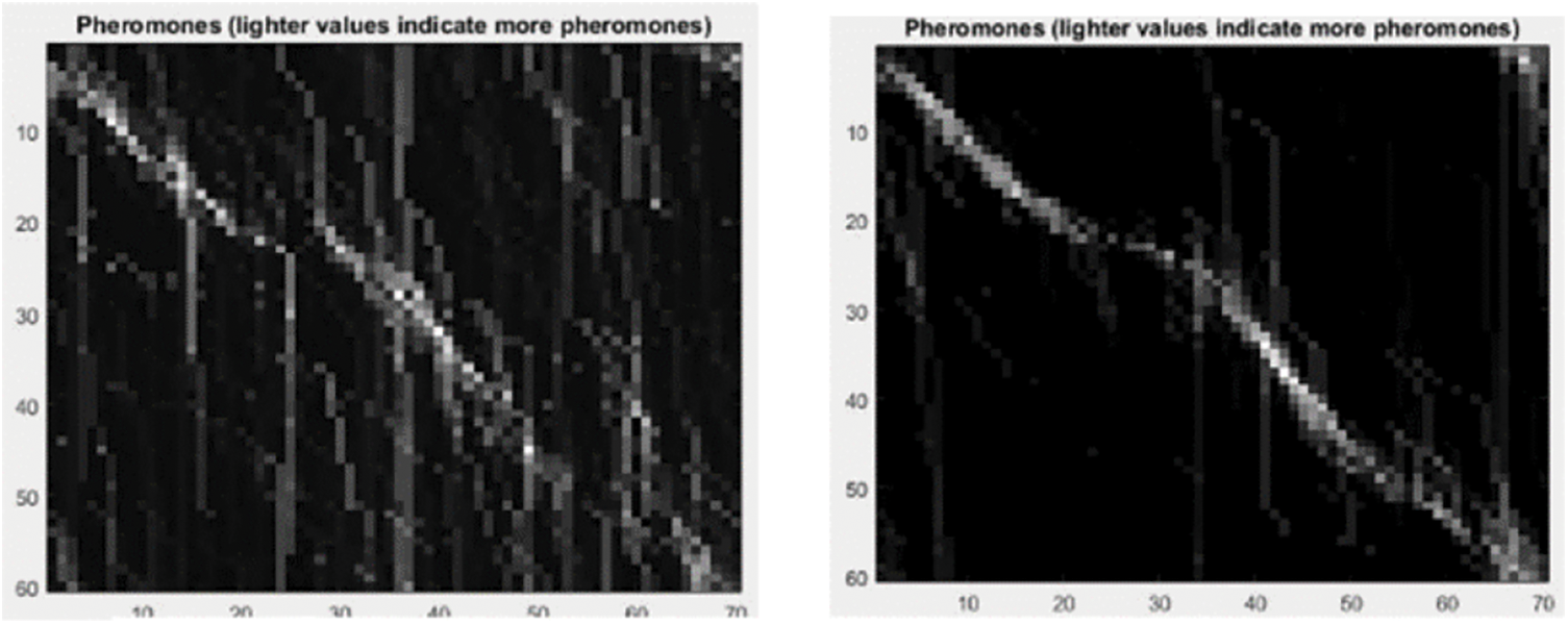
Figure 4: Pheromone deposit for 100 and 1,000 iterations
– Pheromone Evaporation: For all edges (i, j), i.e., vertices connecting two sets of points, new pheromone is deposited only on edges that are traversed by the ants:
– Pheromone constant deposition:
where
iii) ACO Based Approach
Tab. 2 shows the list of parameters used in our ACO-based approach to establish the matching algorithmic rules and the various values selected in the experiments. The auxiliary parameter Imax is set to the maximum proximity in I while Rmax is set to the maximum descriptor distance.
iv) Chi-square Distance
The similarity between points from the two sets I and J was computed by the shapes Chi-square Distance. Considering an nxp frequency matrix (fij), the chi-square distance
For a normalized representation, the sigmoid activation function converts the weighted sum of the diagonal of the matching matrix to a value between 0 and 1. A continuous line means that there is no detected malformation while a discontinuous sigmoid representation indicates the existence of a malformation.
4.2 Maxillofacial Anomalies Classification
Our aim was to classify maxillofacial anomalies based on SVM. The obtained results were compared to those of the k-nearest neighbors (KNN) clustering algorithm. The SVM algorithm is a kernel machine based on a set of kernel functions. Basically, the kernel function maps the data into a higher dimensional space. The kernel Radial Basis function (RBF) is given by (8). The RBF has been widely used for nonlinear problem classification [38,39]. ||.||2 is the squared Euclidean distance, x and x’ are feature vectors. δ is a hyperparameter.
5 Experimental Results and Discussion
In this section, we described and discussed the achieved matching and classification results.
5.1 Cephalometric Landmarks Matching Experiment
In this study, we considered the sum of the distances over the points of the graph pairs, which is a scoring scheme proposed by Karlsson and Ericsson [40]. Our method was compared to the Hungarian algorithm later on. The results show that the ACO algorithm generally provides better matching as it provides the minimal COST. According to Fig. 5, the best obtained cost is 0.23. The displayed results were obtained based on the set of parameters presented in Tab. 3. The ACO was executed for 1000 iterations. The next subsections detailed the matching results for both of normal and malformation cases.
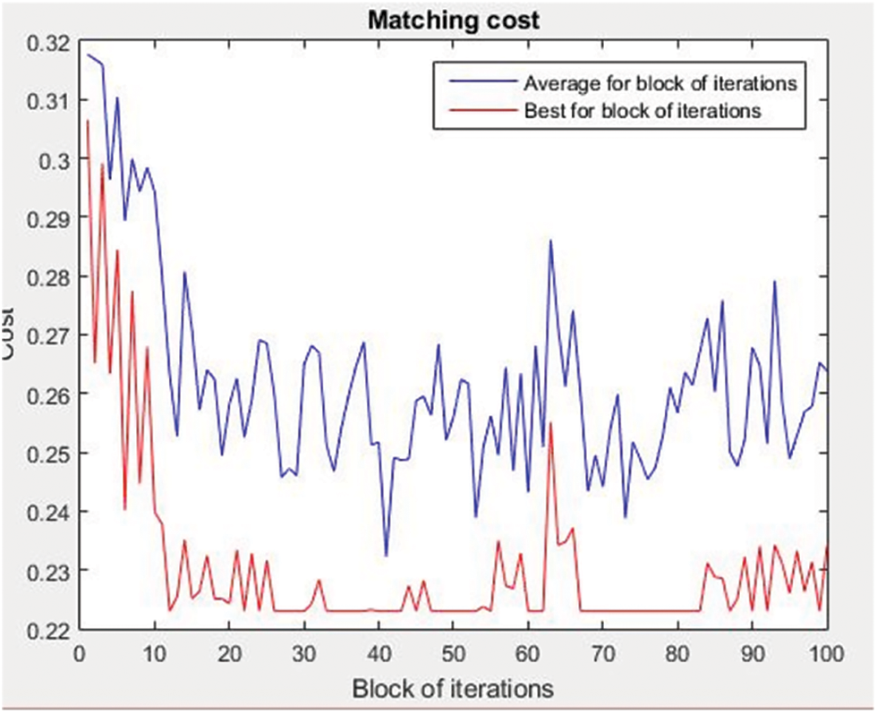
Figure 5: The optimal matching with the ACO algorithm

5.1.1 Results of Malformation-Free Images
In this test, we used malformation-free images containing 19 landmarks. The matching was performed between the cephalometric points of the model landmarks and the test landmarks. Fig. 6 shows the matching based on proximity information and order preservation. The outcome indicates that the matchings tend to be intuitive and yield the best results.
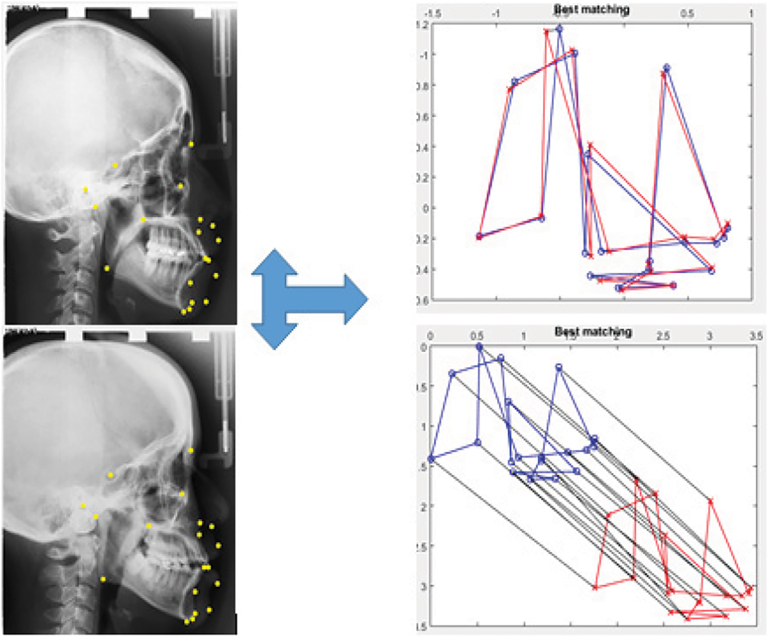
Figure 6: Pheromone deposit during 100 and 1,000 iterations
In this study, we referred to K as a matrix of <19 × 2> dimension containing the matching values as follows: vertex K (i, 1) on shape 1 is matched to vertex K (i, 2) on shape 2. The best obtained matching results for each Landmark model vertex K (i, 1) on shape 1 corresponds to the same Landmark for image test vertex K (i, 2) on shape 2, where i is the landmark index.
5.1.3 Similarity Matrix Between Matching Points
Let S be a 19 × 19 matrix that represents the similarity for the specified descriptor. The similarity values are determined using the chi-square, where S(i,j) is the similarity between the i-th vertex/point of shape 1 and the j-th vertex/point of shape 2, e.g., 0.0769 mm is the distance between the first landmark of the model landmarks and the first landmark of the test landmarks. Tab. 4 displays the distance between the matching points in mm. The diagonal matching landmark j is denoted Sj,j.

There is no detected malformation between the corresponding points when the values of the diagonal are close to zero. For a better normalized representation, the sigmoid visualization determines the malformation status. In Fig. 7, the continuous line means that there is no detected malformation. The graph shows the diagonal values of the matching matrix divided by o threshold of 0.1.
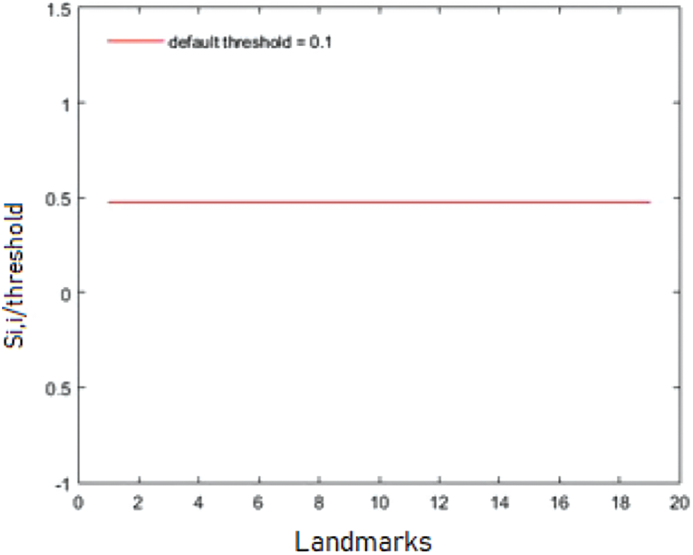
Figure 7: Abnormality visualization for a normal case
5.1.4 Results of Images with Dysmorphisms
Fig. 8 shows a malformation case III with the clear protrudent mandible compared to the maxilla. The correspondence between the model and the test cephalometric landmarks was achieved.
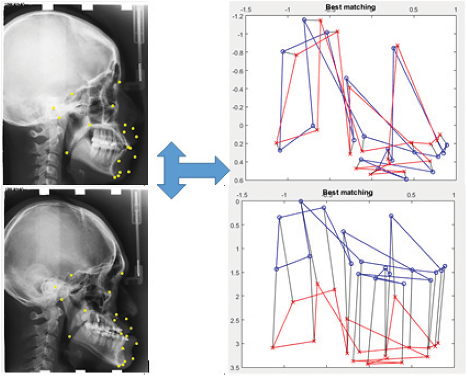
Figure 8: Landmarks matching results in the case of an abnormality class III
5.1.5 S’ Similarity Matrix Between Matching Points
Now, let S’ be a matrix of dimensions <19 × 19> representing the similarity matrix for the specified descriptor, where S’ (i, j) is the similarity between i-th vertex/point of shape 1 and the j-th vertex/point of shape 2, e.g., 10.8182 mm is the distance between the first landmark of the model landmarks and the first landmark of the test landmarks. Tab. 5 displays the diagonal values of the Matrix. S’ in mm. The obtained matrix shows that the diagonal values are greater than zero, which proves the existence of malformations. The sigmoid function to the diagonal values provides the malformation profile shown in Fig. 9 where the greatest anomaly lies in landmark 10.
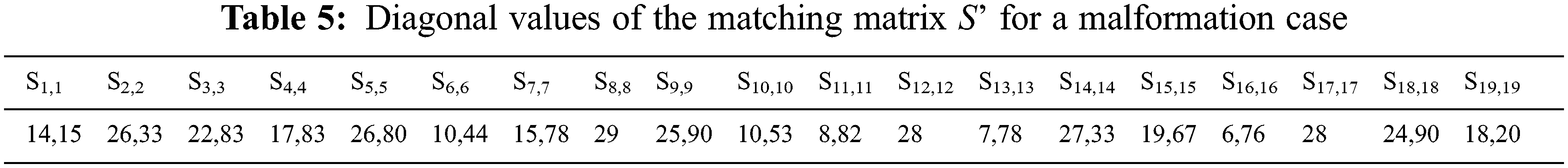
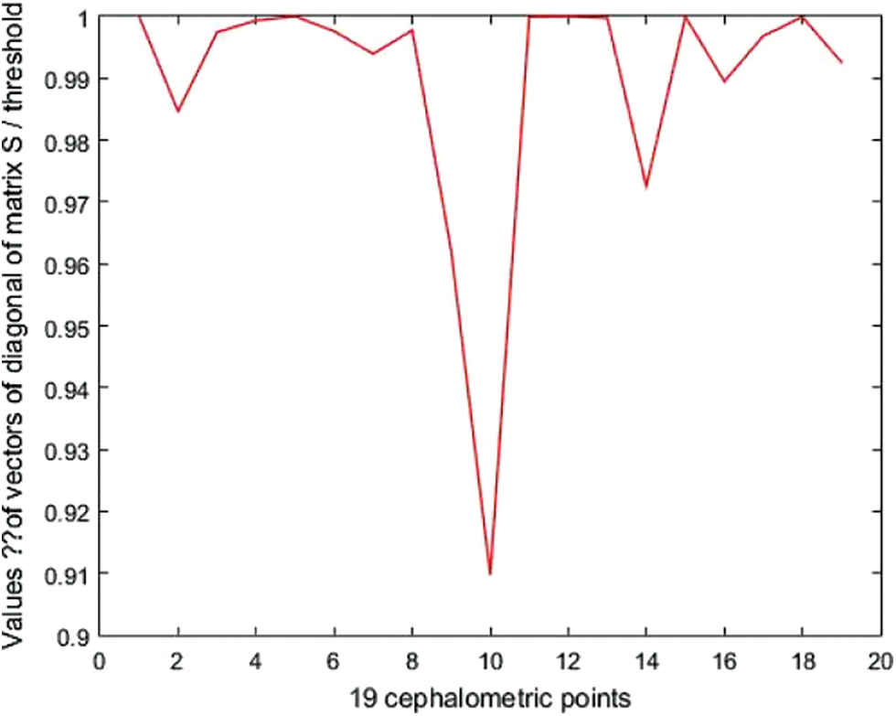
Figure 9: Abnormality profile for a case with anomalies
The developed framework was compared to the ground truth landmarks involving 250 test dataset. The matching matrix provides the difference between all the landmarks’ positions. Therefore, it provides a similarity measurement between landmarks. The given matrix is a quantitative measure of the matching of the 19 landmarks. Our framework showed a landmark matching error (LE) of 0.50 ± 1.04. It achieved a successful landmark matching of 89.47% in the 2 mm and 3 mm ranges and of 100% in the 4 mm range. The maximum matching distance is for the Gonion (3.43 mm).
For anomaly cases, the matching error is of 1.94 ± 0.78 mm. the successful landmark matching rate is 52,7%, 94.37% and 100% for respectively 2 mm, 3 mm and 4 mm. The proposed landmark approach reaches less performant results in the case of abnormality which is explained by the deformation impact on the natural landmark to the Bayesian convolutional neural networks presented in [41]. In this case, a deep architecture based on confidence region was proposed; the mean landmark error (LE) is 1.53 ± 1.74 mm and the detection rate is of 82.11%, 92.28% and 95.95% in respectively the 2 mm, 3 mm, and 4 mm ranges. Therefore, the proposed approach performs better matching results.
5.2 Anomalies Classification Using the SVM and KNN
The classification of the Maxillofacial anomalies with the SVM and KNN was detailed in this subsection. The different detailed classes in Tab. 6 were considered.
The dataset contains 284 samples for Class II and 114 samples for Class III. We took into account the maxillofacial anomalies labels Class II and Class III. The dataset was divided into two subsets as follows: an 80% training set involving 319 subjects and a 20% testing set including 79 subjects. The SVM classification results are shown in the Confusion Matrix in Fig. 10.
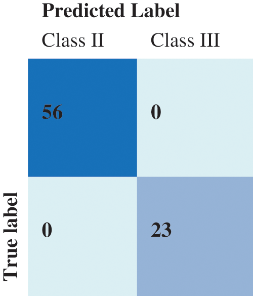
Figure 10: Confusion matrix of the SVM prediction results
For the KNN classification, the best result was obtained for k = 11, where k is the count of nearest neighbors as shown in Fig. 11. The Confusion Matrix in presented in Fig. 12.
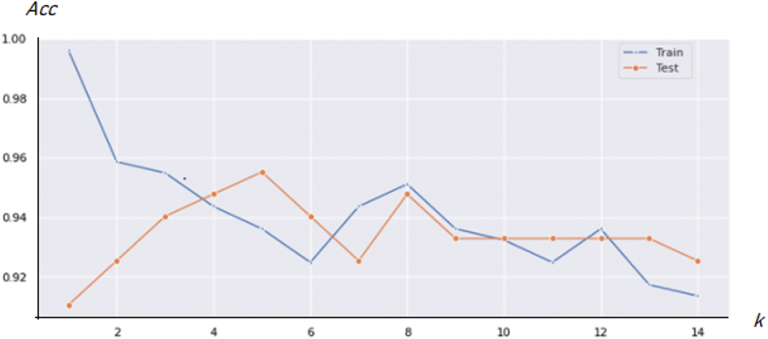
Figure 11: Best overall accuracy (Acc) for the KNN method variation for various k values
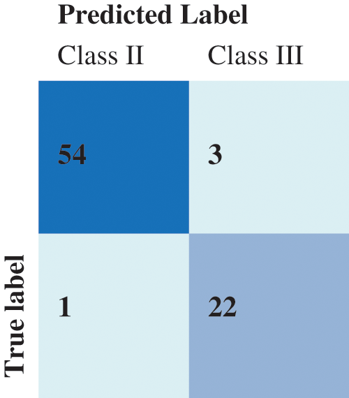
Figure 12: Confusion matrix of the KNN results
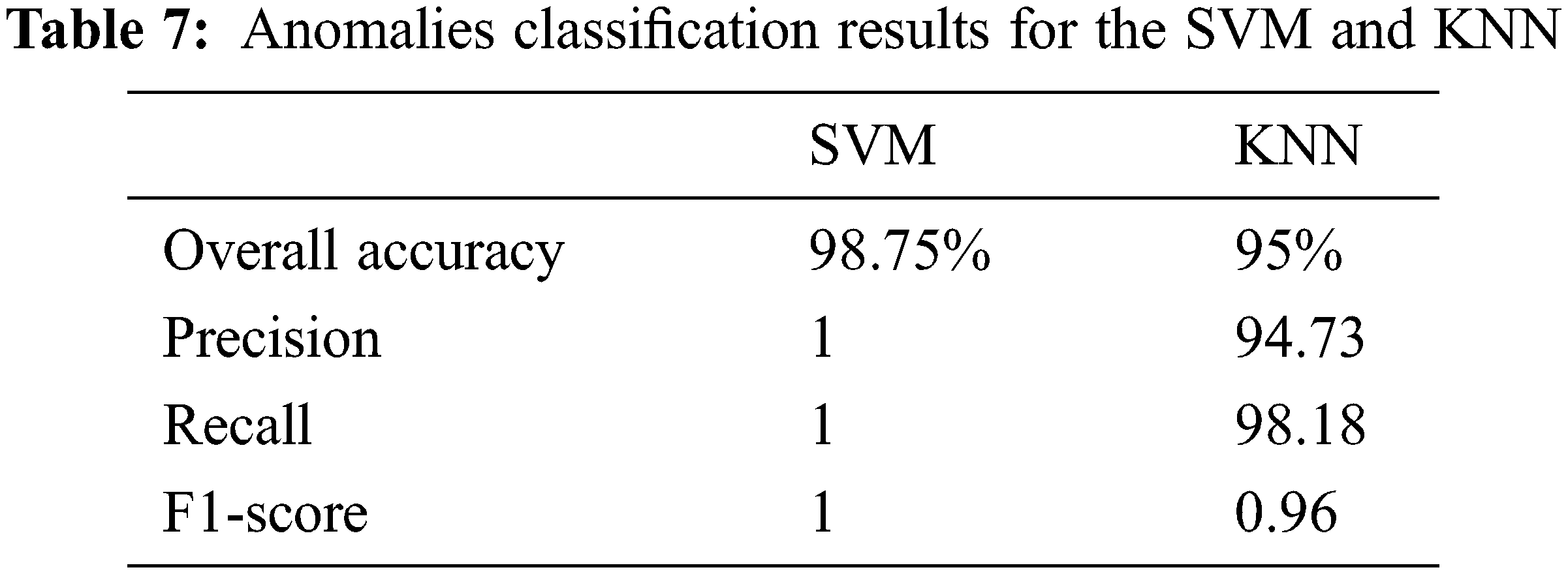
Tab. 7 details the classification metrics when considering class II and class III. The achieved accuracy is 98.75% for the SVM classifier and 95% when using the KNN classifier. The SVM resulted in a higher precision and recall than the KNN. It is crucial to reduce the prospect of getting false positives during such a prediction scenario as we do not want to mistakenly diagnose a patient with anomalies. The f1-score summarizes the classifier’s performance considering the Precision and Recall measures. Clearly, the SVM classifier reaches a better F1-score. Overall the proposed methodology for landmarks matching and anomalies classification has good performances and also significantly outperforms some cephalometric landmark detection methods. Existing techniques since the 2015 ISBI Grand Challenges followed a supervised learning approach and therefore are dependent on the learning process and data. In our case, the proposed QAP-based ACO framework is flexible when it comes to the number of landmarks and the order-preservation. It can be extended to 3D landmarks matching by determining the proximities over a surface. The limitations are related to the ACO itself when many constraints exist and less a priori information is available.
The proposed approach may be applied to a variety of fields for digital and clinical research. The adaptive control should be enhanced by experts within a knowledge-based dataset. The activation conditions can be applied by medical requirements or cephalometric x-ray images diagnosis. Compared to the other existing methods [9,32,33], it can be deduced that our contribution is original as a fully implementable approach for landmarks matching. Moreover, it proposed a malformation classification using the SVM. Further improvements of landmarks matching could be sought through the use of the matching results for the malformation quantification and preoperative planning. The framework could also take advantage form the machine learning [42], neural networks [43] and optimized deep architecture [44].
In this study, we proposed an automatic preoperative methodology of maxillofacial surgery, by performing a fully automatic cephalometric landmark matching and anomaly detection. The matching is based on constructing an AA model and then performing an ACO optimization. The maxillofacial anomalies are classified using the SVM. The achieved results show that our approach is promising and has lower computational cost. The system can be used for a fully automatic landmark matching and anomaly recognition, which allows an extensive cephalometric analysis. It introduced a computer aided diagnosis system that can be used within a digital clinic and assist clinical research for developing new treatments. The proposed approach has a low complexity and comparable landmark matching cost. Based on 2D imaging only, the approach provides landmark matching, graphic visualization of abnormality and anomality classification. Future works may include extending the system to an automatic landmark detection. It would be interesting to investigate the correlation between landmarks matching and clinical outcomes as well.
Acknowledgement: The authors would like to acknowledge the Princess Nourah bint Abdulrahman University Researchers Supporting Project number (PNURSP2022R196), Princess Nourah bint Abdulrahman University, Riyadh, Saudi Arabia.
Funding Statement: This work is supported by Princess Nourah bint Abdulrahman University Researchers Supporting Project number (PNURSP2022R196), Princess Nourah bint Abdulrahman University, Riyadh, Saudi Arabia.
Conflicts of Interest: The authors declare that they have no conflicts of interest to report regarding the present study.
1. M. Caihong, Z. Jian, L. Yi, Q. Rong and H. Tianhuan, “Multi-objective ant colony optimization algorithm based on decomposition for community detection in complex networks,” Soft Computing, vol. 23, no. 23, pp. 12683–12709, 2019. [Google Scholar]
2. T. V. Khmara, N. B. Kuzniak, Y. A. Morarash, M. O. Ryznychuk, A. Y. Petriuk et al., “Ontology of variants of cranial structure and malformations,” American Journal of Medical Genetics. Part C, Seminars in Medical Genetics, vol. 1, no. 4, pp. 232–245, 2013. [Google Scholar]
3. J. D. Bennett, “Preoperative preparation and planning of the oral and maxillofacial surgery patient,” Oral and Maxillofacial Surgery Clinics of North America, vol. 29, no. 2, pp. 131–140, 2017. [Google Scholar]
4. A. Kaur and C. Singh, “Automatic cephalometric landmark detection using zernike moments and template matching,” Signal Image Video Process, vol. 29, no. 1, pp. 117–132, 2015. [Google Scholar]
5. V. Grau, M. Alcaniz, M. C. Juan, C. Monserrat and C. Knol, “Automatic localization of cephalometric landmarks,” Journal of Biomedical Information, vol. 34, no. 3, pp. 146–156, 2001. [Google Scholar]
6. J. T. L. Ferreira and C. S. Telles, “Evaluation of the reliability of computerized profile cephalometric analysis,” Brazilian Dental Journal, vol. 13, no. 3, pp. 201–204, 2002. [Google Scholar]
7. Y. Weining, D. Yin, C. Li, G. Wang and X. Tianmin, “Automated 2-D cephalometric analysis on X-ray images by a model-based approach,” IEEE Transaction of Biomedical Engineering, vol. 13, no. 8, pp. 1615–1623, 2006. [Google Scholar]
8. S. Wang, H. Li, J. Li, Y. Zhang and B. Zou, “Automatic analysis of lateral cephalograms based on multiresolution decision tree regression voting,” Journal of Healthcare Engineering, vol. 15, no. 1, pp. 1–15, 2018. [Google Scholar]
9. C. Lindner, C. W. Wang, C. T. Huang, C. H. Li, S. W. Chang et al., “Fully automatic system for accurate localization and analysis of cephalometric landmarks in lateral cephalograms,” Scientific Reports, vol. 6, no. 33581, pp. 1–10, 2016. [Google Scholar]
10. H. Elmannai, M. Hamdi and A. AlGarni, “Deep learning models combining for breast cancer histopathology image classification,” International Journal of Computational Intelligence Systems, vol. 14, no. 1, pp. 1003–1013, 2021. [Google Scholar]
11. H. Lee, M. Park and J. Kim, “Cephalometric landmark detection in dental x-ray images using convolutional neural networks,” in Proc. of Medical Imaging: Computer-Aided Diagnosis, Orlando, USA, pp. 101341W, 2017. [Google Scholar]
12. S. O. Arik, I. Bulat and X. T. Lei, “Fully automated quantitative cephalometry using convolutional neural networks,” Journal of Medical Imaging, vol. 4, no. 1, pp. 014501, 2017. [Google Scholar]
13. J. Qian, M. Cheng, Y. Tao, J. Lin and H. Lin, “CephaNet: an improved Faster R-CNN for cephalometric landmark detection,” in Proc. of the IEEE Int. Symp. on Biomedical Imaging, Venice, Italy, pp. 868–871, 2019. [Google Scholar]
14. Y. Song, X. Qiao, Y. Wamoto and Y. W. Chen, “Automatic cephalometric landmark detection on x-ray Images using a deep-learning method,” Applied Sciences, vol. 10, no. 7, pp. 2547, 2020. [Google Scholar]
15. B. Ibragimov, B. Likar, F. Pernus and T. Vrtovec, “Computerized cephalometry by game theory with shape-and appearance-based landmark refinement,” in Proc. of the IEEE Int. Symp. on Biomedical Imaging, New York, USA, pp. 1–8, 2015. [Google Scholar]
16. O. Sercan, B. Ibragimov and L. Xing, “Fully automated quantitative cephalometry using convolutional neural networks,” Journal of Medical Imaging, vol. 4, no. 1, pp. 014501, 2017. [Google Scholar]
17. S. Ren, K. He, R. Girshick and J. Sun, “Faster r-cnn: Towards real-time object detection with region proposal networks,” in Proc. of the Conf. on Neural Information Processing Systems, Montréal, Canada, pp. 91–99, 2015. [Google Scholar]
18. B. H. Broadbent, “A new x-ray technique and its application to orthodontia,” The Angle Orthodontist, vol. 22, pp. 45–66, 1931. [Google Scholar]
19. M. Zeng, Z. Yan, S. Liu, Y. Zhou and L. Qiu, “Cascaded convolutional networks for automatic cephalometric landmark detection,” Medical Image Analysis, vol. 68, no. 1, pp. 101904, 2021. [Google Scholar]
20. S. H. Kang, K. Jeon, S. H. Kang and S. H. Lee, “3D cephalometric landmark detection by multiple stage deep reinforcement learning,” Scientific Reports, vol. 11, no. 17509, pp. 419, 2021. [Google Scholar]
21. S. Ghosh, A. Dasgupta and A. Swetapadma, “A study on support vector machine based linear and non-linear pattern classification,” in Proc. of the IEEE Int. Conf. on Information Systems Security, Tokyo, Japan, pp. 24–28, 2019. [Google Scholar]
22. M. Amrane, S. Oukid, I. Gagaoua and T. Ensar, “Breast cancer classification using machine learning,” in Proc. of the IEEE Scientific Meeting on Electrical- Electronics, Computer Science, Biomedical Engineering, Istanbul, Turkey, pp. 1–4, 2018. [Google Scholar]
23. G. V. Batista, T. Scarpin and E. Pécora, “A new ant colony optimization algorithm to solve the periodic capacitated arc routing problem with continuous moves,” Mathematical Problems in Engineering, vol. 2019, no. 1, pp. 1–13, 2019. [Google Scholar]
24. C. Mu, J. Zhang and Y. Liu, “Multi-objective ant colony optimization algorithm based on decomposition for community detection in complex networks,” Soft Computing, vol. 23, no. 23, pp. 12683–12709, 2019. [Google Scholar]
25. H. L. D. Silveira, M. J. Gomes, H. E. D. Silveira and R. R. Dalla-Bona, “Evaluation of the radiographic cephalometry learning process by a learning virtual object,” American Journal of Orthodontics and Dentofacial Orthopedics, vol. 136, no. 1, pp. 134–138, 2009. [Google Scholar]
26. X. Hu, P. Luo, X. Zhang and J. wang, “Improved ant colony optimization for weapon-target assignment,” Mathematical Problems in Engineering, vol. 14, no. 3, pp. 1–14, 2018. [Google Scholar]
27. A. Agharghor, M. E. Rifi and F. Chbihi, “Improved hunting search algorithm for the quadratic assignment problem,” Indonesian Journal of Electrical Engineering and Computer Science, vol. 14, no. 1, pp. 143–154, 2019. [Google Scholar]
28. V. Sergienko, V. P. Shylo, S. V. Chipov and P. V. Chylo, “Solving the quadratic assignment problem,” Cybernetics and Systems Analysis, vol. 56, no. 1, pp. 53–57, 2020. [Google Scholar]
29. M. Dorigo, M. Birattari and T. Stutzle, “Ant colony optimization,” IEEE Computational Intelligence Magazine, vol. 1, no. 4, pp. 28–39, 2006. [Google Scholar]
30. D. B. Ismail, K. Aloui and M. S. Naceur, “Matching cephalometric points via Ant Colony Optimization,” in Proc. of the IEEE Conf. on Advances in Science and Engineering Technology, Dubai, United Arab Emirates, pp. 289–293, 2020. [Google Scholar]
31. P. Pardalos, F. Rendl and H. Wolkowicz, “The quadratic assignment problem: A survey and recent developments. in quadratic assignment and related problems,” American Mathematical Science, vol. 41, pp. 1–42, 1994. [Google Scholar]
32. H. Chui and A. Rangaragan, “A new point matching algorithm for non-rigid registration,” Computer Vision and Image Understanding, vol. 89, no. 2-3, pp. 114–141, 2003. [Google Scholar]
33. A. Nayyar and R. Singh, “Ant colony optimization—computational swarm intelligence technique,” in Proc. of the IEEE Conf. on Computing for Sustainable Global Development, New Delhi, India, pp. 1493–1499, 2016. [Google Scholar]
34. R. Armand, B. William and F. Punch, “Genetic programming for tuberculosis screening from raw x-ray images,” in Proc. of the Conf. on Genetic and Evolutionary Computation, Kyoto, Japan, pp. 1214–1221, 2018. [Google Scholar]
35. D. B. Ismail, K. Aloui and J. Bouguila, “Preoperative planning tools for mandibular reconstruction,” in Proc. of the Conf. on Advanced Systems and Electric Technologies, Hammamet, Tunisia, pp. 60–65, 2017. [Google Scholar]
36. V. Maniezz and A. Colorni, “The ant system applied to the quadratic assignment problem,” IEEE Transaction on Knowledge and Data Engineering, vol. 5, no. 5, pp. 769–778, 1999. [Google Scholar]
37. A. C. Berg, T. L. Berg and J. Malik, “Shape matching and object recognition using low distortion correspondences,” in Proc. of the IEEE Computer Society Conf. on Computer Vision and Pattern Recognition, San Diego, USA, pp. 26–33, 2005. [Google Scholar]
38. H. Elmannai, M. A. Loghmari and M. S. Naceur, “Support vector machine for remote sensing image classifications,” in Proc. of the Conf. on Control, Engineering & Information Technology, Sousse, Tunisia, pp. 68–72, 2013. [Google Scholar]
39. H. Elmannai, M. A. Loghmari and M. S. Naceur, “A new classification approach based on source separation and feature extraction,” in Proc. pf the IEEE Symp. Signal, Image, Video and Communications, Tunis, Tunisia, pp. 137–141, 2016. [Google Scholar]
40. O. Sammoud, S. Sorlin, C. Solnon and K. Ghedira, “A comparative study of ant colony optimization and reactive search for graph matching problems,” Evolutionary Computation in Combinatorial Optimization, vol. 13, pp. 234–246, 2006. [Google Scholar]
41. J. H. Lee, H. J. Yu, M. Kim, J. W. Kim and J. Choi, “Automated cephalometric landmark detection with confidence regions using bayesian convolutional neural networks,” BMC Oral Health, vol. 20, no. 1, pp. 270, 2020. [Google Scholar]
42. J. Alzubi, A. Nayyar and A. Kumar, “Machine learning from theory to algorithms: An overview,” Journal of Physics: Conference Series, vol. 1142, no. 1, pp. 012012, 2018. [Google Scholar]
43. X. R. Zhang, X. Sun, W. Sun, T. Xu and P. P. Wang, “Deformation expression of soft tissue based on BP neural network,” Intelligent Automation & Soft Computing, vol. 32, no. 2, pp. 1041–1053, 2022. [Google Scholar]
44. X. R. Zhang, X. Chen, W. Sun and X. Z. He, “Vehicle re-identification model based on optimized denseNet121 with joint loss,” Computers Materials & Continua, vol. 67, no. 3, pp. 3933–3948, 2021. [Google Scholar]
 | This work is licensed under a Creative Commons Attribution 4.0 International License, which permits unrestricted use, distribution, and reproduction in any medium, provided the original work is properly cited. |