DOI:10.32604/iasc.2023.029602
| Intelligent Automation & Soft Computing DOI:10.32604/iasc.2023.029602 | |
| Article |
A Novel Handcrafted with Deep Features Based Brain Tumor Diagnosis Model
1Department of Documents and Archive, Center of Documents and Administrative Communication, King Faisal University, Al Hofuf, 31982, Al-Ahsa, Saudi Arabia
2School of Electrical and Electronic Engineering, Engineering Campus, Universiti Sains Malaysia (USM), Nibong Tebal, 14300, Penang, Malaysia
*Corresponding Author: Abdul Rahaman Wahab Sait. Email: asait@kfu.edu.sa
Received: 07 March 2022; Accepted: 14 April 2022
Abstract: In healthcare sector, image classification is one of the crucial problems that impact the quality output from image processing domain. The purpose of image classification is to categorize different healthcare images under various class labels which in turn helps in the detection and management of diseases. Magnetic Resonance Imaging (MRI) is one of the effective non-invasive strategies that generate a huge and distinct number of tissue contrasts in every imaging modality. This technique is commonly utilized by healthcare professionals for Brain Tumor (BT) diagnosis. With recent advancements in Machine Learning (ML) and Deep Learning (DL) models, it is possible to detect the tumor from images automatically, using a computer-aided design. The current study focuses on the design of automated Deep Learning-based BT Detection and Classification model using MRI images (DLBTDC-MRI). The proposed DLBTDC-MRI technique aims at detecting and classifying different stages of BT. The proposed DLBTDC-MRI technique involves median filtering technique to remove the noise and enhance the quality of MRI images. Besides, morphological operations-based image segmentation approach is also applied to determine the BT-affected regions in brain MRI image. Moreover, a fusion of handcrafted deep features using VGGNet is utilized to derive a valuable set of feature vectors. Finally, Artificial Fish Swarm Optimization (AFSO) with Artificial Neural Network (ANN) model is utilized as a classifier to decide the presence of BT. In order to assess the enhanced BT classification performance of the proposed model, a comprehensive set of simulations was performed on benchmark dataset and the results were validated under several measures.
Keywords: Brain tumor; medical imaging; image classification; handcrafted features; deep learning; parameter optimization
Abnormal development of cells in brain causes Brain Tumors (BT) which tend to affect any individual irrespective of the age. BTs have been diagnosed to have different sizes and shapes while their image intensities arise at any location [1]. BT classification is a primary stage in healthcare sector. The image attained from distinct modalities must be verified by a medical doctor so that they can suggest for alternative treatments. However, manual classification of Magnetic Resonance Imaging (MRI) is a time consuming and challenging task [2,3]. Human observation might also result in misclassification due to which it is necessary for semiautomatic or automatic classifier methods to differentiate among dissimilar types of tumor [4]. Deep Learning (DL) is a kind of Artificial Intelligence (AI) method that simulates the functions of individual brain through data processing and generates prototypes that are valuable in making appropriate selections. DL calculation utilizes different nonlinear layers that are systematic to extract features from the image [5]. The results of each ordered layer influence the subsequent layers and it also assists in data deliberation.
In literature [6], deep CNN was initially proposed as a DL network ‘LeNet’ to identify the documents. In the past few years, it considerably expanded while employing a DL method that is exploited for identification of images using a pretrained network (PTN) named AlexNet [7,8]. It yielded outstanding results than other methods. Next, its prosperity encouraged back-to-back achievements of Convolution Neural Network (CNN) in the field of DL. The major point of interest in CCNN is its capability to learn features and provide boundless accuracy against traditional AI approaches. This can be achieved by increasing the number of instances utilized for training purposes. Thus, it had evolved as a precise and very effective model [9,10]. Khan et al. [11] projected an automated multi-modal classifier technique utilizing DL for classification of BT types. The presented technique comprises of five core stages. In primary stage, linear contrast stretching was done utilizing edge-based histogram equalization and Discrete Cosine Transform (DCT). In the secondary stage, DL feature extraction was done. By employing Transfer Learning (TL), two pre-trained CNN techniques such as VGG16 and VGG19 were utilized for feature extraction. In the tertiary stage, a cross-entropy based joint learning method was executed together with Extreme Learning Machine (ELM) for the chosen optimum features.
Kumar et al. [12] presented a DL method utilized ResNet-50 and global average pooling so as to resolve the vanishing gradient and overfitting problem. In order to establish the efficacy of the presented method, simulation was performed using a 3-tumor brain MRI data set containing 3,064 images. In [13], an MRI-based non-invasive BT grading technique was presented utilizing DL and Machine Learning (ML) approaches. Four datasets were used for training and testing purposes on five DL-based techniques like VGG16, ResNet50, AlexNet, ResNet18, and GoogleNet, and five ML-based methods utilizing 5-fold cross validation. A majority voting (MajVot)-based ensemble technique was presented to optimize the entire classifier performance of 5 DL and 5 ML-based techniques.
In literature [14], the ML approaches that exist in research data were discussed and listed for improving the performance and overcoming the limitation of medicinal image analytics. An important purpose of this review is to grasp the overview of the demonstrated approaches that offer optimum BT dissect. BT classification undergoes various stages before attaining the fulfilled outcomes in terms of classification and analysis, while the results help in treatment planning as radiotherapy. In literature [15], segmentation was completed by hybridizing the classical k-means technique with Swarm-based Grass Hopper Optimization (SGHO) technique. Speed Up Robust Feature (SURF) technique was executed to extract the features of BT image. In this study, SGHO-based approach was utilized to select the feature. In final stage, Support Vector Machine (SVM) technique was used to classify the tumor images.
In this background, the current study presents automated Deep Learning based BT Detection and Classification model using MRI images (DLBTDC-MRI). The proposed DLBTDC-MRI technique focuses on effective recognition and classification of various levels of BT. The proposed DLBTDC-MRI technique involves median filtering technique for noise removal so as to enhance the quality of MRI images. Besides, morphological operations-based image segmentation approach is applied to determine the BT-affected regions in brain MRI image. Moreover, a fusion of handcrafted deep features using VGGNet is utilized to derive a valuable set of feature vectors. Finally, Artificial Fish Swarm Optimization (AFSO) is utilized with Artificial Neural Network (ANN) as a classifier to decide the presence of BT. In order to validate the enhanced BT classification performance of the proposed model, a comprehensive set of simulations was conducted upon benchmark dataset and the outcomes were assessed under different measures.
Rest of the paper is organized as follows. Section 2 introduces the proposed model and Section 3 offers information on performance validation. Then, Section 4 concludes the work.
In this study, a novel DLBTDC-MRI technique has been developed for effectual identification and classification of various stages of BT. The workflow is given in Fig. 1. The proposed DLBTDC-MRI approach involves distinct stages namely, MF-based pre-processing, morphological segmentation, fusion-based feature extraction, ANN classification, and AFSO-based parameter optimization.
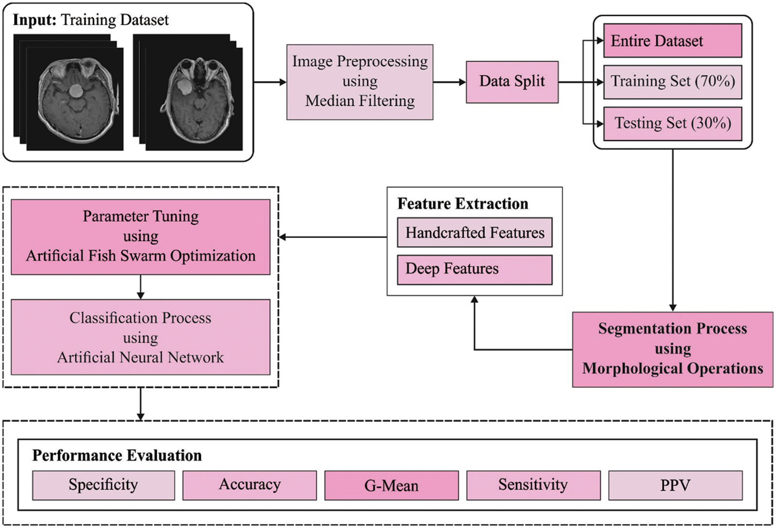
Figure 1: Workflow of DLBTDC-MRI model
2.1 Morphological Operations Based Segmentation
During segmentation stage, morphological operations are carried out to identify the affected tumor areas. Erosion and dilation are two basic functions in morphological image processing whereas all other morphological functions are based on these two functions [16]. Initially, it is determined upon binary images while later, it is extended for grayscale images also. In an image, when pixels are in addition to the boundaries of objects, it is named as dilation. On the contrary, once the pixels are removed from the boundary of object, it can be turned into erosion. Based on support of erosions and dilations, it can further design complicated morphological operators. With the help of a structural element (set) B on shape (set) A, the processing is completed.
During dilation, it can have the original set together with more boundaries. Both size and shape of the structural elements choose what will be the size and shape of boundaries. Erosion resolves, if the constructing element is present in the original set. The erosion process eliminates the outer boundary of the original shape. The relation between dilation and erosion is that both are complementary functions.
To a symmetric structural component, following is the equation
2.2 Fusion Based Feature Extraction
In feature extraction stage, handcrafted features are fused with deep features using VGGNet to derive a valuable set of feature vectors. Grey Level Co-occurrence Matrix (GLCM) model is generally observed as a matrix in which the row and column counts are equal to the count of gray level, G. The matrix component p(x, y|d1, d2) symbolizes the corresponding value separated by pixel distance (dl and d2). GLCM enables the gathering of adequate statistics with respect to grey co-props function that offers the texture detail of the image namely, energy, entropy, contrast, correlation, and homogeneity. VGG-16 is a familiar DL model thanks to its regular structure and better performance in classification process [17]. It includes 16 trainable layers comprising 13 convolution layers and 3 fully-connected layers. The convolution layer is assembled under five blocks. The nearby blocks are connected via max pooling layer that performs down-sampling by half, along with spatial dimension. The max-pooling layer minimizes the layer dimension from 224 × 224 in the initial block to 7 × 7 after the final block. The convolution filter count stays predefined in one block and gets doubled after every max-pooling layer. It is followed by Rectified Linear Unit (ReLU) and Fully Connected (FC) layers.
At last, the optimal ANN model is used to classify the BT under different stages. ANN is comprised of processing element that is analogous to synapses and is highly interconnected [18]. This highly-connected processing element is named an ‘artificial neuron’. Artificial neurons can be activated by evaluating the input and weights through an arithmetic equation. ANN contains intermediate layers between input and output layers that are represented as hidden nodes whereas they possess hidden node embedded in them. Therefore, the resultant structure is called Multilayer Neural Network (MLNN) and the node in one layer is interconnected with the node in the following layer. The structure of ANN follows a multi-layer Feed Forward Neural Network (FFNN). Multilayer FFNN contains input, hidden, and output nodes. The output received from the input layer is passed on to output layer, once it is computed and processed in hidden node. The inherent model of neural networks makes it an effective mechanism to process complicated datasets as in breast cancer research which is represented as non-linear interactions between target and input prediction. Multilayer FFNN is trained by Backpropagation (BP) approach and is widely employed for pattern classification, since they learn to transform the input information. The backpropagation of error from output node to the hidden node is the major concept of this method. BPNN denotes a neuron and adjacent layer that are interconnected by weights. It can be formulated through the following equation.
Whereas, fj denotes the activation function, wji represents the weight related to connections between nodes in input neuron i and hidden neuron j, aj indicates the bias related to connections between input and hidden layers, γi denotes the input at nodes in input layer, Ij represents the summation of weight input added with bias, and Yj implies the output of activation function at hidden layer. The principle of output layer is deduced using the following equation,
where fn refers to activation function, wnj indicates the weight related to connections between nodes in hidden layer j and output layer n, and bn represents the bias related to connections between hidden and output layers. Besides, yj signifies the output at nodes in hidden node and In summation indicates the weight of the output at output layer. It is significant to note that i represents the input node, j denotes the hidden node and n indicates the output node.
In order to optimally adjust the parameters involved in ANN model, AFSO algorithm is applied. In water, fishes are found dispersed from one place to another, where food is available and simultaneously stay closer to the swarm. Fish endlessly alters its location in a swarm based on its own state and external environment [19]. Though the movement of fish in a swarm seems to be random, it is actually a highly synchronized movement that suits the objectives. They remain closer to the swarm to protect itself from the predators, keep safe distance from neighboring fishes to continuously search for food and prevent collision. This behavior stimulated the development of a new algorithm to resolve optimization problems with a considerable number of efficiencies. The method employs a local search behavior of individual fish, called artificial fish so as to reach the global optimum solution. Swarming, random search, preying, and following behaviors of the fishes are adapted for this search. The process involved in AFSO algorithm is given in Fig. 2. The location of the artificial fish signifies a likely solution. The existing location xi is denoted by Xi = (xi1, xi2 … xin) whereas i denotes the amount of control parameters and n indicates the amount of fish. The consistency of the food, which the artificial fish could identify in location xi, is shown as Yi = f(Xi). The novel location of the artificial
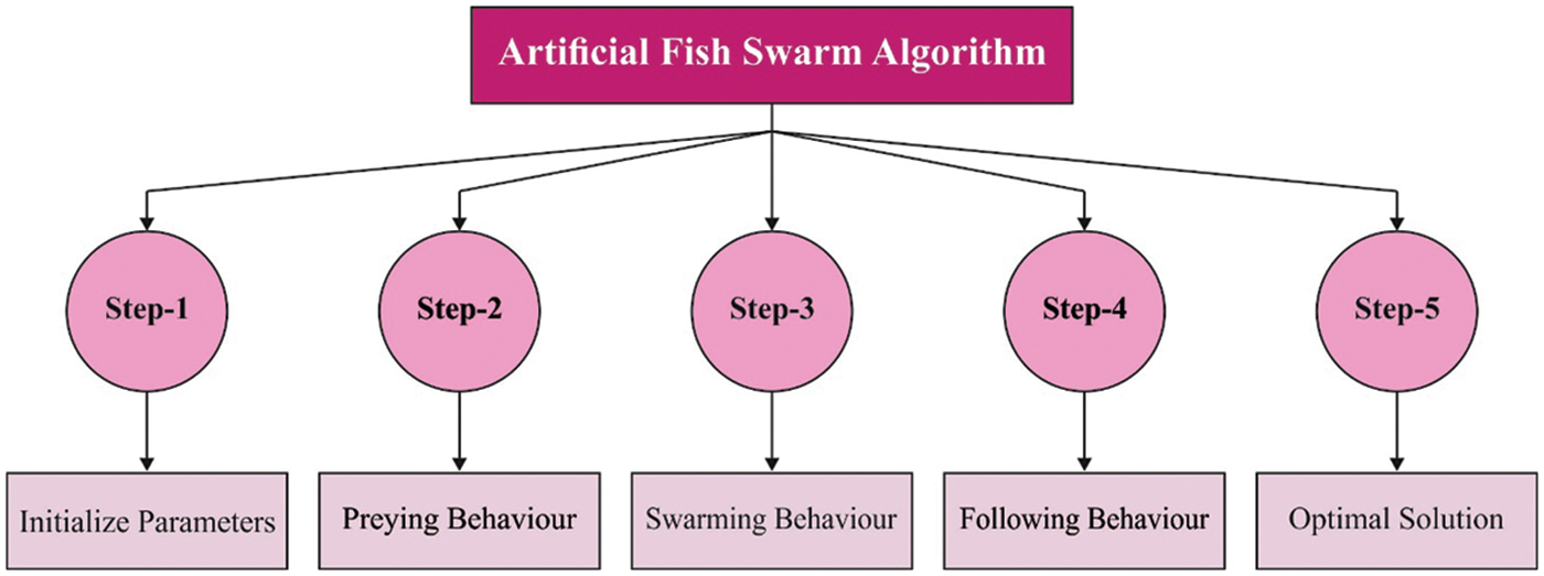
Figure 2: Process involved in AFSO algorithm
Whereas rand() denotes an arbitrary value between 0−1, step indicates the distance where a fish moves in one movement, Xj indicates the location within the scope of vision of the fish. The location Xj can be determined under distinct behaviors of fish as discussed herewith.
Chasing the trail behavior: The artificial fish follows the neighboring fish, i.e., located at a place with further food consistency in their vision scope to find more food. Now Xj denotes the location of the neighbour.
Gathering or Swarming behavior: The artificial fish has a propensity to move to the center of the swarm so as to ensure the existence of swarm around it and prevent itself from potential danger. Now Xj is shown as follows.
Whereas Xc denotes the center of the swarm.
Preying or Foraging behavior: The artificial fish senses the food consistency at another location through sense or vision and defines the movement. Once it finds a position with further food everywhere, it straightaway travels in that direction. The location Xj in this behaviour can be shown as follows.
The aim of AFSO algorithm is to determine an objective function based on the fitness value of maximum classifier results with minimal error rate. The fitness function is offered in the following equation.
In order to establish the effective characteristics of the proposed DLBTDC-MRI model, a detailed experimental validation process was conducted using Figshare dataset [20]. It contains images under three classes and has a total of 150 images under Meningioma (MEN) class, 150 images under Glioma (GLI) class, and 150 images under Pituitary (PIT) class. Fig. 3 demonstrates some of the sample test images.
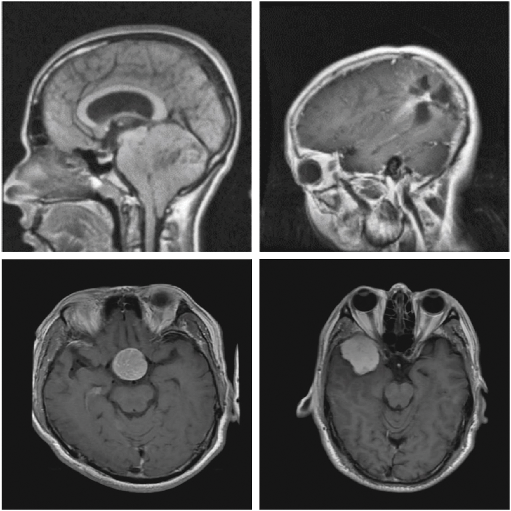
Figure 3: Sample images
Fig. 4 highlights the confusion matrices generated by the proposed DLBTDC-MRI model on test dataset. Fig. 4a indicates that the proposed DLBTDC-MRI model categorized 150 images under MEN, 146 images under GLI, and 147 images under PIT classes on the entire dataset. In addition, Fig. 4b reports that DLBTDC-MRI model categorized 101 images under MEN, 105 images under GLI, and 105 images under PIT classes on 70% of training dataset. Besides, Fig. 4c shows that the presented DLBTDC-MRI model classified 49 images under MEN, 41 images under GLI, and 42 images under PIT classes on 30% of testing dataset.
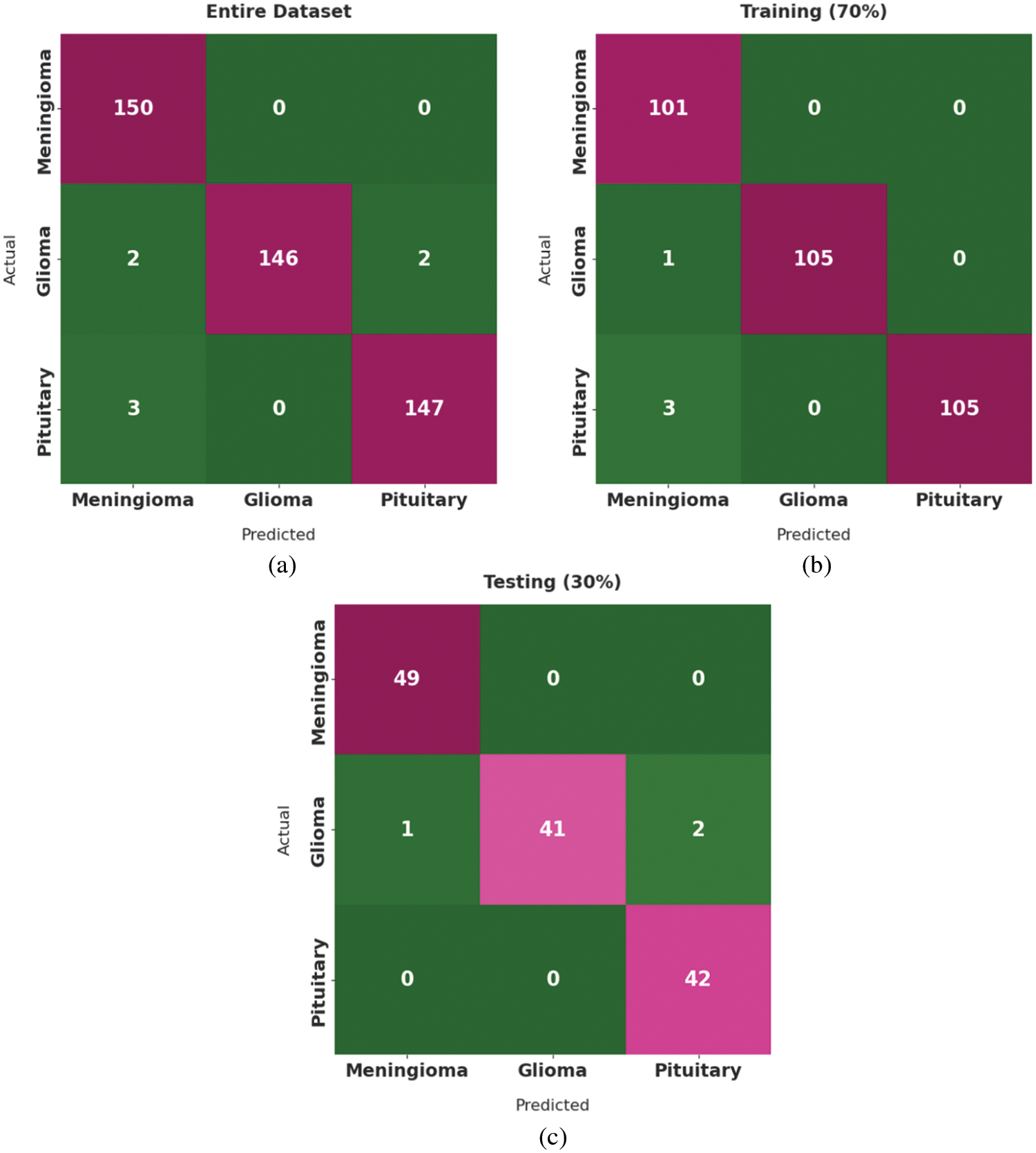
Figure 4: Confusion matrix of DLBTDC-MRI model: (a) Entire dataset, (b) 70% of training dataset and (c) 30% of testing dataset
Tab. 1 portrays the overall classification outcomes accomplished by the proposed DLBTDC-MRI model on distinct datasets. The table values report that DLBTDC-MRI model classified all the images under respective classes in an effective manner and achieved maximum classification performance.
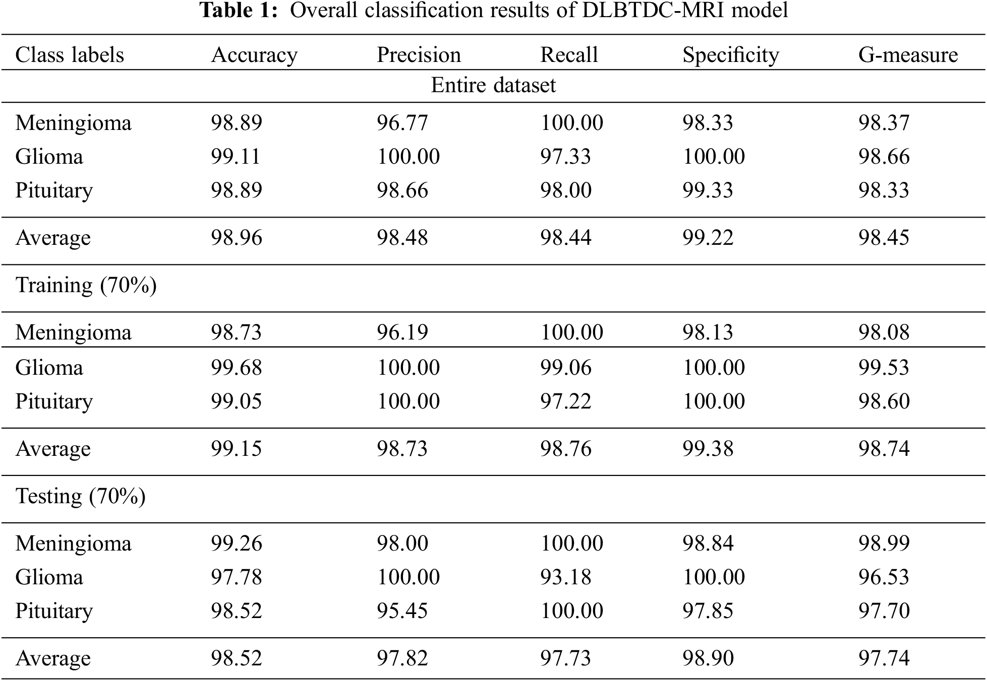
Fig. 5 briefs the average outcomes achieved from classification, performed by DLBTDC-MRI model on entire dataset. The figure indicates that the proposed DLBTDC-MRI model proficiently recognized the classes in the entire dataset with average accuy, precn, recal, specy, and Gmeasure values such as 98.96%, 98.48%, 98.44%, 99.22%, and 98.45% respectively.
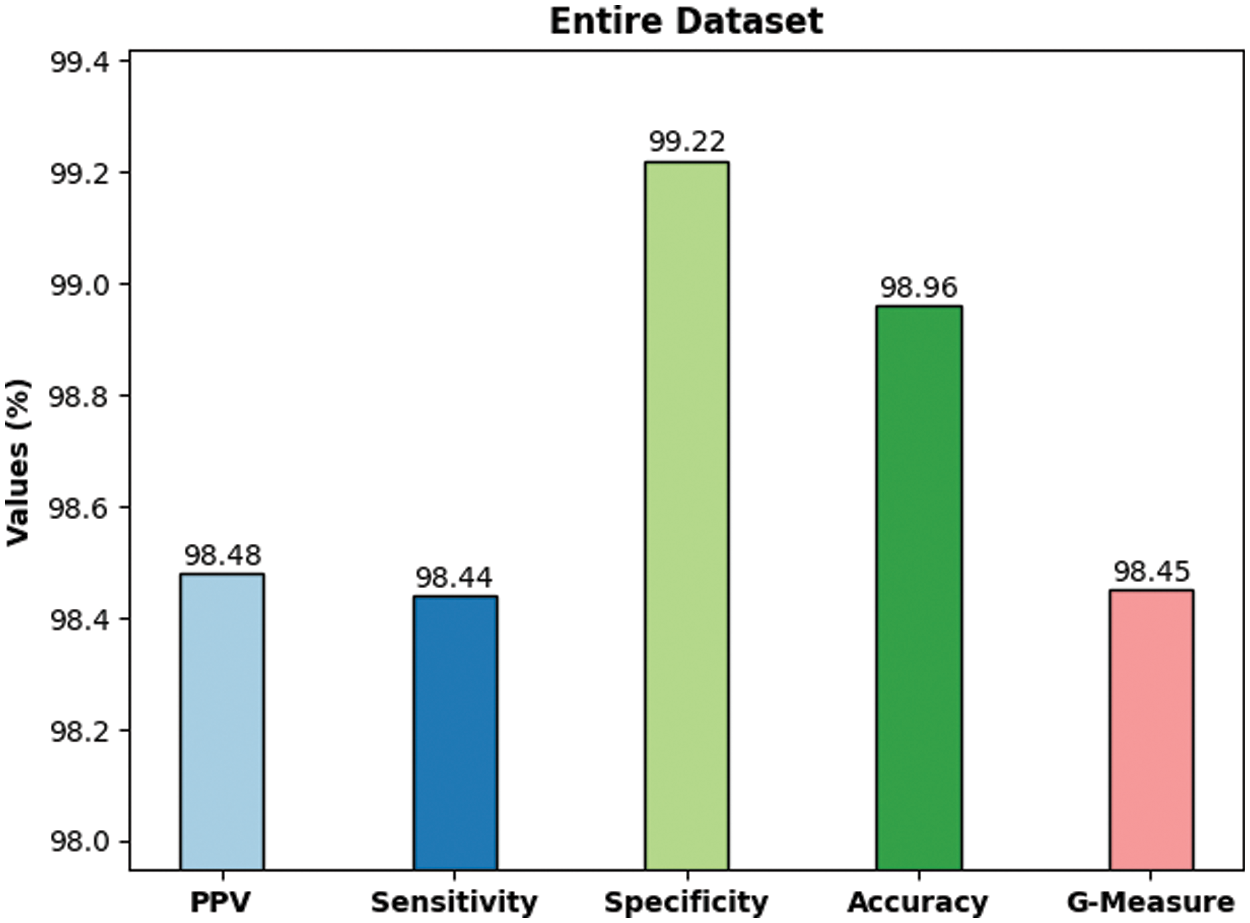
Figure 5: Classification outcomes of DLBTDC-MRI model on entire dataset
Fig. 6 shows the average classification outcomes attained by DLBTDC-MRI model on 70% training dataset. The figure shows that the proposed DLBTDC-MRI model proficiently acknowledged the classes in 70% of training dataset with average accuy, precn, recal, specy, and Gmeasure values such as 99.15%, 98.73%, 98.76%, 99.38%, and 98.74% respectively.
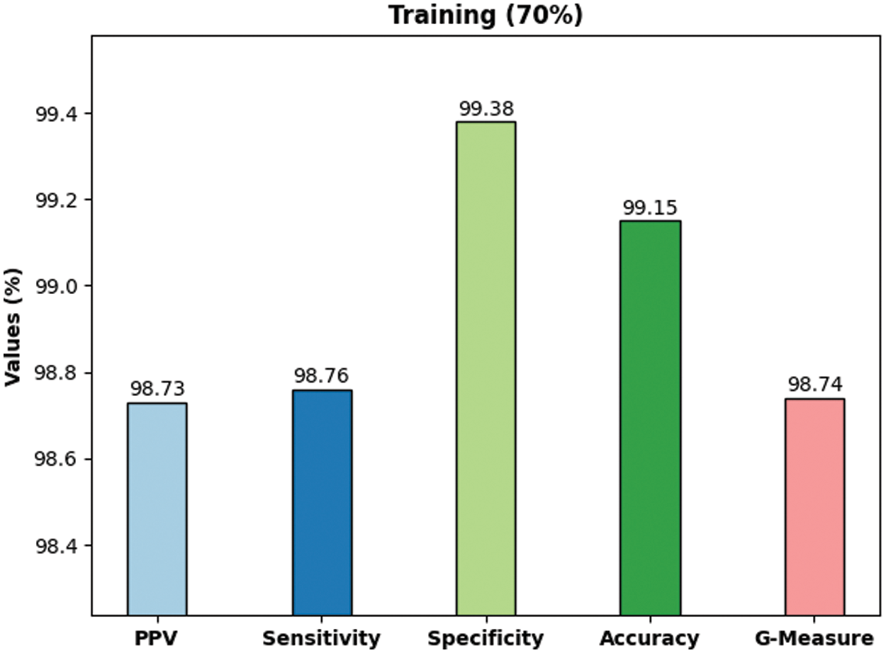
Figure 6: Classification outcomes of DLBTDC-MRI model on 70% of training dataset
Fig. 7 demonstrates the outcomes of average classification achieved by the proposed DLBTDC-MRI model on 30% testing dataset. The figure shows that the proposed DLBTDC-MRI model achieved a capable outcome on 30% testing dataset with average accuy, precn, recal, specy, and Gmeasure values such as 98.52%, 97.82%, 97.73%, 98.90%, and 97.74% respectively.
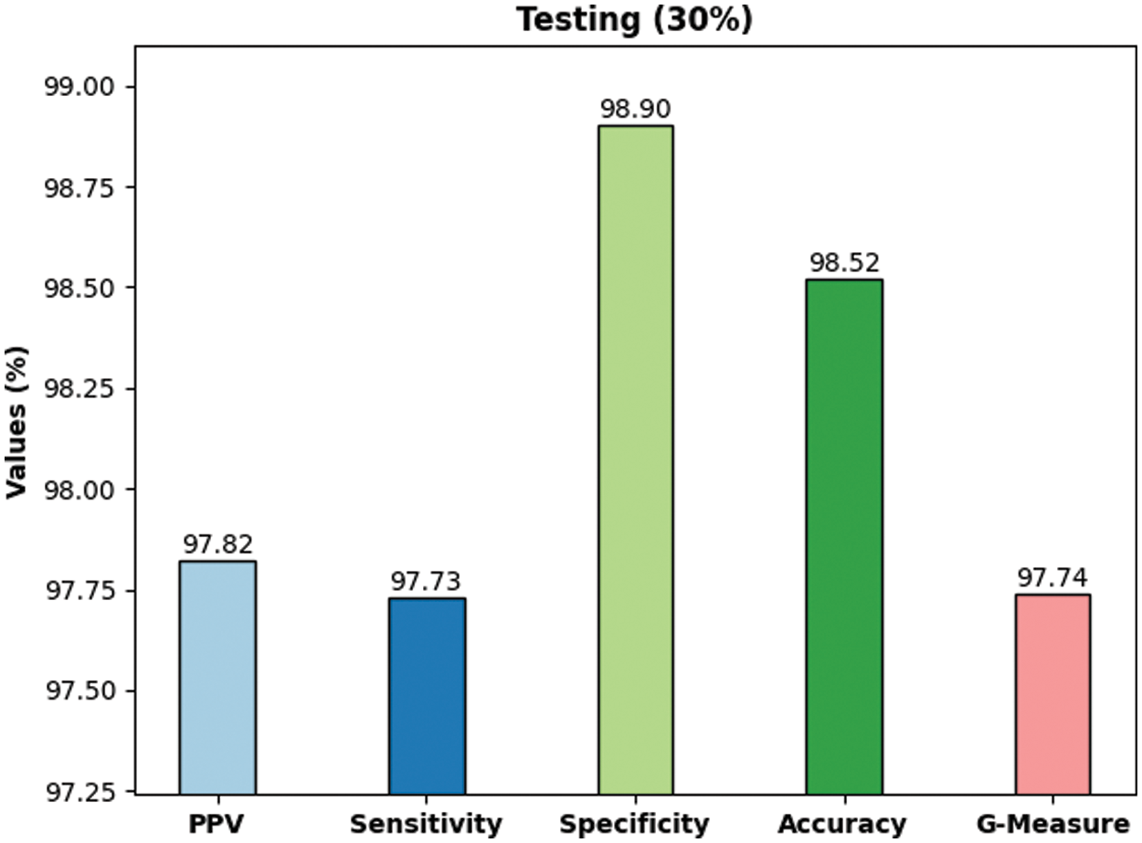
Figure 7: Classification outcomes of DLBTDC-MRI model on 30% of testing dataset
A brief precision-recall examination was conducted upon DLBTDC-MRI model using different forms of dataset and the results are portrayed in Fig. 8. By observing the figure, it can be understood that DLBTDC-MRI model accomplished the maximum precision-recall performance under all datasets.
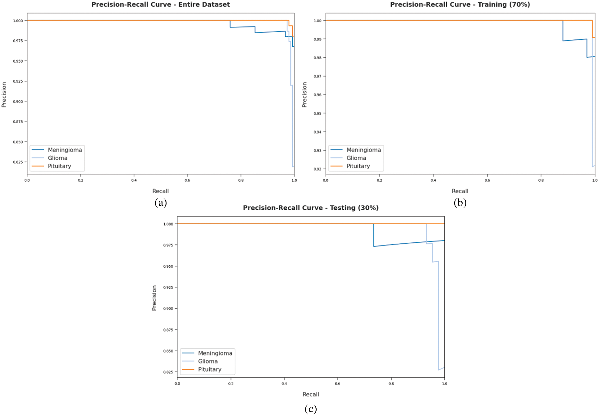
Figure 8: Precision-recall curves of DLBTDC-MRI model: (a) Entire dataset, (b) 70% of training dataset, (c) 30% of testing dataset
A detailed ROC investigation was conducted for DLBTDC-MRI model on distinct datasets and the results are showcased in Fig. 9. The results indicate that the proposed DLBTDC-MRI model exhibited its ability to categorize three different classes such as MEN, GLI, and PIT on test datasets.
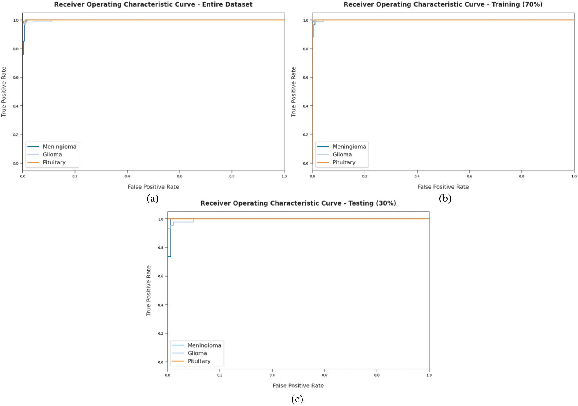
Figure 9: ROC of DLBTDC-MRI model: (a) Entire dataset, (b) 70% of training dataset and (c) 30% of testing dataset
Finally, a comparison study was conducted between DLBTDC-MRI model and existing models and the results are portrayed in Tab. 2 and Fig. 10. The experimental results indicate that CapsNets model offered a poor performance with sensy, specy, and accuy values such as 91.04%, 92.39%, and 90.89% respectively. Followed by, GLCM-Support Vector Machine (SVM) and CNN models resulted in slightly enhanced sensy, specy, and accuy values. Followed by, Kernel Extreme Learning Machine (KELM)-CNN model offered moderately improved sensy, specy, and accuy results such as 94.56%, 93.84%, and 93.68% respectively.
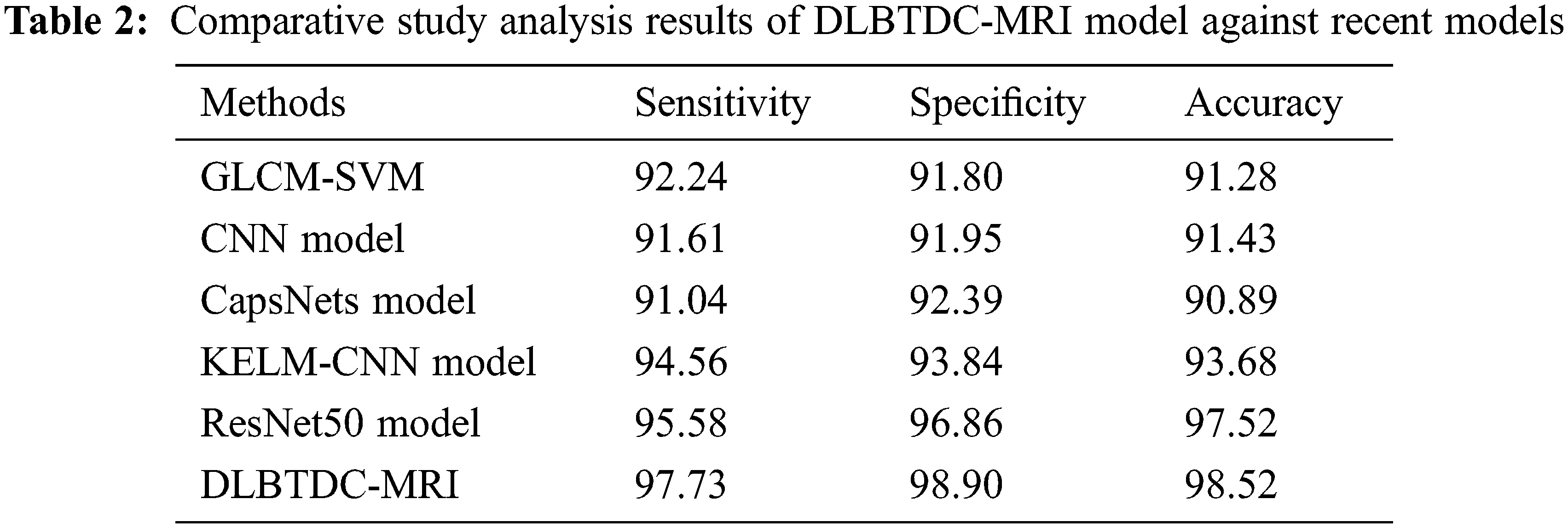
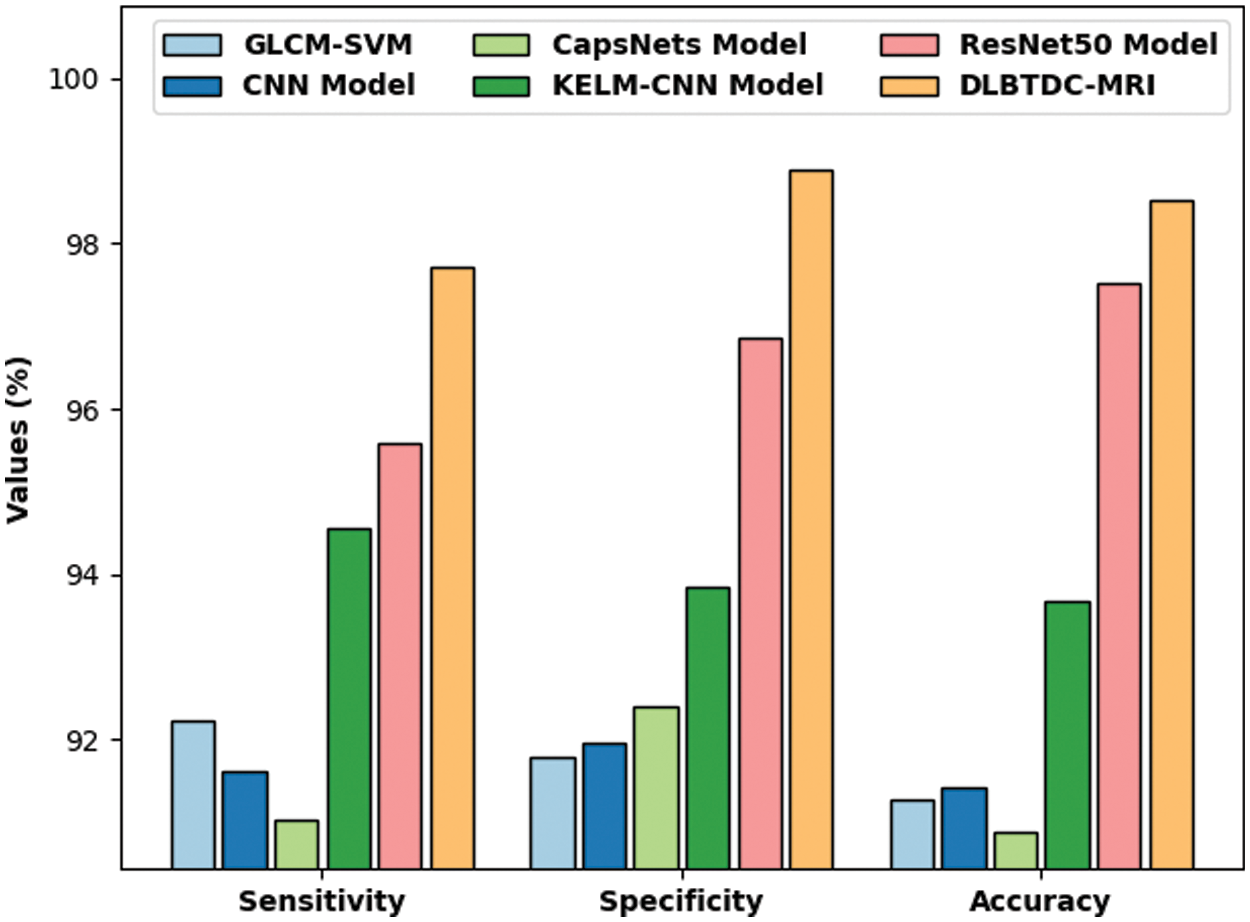
Figure 10: Comparison study results of DLBTDC-MRI model against recent models
Though ResNet50 model achieved reasonable outcomes in terms of sensy, specy, and accuy values such as 95.58%, 96.86%, and 97.52%, the proposed DLBTDC-MRI model accomplished an effectual outcome with maximum sensy, specy, and accuy values namely 97.73%, 98.90%, and 98.52%. After examining the above mentioned tables and figures, it is evident that the presented DLBTDC-MRI technique accomplished effectual outcomes.
In this study, a novel DLBTDC-MRI technique was developed for effectual identification and classification of various stages of BT. The proposed DLBTDC-MRI technique involves different stages namely, MF-based pre-processing, morphological segmentation, fusion-based feature extraction, ANN classification, and AFSO-based parameter optimization. In this work, handcrafted features were fused with deep features using VGGNet to derive a valuable set of feature vectors. At last, AFSA was employed with ANN model as a classifier to decide the presence of BT. In order to establish the enhanced BT classification performance of the proposed model, a comprehensive set of simulations was conducted upon benchmark dataset. The experimental results report the improved outcomes of DLBTDC-MRI method over other techniques. In future, BT detection performance can be increased by designing deep instance segmentation models.
Acknowledgement: This work was supported through the Annual Funding track by the Deanship of Scientific Research, Vice Presidency for Graduate Studies and Scientific Research, King Faisal University, Saudi Arabia [Project No. AN000684].
Funding Statement: This work was supported through the Annual Funding track by the Deanship of Scientific Research, Vice Presidency for Graduate Studies and Scientific Research, King Faisal University, Saudi Arabia [Project No. AN000684].
Conflicts of Interest: The authors declare that they have no conflicts of interest to report regarding the present study.
1. N. Abiwinanda, M. Hanif, S. T. Hesaputra, A. Handayani and T. R. Mengko, “Brain tumor classification using convolutional neural network,” in World Congress on Medical Physics and Biomedical Engineering, IFMBE Proc. Book Series (IFMBE), Springer, Singapore, vol. 68/1, pp. 183–189, 2019. [Google Scholar]
2. M. Sajjad, S. Khan, K. Muhammad, W. Wu, A. Ullah et al. “Multi-grade brain tumor classification using deep CNN with extensive data augmentation,” Journal of Computational Science, vol. 30, pp. 174–182, 2019. [Google Scholar]
3. K. Muhammad, S. Khan, J. D. Ser and V. H. C. de Albuquerque, “Deep learning for multigrade brain tumor classification in smart healthcare systems: A prospective survey,” IEEE Transactions on Neural Networks and Learning Systems, vol. 32, no. 2, pp. 507–522, 2021. [Google Scholar]
4. W. Ayadi, W. Elhamzi and M. Atri, “A new deep CNN for brain tumor classification,” in 2020 20th Int. Conf. on Sciences and Techniques of Automatic Control and Computer Engineering (STA), Monastir, Tunisia, pp. 266–270, 2020. [Google Scholar]
5. X. R. Zhang, W. F. Zhang, W. Sun, X. M. Sun and S. K. Jha, “A robust 3-D medical watermarking based on wavelet transform for data protection,” Computer Systems Science & Engineering, vol. 41, no. 3, pp. 1043–1056, 2022. [Google Scholar]
6. X. R. Zhang, X. Sun, X. M. Sun, W. Sun and S. K. Jha, “Robust reversible audio watermarking scheme for telemedicine and privacy protection,” Computers, Materials & Continua, vol. 71, no. 2, pp. 3035–3050, 2022. [Google Scholar]
7. I. A. E. Kader, G. Xu, Z. Shuai, S. Saminu, I. Javaid et al. “Differential deep convolutional neural network model for brain tumor classification,” Brain Sciences, vol. 11, no. 3, pp. 352, 2021. [Google Scholar]
8. R. Singh, A. Goel and D. K. Raghuvanshi, “Computer-aided diagnostic network for brain tumor classification employing modulated gabor filter banks,” The Visual Computer, vol. 37, no. 8, pp. 2157–2171, 2021. [Google Scholar]
9. S. Kokkalla, J. Kakarla, I. B. Venkateswarlu and M. Singh, “Three-class brain tumor classification using deep dense inception residual network,” Soft Computing, vol. 25, no. 13, pp. 8721–8729, 2021. [Google Scholar]
10. A. M. Alhassan and W. M. N. W. Zainon, “Brain tumor classification in magnetic resonance image using hard swish-based RELU activation function-convolutional neural network,” Neural Computing and Applications, vol. 33, no. 15, pp. 9075–9087, 2021. [Google Scholar]
11. M. A. Khan, I. Ashraf, M. Alhaisoni, R. Damaševičius, R. Scherer et al. “Multimodal brain tumor classification using deep learning and robust feature selection: A machine learning application for radiologists,” Diagnostics, vol. 10, no. 8, pp. 565, 2020. [Google Scholar]
12. R. L. Kumar, J. Kakarla, B. V. Isunuri and M. Singh, “Multi-class brain tumor classification using residual network and global average pooling,” Multimedia Tools and Applications, vol. 80, no. 9, pp. 13429–13438, 2021. [Google Scholar]
13. G. S. Tandel, A. Tiwari and O. G. Kakde, “Performance optimisation of deep learning models using majority voting algorithm for brain tumour classification,” Computers in Biology and Medicine, vol. 135, pp. 104564, 2021. [Google Scholar]
14. R. Yousef, G. Gupta, C. Vanipriya and N. Yousef, “A comparative study of different machine learning techniques for brain tumor analysis,” Materials Today: Proceedings, vol. 41, pp. 4014–4034, 2021. https://doi.org/10.1016/j.matpr.2021.03.303. [Google Scholar]
15. N. Bhagat and G. Kaur, “MRI brain tumor image classification with support vector machine,” Materials Today: Proceedings, vol. 43, pp. 4312–4334, 2021, https://doi.org/10.1016/j.matpr.2021.11.368. [Google Scholar]
16. D. Chudasama, T. Patel, S. Joshi and G. I. Prajapati, “Image segmentation using morphological operations,” International Journal of Computer Applications, vol. 117, no. 18, pp. 16–19, 2015. [Google Scholar]
17. H. Altaheri, M. Alsulaiman and G. Muhammad, “Date fruit classification for robotic harvesting in a natural environment using deep learning,” IEEE Access, vol. 7, pp. 117115–117133, 2019. [Google Scholar]
18. K. Kumar, B. Saravanan and K. Swarup, “Optimization of renewable energy sources in a microgrid using artificial fish swarm algorithm,” Energy Procedia, vol. 90, pp. 107–113, 2016, https://doi.org/10.1016/j.egypro.2016.11.175. [Google Scholar]
19. Y. Narayan, “Hb vsEMG signal classification with time domain and frequency domain features using LDA and ANN classifier,” Materials Today: Proceedings, vol. 37, pp. 3226–3230, 2021. [Google Scholar]
20. J. Cheng, “Brain tumor dataset,” 2017, Figshare. https://figshare.com/articles/dataset/brain_tumor_dataset/1512427. [Google Scholar]
 | This work is licensed under a Creative Commons Attribution 4.0 International License, which permits unrestricted use, distribution, and reproduction in any medium, provided the original work is properly cited. |