Intelligent Automation & Soft Computing DOI:10.32604/iasc.2023.029923
Article

Automated Red Deer Algorithm with Deep Learning Enabled Hyperspectral Image Classification

B. Chellapraba1,*, D. Manohari2, K. Periyakaruppan3 and M. S. Kavitha4

1Department of Information Technology, Karpagam Institute of Technology, Coimbatore, 641032, Tamilnadu, India
2Department of Computer Science and Engineering, St. Joseph’s Institute of Technology, Chennai, 600119, India
3Department of Computer Science & Engineering, SNS College of Engineering, Coimbatore, 641107, India
4Department of Computer Science & Engineering, SNS College of Technology, Coimbatore, 641035, India
*Corresponding Author: B. Chellapraba. Email: chellapraba@gmail.com
Received: 14 March 2022; Accepted: 14 April 2022

Abstract: Hyperspectral (HS) image classification is a hot research area due to challenging issues such as existence of high dimensionality, restricted training data, etc. Precise recognition of features from the HS images is important for effective classification outcomes. Additionally, the recent advancements of deep learning (DL) models make it possible in several application areas. In addition, the performance of the DL models is mainly based on the hyperparameter setting which can be resolved by the design of metaheuristics. In this view, this article develops an automated red deer algorithm with deep learning enabled hyperspectral image (HSI) classification (RDADL-HIC) technique. The proposed RDADL-HIC technique aims to effectively determine the HSI images. In addition, the RDADL-HIC technique comprises a NASNetLarge model with Adagrad optimizer. Moreover, RDA with gated recurrent unit (GRU) approach is used for the identification and classification of HSIs. The design of Adagrad optimizer with RDA helps to optimally tune the hyperparameters of the NASNetLarge and GRU models respectively. The experimental results stated the supremacy of the RDADL-HIC model and the results are inspected interms of different measures. The comparison study of the RDADL-HIC model demonstrated the enhanced performance over its recent state of art approaches.

Keywords: Hyperspectral images; image classification; deep learning; adagrad optimizer; nasnetlarge model; red deer algorithm

1  Introduction

Recently, hyperspectral (HS) images have gained considerable interest from the researcher. Since the HS images are strong in resolving energy for acceptable spectrum with a wide-ranging function in mining, [1], armed forces, clinical and climatic fields. The application of HS images has functioned on imaging spectrometers [2]. In the past decades, the imaging spectrum has been invented. It is employed for images in transparent, ultraviolet, mid-infrared, and closer-infrared areas of electromagnetic waves. Therefore, the HS images comprised of several bands, densely data, and maximal spectral resolution. [3] The computation approach of HS remote sensing images includes noise limitation, image correction, classification, transformation, and dimension reduction. With the consideration, the advantages of productive spectral data, classifier methods [4].

Deep learning (DL) based methods have attained stimulating efficiency in enormous application. In DL, the Convolution Neural Network (CNN) performs a significant part in computing visual-based problems [5]. CNN is biological-based and multi-layer classification of DL method that employs neural network (NN) trained with dedicated image pixel value for generating the outcomes [6]. With the huge source of training information and creative implementation on graphics processing unit (GPU) [7], CNN has exceeded the conventional methods for human tasks, on object prediction, huge vision-based tasks, face analysis, house value digit classification, scene labeling, and image classification. After that, the visual task in CNN has applied in another region namely speech examination [8]. It can be attained by forecasting the potential groups of techniques to learn visual image content, by presenting the current outcomes on visual image classification and visual-based problems [9,10].

In [11], a new hybrid dilated convolution guided feature filtering and enhance network (HDCFE-Net) technique was presented for classifying HS images (HSI). The dilated convolutional is decrease the spatial feature loss with no decreasing the receptive domain and is attain distant feature. It is also be integrated with standard convolutional with no losing their original data. Cai et al. [12] presented a new Triple attention Guided Residual Dense and bidirectional long short-term memory (Bi-LSTM) network (TARDB-Net) for avoiding repetitive features but improving feature fusion abilities that ultimately enhance the capability for classifying HSI. Mou et al. [13] presented a novel graph based semisupervised network named a non-local graph convolutional network (non-local GCN). Different present CNN and recurrent neural network (RNN) that obtain pixel or patch of an HSI as inputs, this network gets the entire image (combining both labeled as well as unlabeled data). Especially, a non-local graph was initially computed. At last, the semisupervised learning of network was completed by utilizing cross-entropy error entire labeled instances.

Cao et al. [14] projected a new DL technique to HSI classifier that combines both active learning and DL as unified frameworks. Primary, it can be trained a CNN with restricted amount of labeled pixels. Then, it can actively choose one of the informative pixels in the candidate pool for labeling. Afterward, the CNN has been fine tuned with novel trained set created by including the recently labeled pixel. At last, Markov random field (MRF) was employed to enforce class labels to more boost the classifier performance. Hong et al. [15] presented a solution for addressing this problem by locally removing invariant features in HSI from both spatial as well as frequency domains, utilizing this technique called invariant attribute profiles (IAPs).

This paper develops an automated red deer algorithm with deep learning enabled HSI classification (RDADL-HIC) technique. The proposed RDADL-HIC technique comprises a NASNetLarge model with Adagrad optimizer. Moreover, RDA with gated recurrent unit (GRU) classifier is used for the identification and classification of HSIs. The design of Adagrad optimizer with RDA helps to optimally tune the hyperparameters of the NASNetLarge and GRU models respectively. The experimentation outcomes results stated the enhanced outcomes of the RDADL-HIC model and the results are inspected interms of different measures.

2  The Proposed Model

In this article, a new RDADL-HIC technique has been presented to effectively determine the HSI images. The RDADL-HIC technique mainly involves a NASNetLarge model with Adagrad optimizer. Followed by, RDA with GRU classifier is used for the identification and classification of HSIs. The design of Adagrad optimizer with RDA helps to optimally tune the hyperparameters of the NASNetLarge and GRU models respectively.

2.1 Feature Extraction

At the primary level, the features are produced from the HS images by the use of NASNetLarge model [16]. The NASNet-Large segmentation network is a kind of CNN (as shown in Fig. 1) that comprises encoding and decoding that is afterward a classifier layer. There are 2 important variances in our method relating to Segnet that utilizes the pre-training VGG16 network to the encoded. Our Nasnet-Large-decoder net utilizes the primary 414 layers of Nasnet-Large net (that is network highly training for ImageNet classifier) as the encoded for decomposing image. It can be select the initial 414 layers as the size of last layer was nearby the size of original images, thus it is not losing more data. When it can be select the final layer as the feature extracting layer, it is destroyed important structural data of objects as the final layer is further appropriate to classifier, instead of segmentation. It does not utilize the pre-training weighted but retrained the net utilizing novel data for fitting Nasnet-Large was considerably distinct in ImageNet. Also, the decoded was distinct and there are no pooling indices in this method as Nasnet-Large net is produced brief data to decode. The suitable decoded is up-sample their input feature map utilizing max pooling layer.

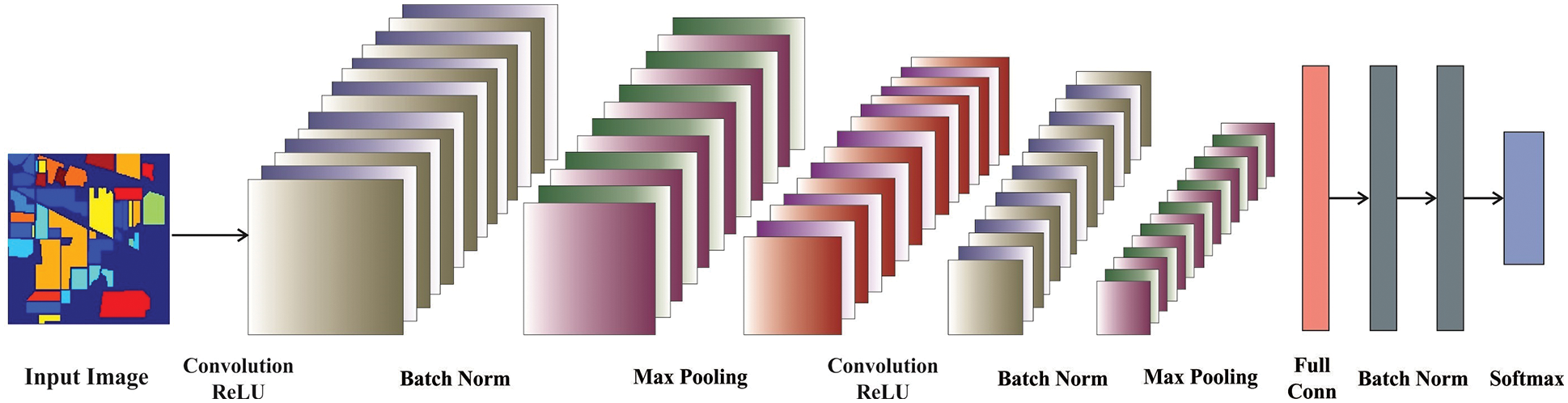
Figure 1: Structure of CNN

There are 4 blocks from the decoded. All the blocks start with up-sampling that is expand the feature map, then convolutional and rectified linear unit (ReLU). The batch normalization layer is then executed for all of the maps. The primary decoder that is nearby the final encoded is generate a multi-channel feature map. It can be related to Segnet that it creates a distinct amount of sizes and channels as its encoded input. The last output of final decoder layer was able to a trainable softmax classification that generates a K channel image of probability in which K is the amount of class labels. The forecasted segmentation equals the class with maximal probability at all the pixels.

For tuning the hyperparameters that exist in the NasNet model, the Adagrad optimizer is applied. Adagrad is a technique to gradient-based optimized that adjusts the rate of learning to the parameters. Adagrad enhanced significantly and it can be utilized to train large scale neural network (NNs) at Google. Besides, it is utilized Adagrad for training Word Embedded. It can be utilized for setting gradient of object function was represented by gi,j , in terms of parameter θi at timestep t.

gt,i=∇θJ(θ) (1)

The SGD upgrade to all the parameters θi at all the timestep t then develops:

θt+1,i=θi,j−α.gt,i (2)

Their update rule, Adagrad changes the common rate of learning at all the timesteps t to all the parameters θi dependent upon the past gradient which is calculated for θi :

θt+1,i=θi,j−αGt,ii+ϵ.gt,i (3)

Gt∈Rd×d at this time is a diagonal matrix in which all diagonal elements i, i refers the sum of squares of the gradients in terms of θi up to timestep t , but ϵ refers the smoothing term which avoids division by zero. The default value of the rate of learning for Adagrad is 0.01. The structure of GRU model is depicted in Fig. 2.

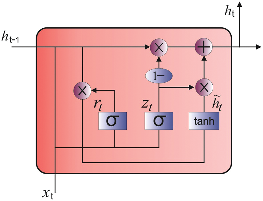
Figure 2: GRU model

2.2 HS Image Classification

For HS image classification, the GRU model is employed which determines the class labels efficiently [17]. In GRU, the two vectors in long short term memory (LSTM) cells are associated with one vector ot . One gate controller controls the integrated form of forgetting and input gates. When zt output is one, the forget gate was opened, and input gate was closed, when zt was zero, the forget gate was closed, and the input gate was opened. Instinctively, the reset gate determines by integrating an input with previous memory, and the upgrade gate elects the prior memory information has preserved to estimate the new state. The variance in the LSTM, however the variations formerly determined by:

rt=σ(WxrT⋅xt+WorT⋅ot−1+br). (4)

zt=σ(WxzT⋅xt+WoTz⋅ot−1+bz). (5)

o~t=tanh(Wxo~T⋅xt+Woo~T⋅(rt⊗ot−1)+bo~). (6)

ot=zt⊗ot−1+(1−zt)⊗ot. (7)

whereas Wxr,Wxz,Wxo~ denotes weight matrices to corresponding input vector, Wor,Woz,Wo denotes the weight matrices of prior time step, and br,bz,bo~ represent bias.

2.3 Parameter Optimization

In order to effectually determine the parameters involved in the GRU model, the RDA is exploited [18]. RDA is analogous to other meta-heuristics, initiated by an arbitrary population viz. red deer (RD) counterpart. An optimal RD from the population is carefully chosen and named the “male RD (MRD)”, then the residue was called “hinds” [18]. The iteration presentation of method was coined. To arithmetical process the RDA initiates by Eq. (8) while a key population to the RD is created:

RD=X1,X2,X3,…,XNvar (8)

Next, the fitness of each member from the population is calculated as follows:

Value=f(RD)=f(X1,X2,X3,…,XNvar) (9)

MRD is try to boost the grace by roaring in this phase. Therefore, the outcomes, the roaring method could fail or succeed. Once the key functions of neighbor are MRD, it is replaced with the prediction once it is larger than the previous MRD. The succeeding formula is shown below:

malenew={maleold+a1(UB−LB)*a2+LB), if a3≥0.5maleold−a1(UB−LB)*a2+LB), if a3<0.5  is less than 0 (10)

UB and LB bounds the searching region to create apt male neighborhood solution. The top and lower limits of searching region. Clear the present location of MRD is maleold , and the following location is malenew . The sum of male commanders is estimated by the following:

Nc=round(γ.Nmale) (11)

whereas NC denotes the sum of commanders that naturally males, γ indicates the arbitrary amount among [0,1] Nmale characterizes the sum of whole males. It is noted that γ denotes the method initials value. It is value ranges within [0,1]. Eventually, the sum of stags is assessed by the succeeding formula:

Ns=Nmale−Nc (12)

The fighting method can be modelled by the following 2 arithmetical formulas:

new1=C+S2+b1((UB−LB)∗b2+LB) (13)

The subsequent equation is employed to calculate commander standardization power.

Pn=|Vn∑i=1ai⁡Vi| (14)

The sum total of hinds of a harem is calculated by:

N.haremn=round(Pn⋅Nhind) (15)

whereas Nhind denotes the complete quantity of hinds. It could be deer mating presentation was executed by commander with proportion of hinds from their harem.

N.haremnmate=round(α⋅N.haremn) (16)

The sum total of hinds from the nth harem that mate with leader represent N.haremnmate . Regarding the solution space, it selects N.haremnmate of N.haremk arbitrarily. In general, the mating technique has described in the following:

offs=C+Hind2+(UB−LB)×c (17)

It chooses a harem arbitrarily (k) and permits the male commander to mate with β percentage of harem hinds. The quantity of hinds from the harem that mate with commander is estimated by the succeeding formula:

N.haremkmate=round(β⋅N.haremk) (18)

whereas N.haremkmate denotes the quantity of hinds from the kth harem that mate with commander. It is noted that the mating procedure was implemented by Eq. (17). Fig. 3 depicts the process involved in RDA. The distance among a stag and hind from J dimension space is estimated by [19]:

di={∑j˙eJ⁡(stagj˙−hindj˙i)2}12 (19)

Now di denotes the distance among the ith hind and stag.

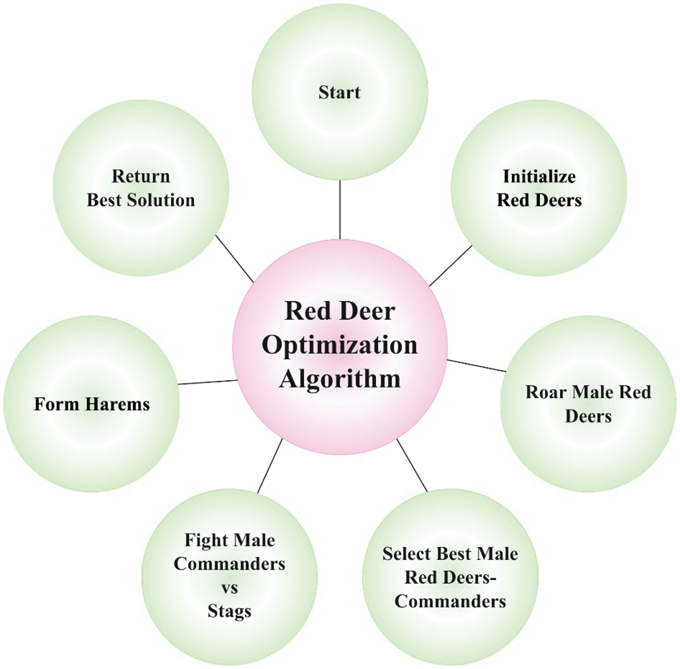
Figure 3: Process involved in RDA

3  Results Analysis

The performance validation of the RDADL-HIC model is examined using Indian Pines dataset (IPD) and Pavia university dataset (PUD), available at http://www.ehu.eus/ccwintco/index.php/HS_Remote_Sensing_Scenes. The first IPD includes 10249 data instances under 16 class labels. The second PUD encompasses 42776 data instances with 9 class labels.

Fig. 4 demonstrates the training accuracy (TA) and validation accuracy (VA) offered by the RDADL-HIC model on IPD. The figure indicated that the RDADL-HIC model has provided closer TA and VA values with an increase in epoch count. It is observable that the VA is certainly higher than TA. Fig. 5 validates the training loss (TL) and validation loss (VL) provided by the RDADL-HIC model on IPD. The figure designated that the RDADL-HIC model has delivered lower TL and VL with an increase in epoch count. It is noticeable that the VL is definitely lower compared to TL.

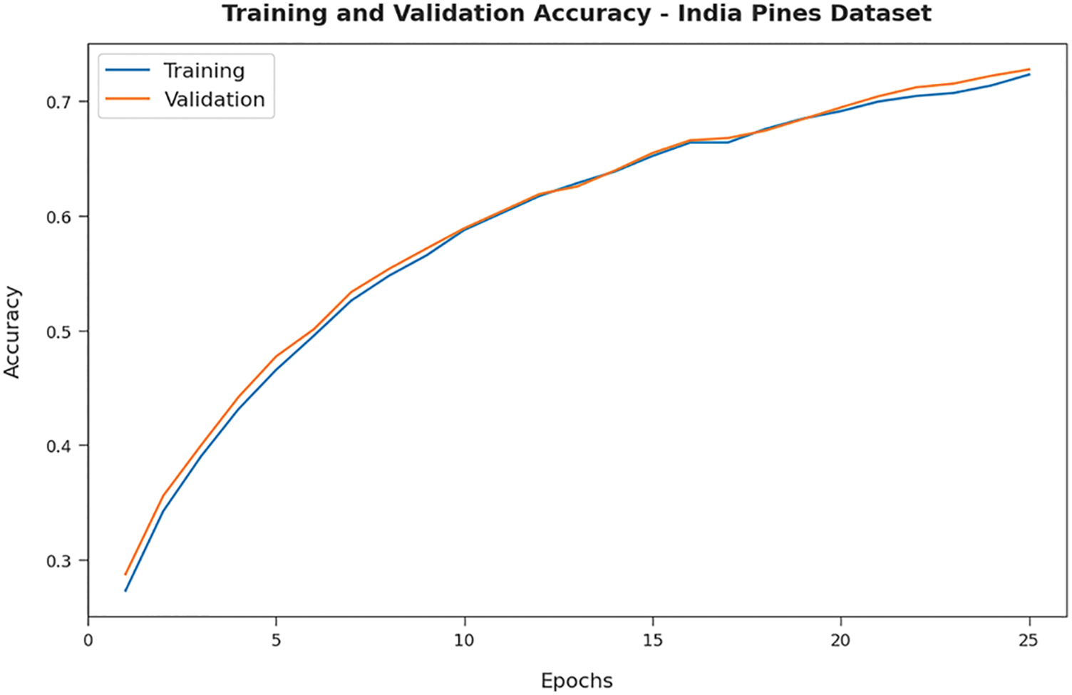
Figure 4: TA and VA of RDADL-HIC model on IPD

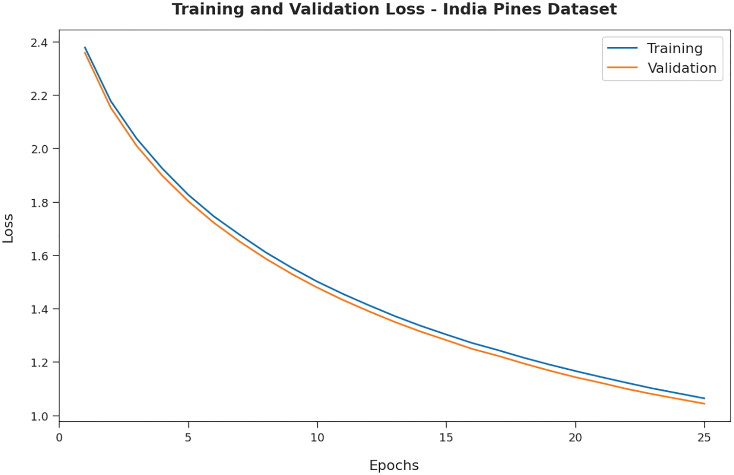
Figure 5: TL and VL of RDADL-HIC model on IPD

Fig. 6 illustrates the precision-recall investigation of the RDADL-HIC model on the IPD. The figure indicated that the RDADL-HIC model has accomplished maximum precision-recall values on the distinct class labels.

Fig. 7 exemplifies the ROC assessment of the RDADL-HIC model on the IPD. The figure indicated that the RDADL-HIC model has gained improved ROC values on the distinct class labels.

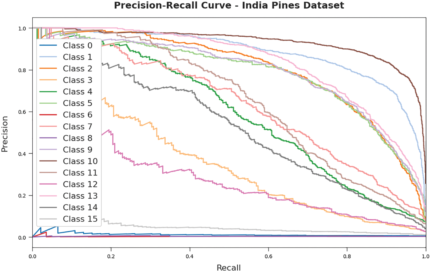
Figure 6: Precision-recall curves of RDADL-HIC model on IPD

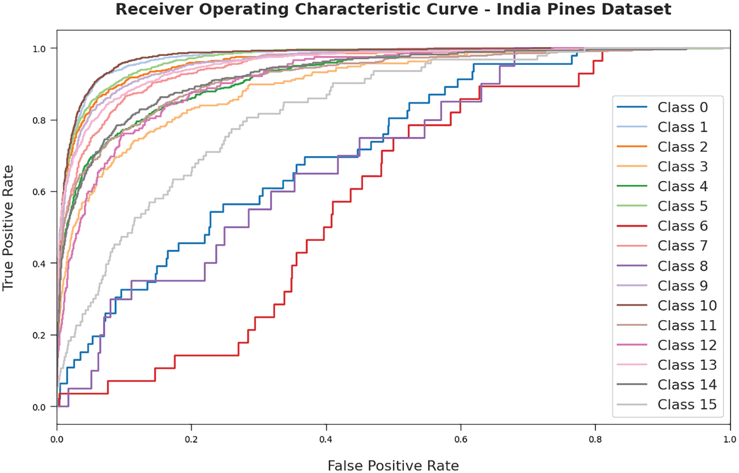
Figure 7: ROC curves of RDADL-HIC model on IPD

Next, the experimental validation of the RDADL-HIC model is tested using PUD. Fig. 8 illustrates the sample input image with its ground truth version. Fig. 9 proves the TA and VA obtainable by the RDADL-HIC model on PUD. The figure indicated that the RDADL-HIC model has provided closer TA and VA values with an increase in epoch count. It is observable that the VA is certainly higher than TA.

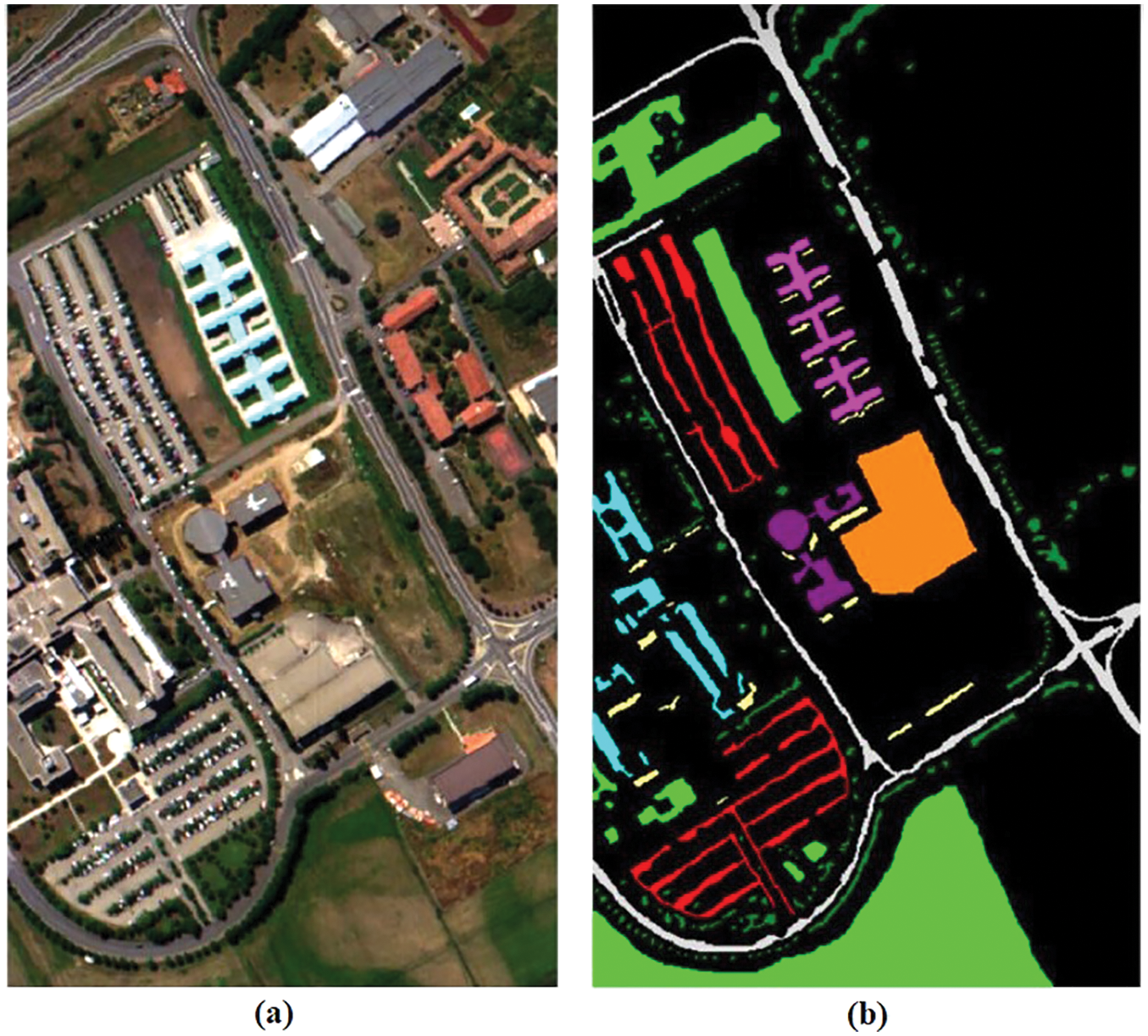
Figure 8: PUD. (a) Sample Image, (b) Ground Truth

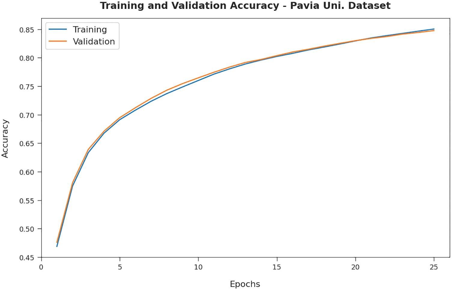
Figure 9: TA and VA of RDADL-HIC model on PUD

Fig. 10 confirms the TL and VL delivered by the RDADL-HIC model on PUD. The figure designated that the RDADL-HIC model has delivered lower TL and VL with an increase in epoch count. It is noticeable that the VL is definitely lower compared to TL.

Fig. 11 illustrates the precision-recall study of the RDADL-HIC model on the PUD. The figure indicated that the RDADL-HIC model has accomplished maximum precision-recall values on the distinct class labels.

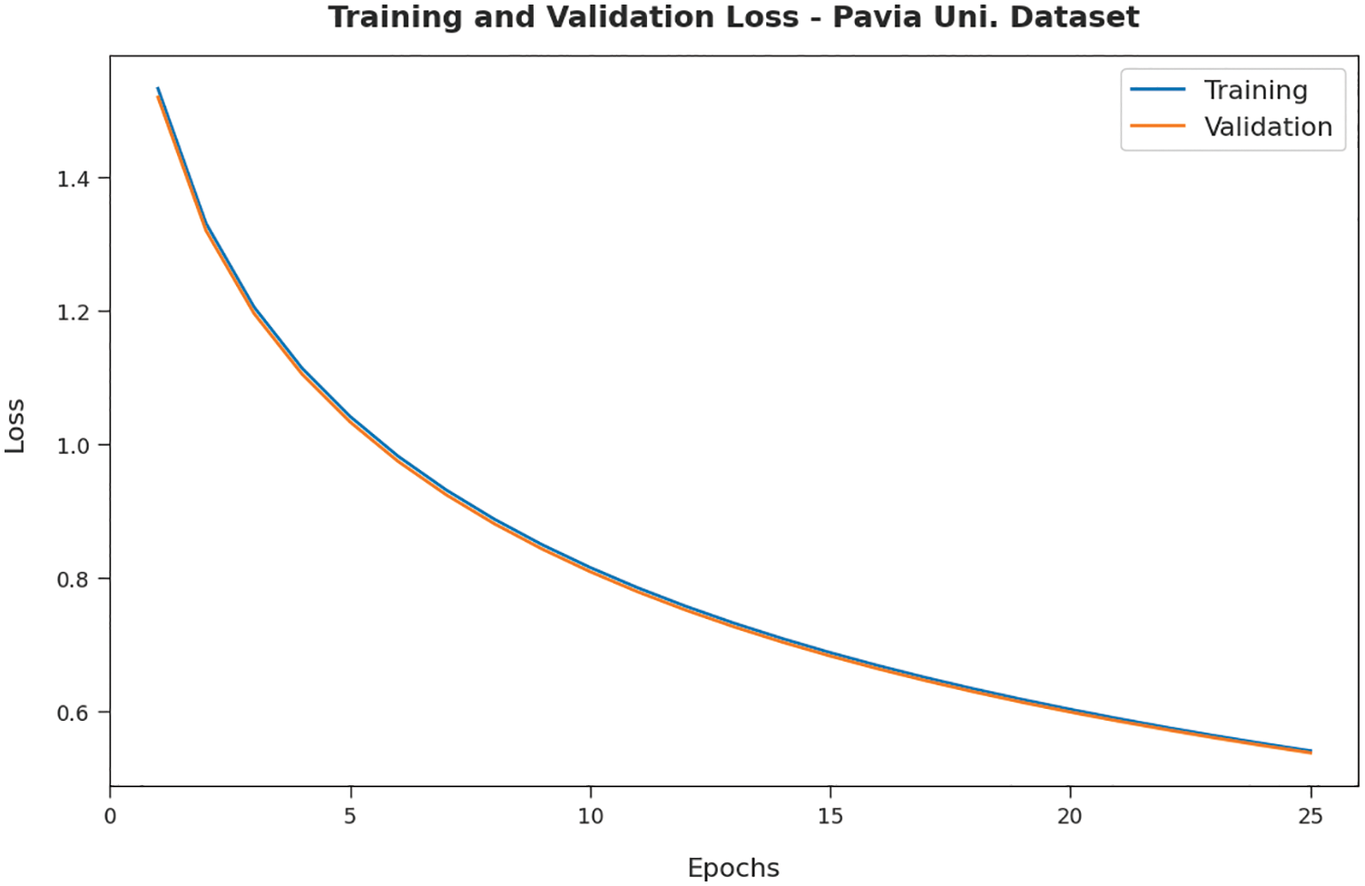
Figure 10: TL and VL of RDADL-HIC model on PUD

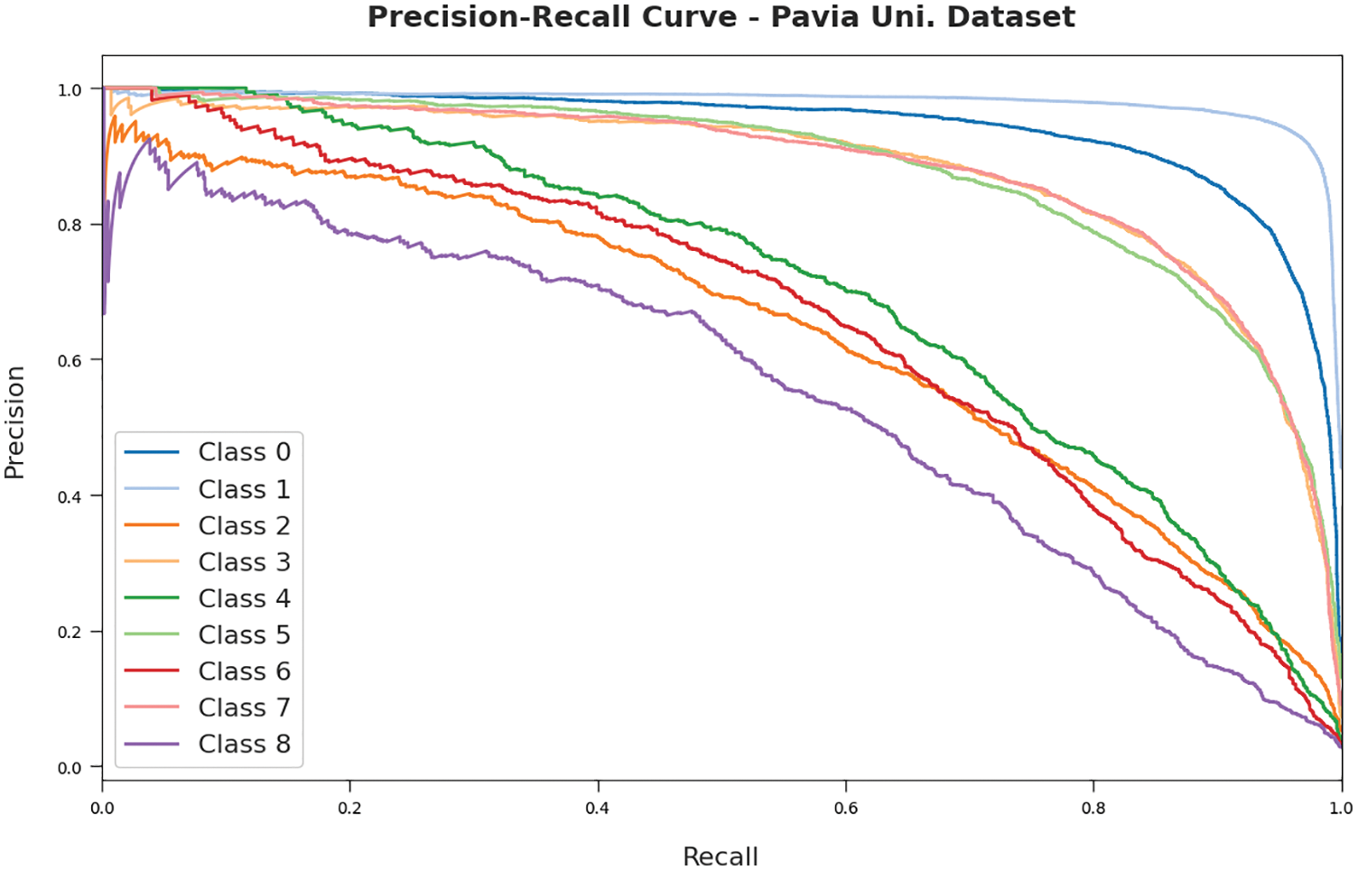
Figure 11: Precision recall curves of RDADL-HIC model on PUD

Fig. 12 exemplifies the ROC assessment of the RDADL-HIC model on the PUD. The figure indicated that the RDADL-HIC model has gained improved ROC values on the distinct class labels. For ensuring the enhanced outcomes of the RDADL-HIC model, a detailed comparative examination with IPD and PUD datasets is made in Tab. 1 [20,21].

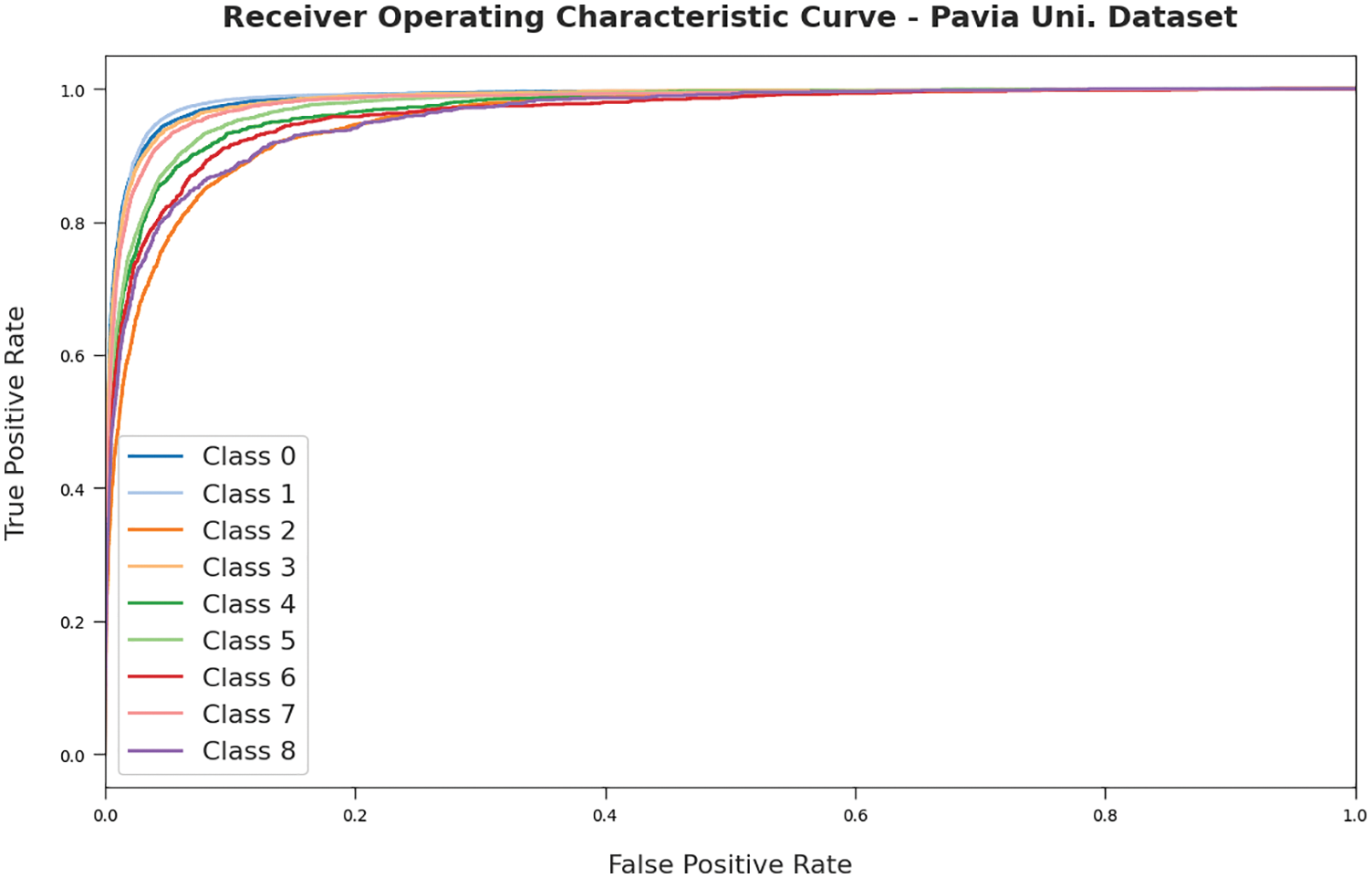
Figure 12: ROC curves of RDADL-HIC model on PUD

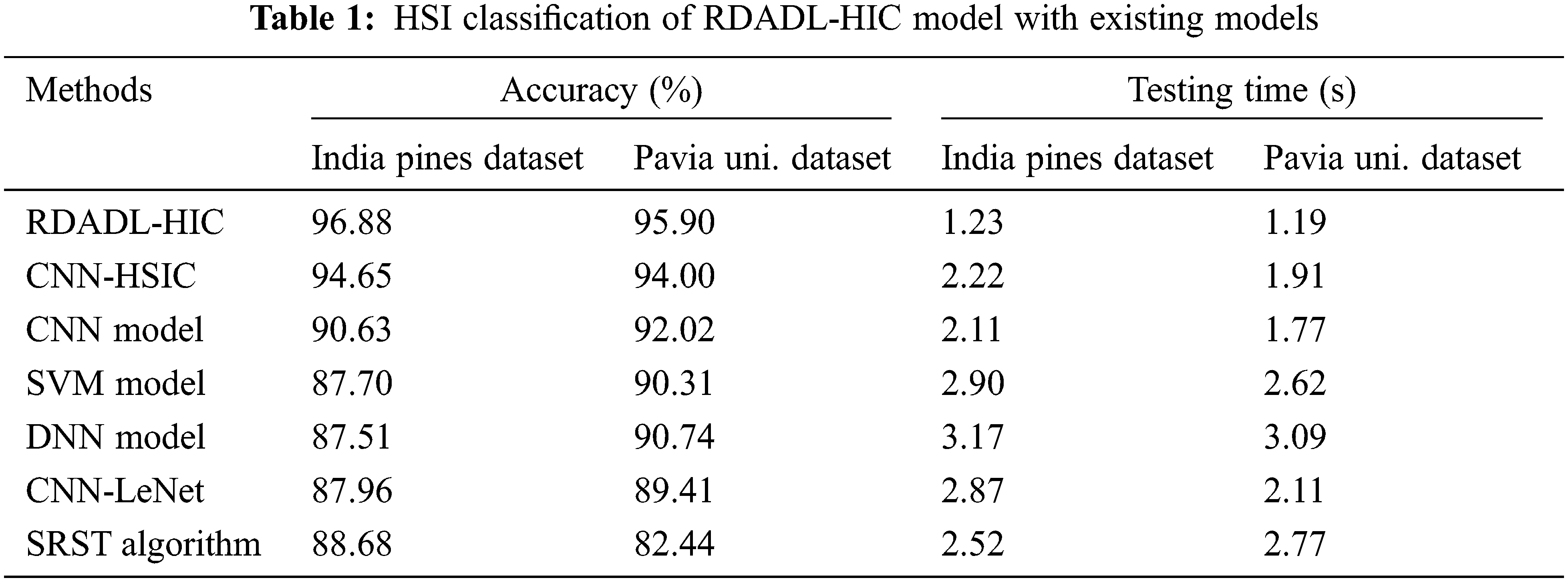
Fig. 13 demonstrates a brief accuracy examination of the RDADL-HIC model with existing models on IPD and PUD. The figure indicated that the support vector machine (SVM), deep neural network (DNN), CNN-LeNet models have shown poor outcomes with minimal values of accuracy. Though the CNN-HSIC and CNN models have attained moderate accuracy values, the presented RDADL-HIC model has accomplished maximum accuracy on both datasets. For instance, on IPD, the RDADL-HIC model has attained higher accuracy of 96.88% whereas the CNN-HSIC, CNN, SVM, DNN, CNN-LeNet, and SRST models have obtained lower accuracy of 94.65%, 90.63%, 87.70%, 87.51%, 87.96%, and 88.68% respectively. Similarly, on PUD, the RDADL-HIC model has reached increased accuracy of 95.90% whereas the CNN-HSIC, CNN, SVM, DNN, CNN-LeNet, and SRST models have gotten reduced accuracy of 94%, 92.02%, 90.31%, 90.74%, 89.41%, and 82.44% respectively.

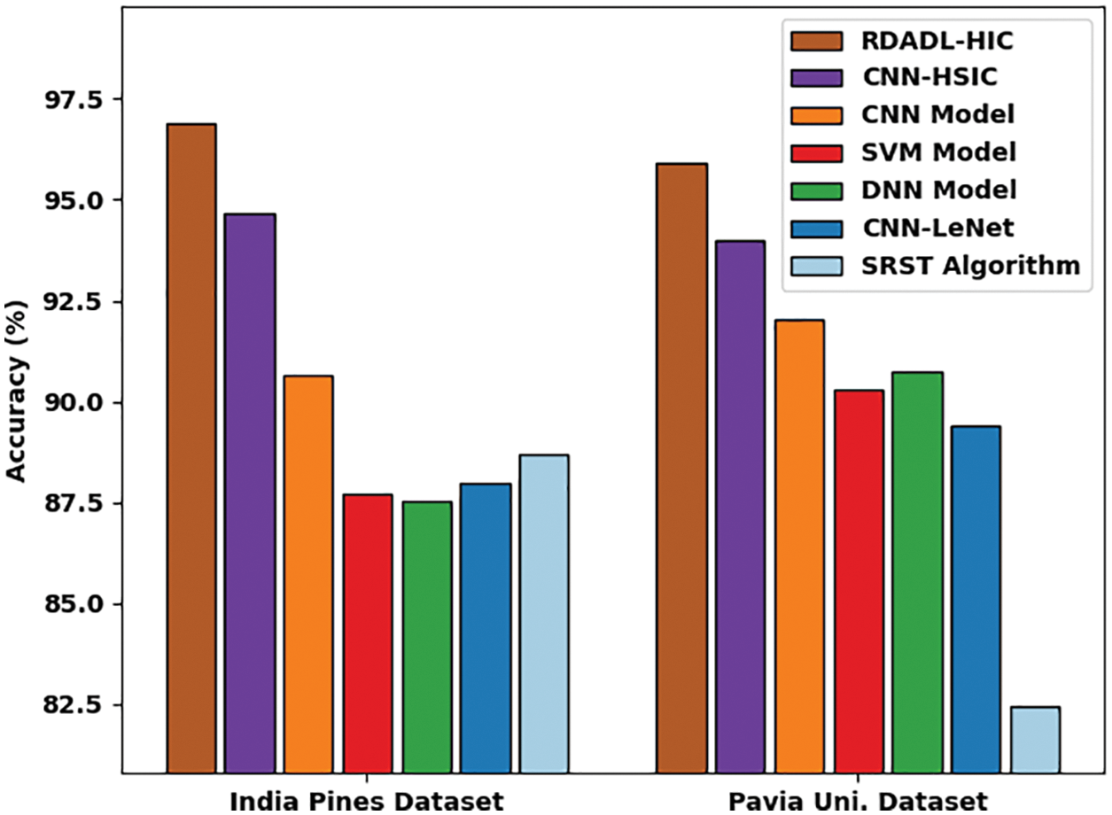
Figure 13: Comparative accuracy analysis of RDADL-HIC model with existing models

Fig. 14 exhibits a detailed testing time (TT) inspection of the RDADL-HIC model with recent approaches on IPD and PUD. The results represented that the SVM, DNN, CNN-LeNet models have exposed worse performance with maximum values of TT. Although the CNN-HSIC and CNN models have attained reasonable TT values, the presented RDADL-HIC model has gained lower values of TT on both datasets. For instance, on IPD, the RDADL-HIC model has accomplished reduced TT of 1.23 s whereas the CNN-HSIC, CNN, SVM, DNN, CNN-LeNet, and SRST models have attained increased TT of 2.22 s, 2.11 s, 2.90 s, 3.17s, 2.87 s, and 2.52 s respectively.

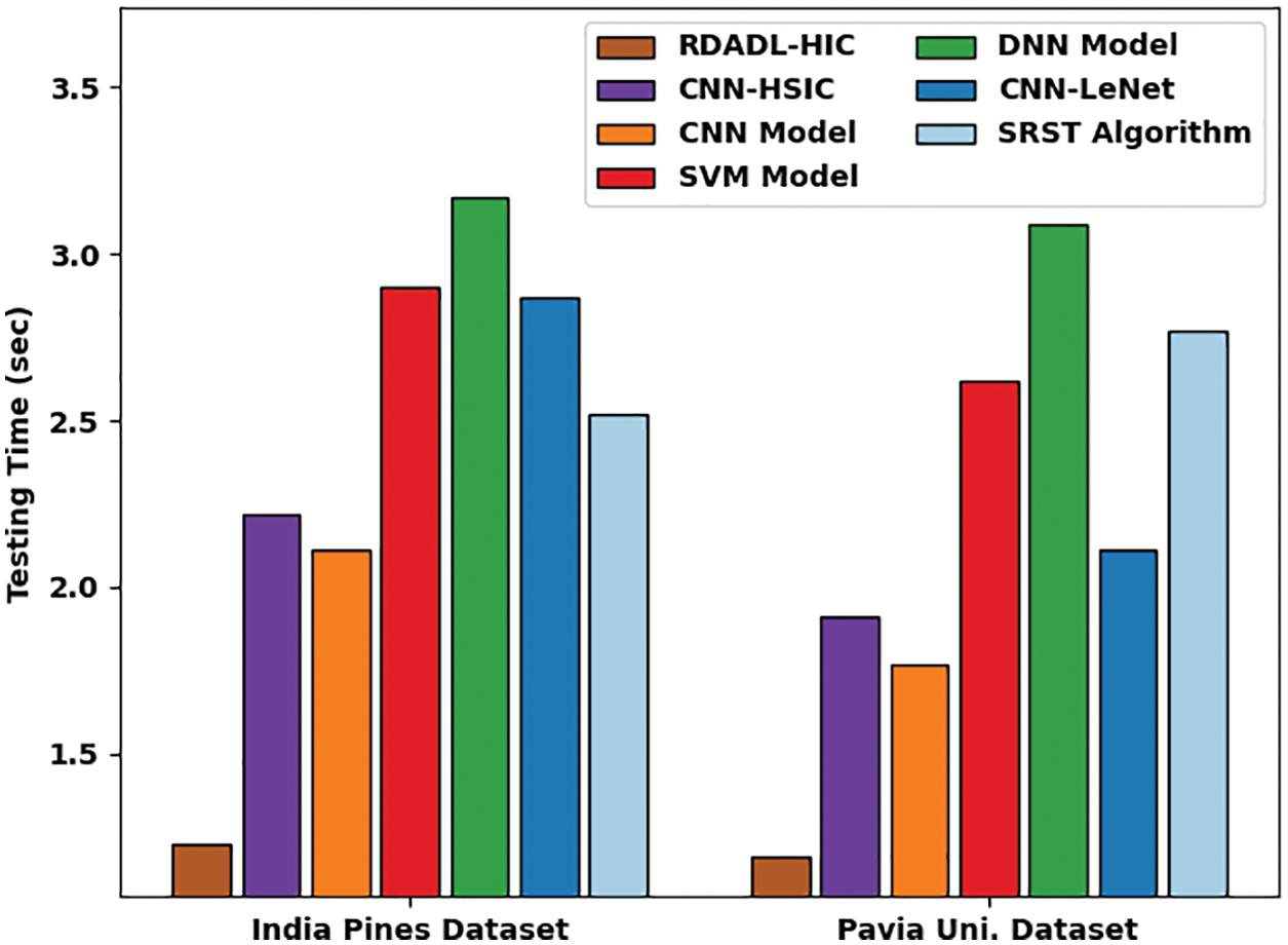
Figure 14: Comparative TT analysis of RDADL-HIC model with existing models

Likewise, on PUD, the RDADL-HIC model has obtained lower TT of 1.19s whereas the CNN-HSIC, CNN, SVM, DNN, CNN-LeNet, and SRST models have gotten reduced TT of 94%, 1.91 s, 1.77 s, 2.62 s, 3.09 s, and 2.11 s respectively. When the results and discussions are observed, it is concluded that the RDADL-HIC model has accomplished maximum performance on HS image classification.

4  Conclusion

In this study, a novel RDADL-HIC technique has been presented to effectively determine the HSI images. The RDADL-HIC technique mainly involves a NASNetLarge model with Adagrad optimizer. Followed by, RDA with GRU classifier is used for the identification and classification of HSIs. The design of Adagrad optimizer with RDA helps to automatically modify the hyperparameters of the NASNetLarge and GRU models respectively. The experimental results stated the superior results of the RDADL-HIC model and the results are inspected interms of different measures. The comparison study of the RDADL-HIC model demonstrated the enhanced performance over its recent approaches. In future, the proposed model can be employed in real time application such as agriculture, mineral exploration, etc.

Funding Statement: The authors received no specific funding for this study.

Conflicts of Interest: The authors declare that they have no conflicts of interest to report regarding the present study.

This work is licensed under a Creative Commons Attribution 4.0 International License, which permits unrestricted use, distribution, and reproduction in any medium, provided the original work is properly cited.