@Article{icces.2023.010519,
AUTHOR = {Xiaoyang Shen, Xiaojing Zhang},
TITLE = {Damage Identification Algorithm of Composite Structure Based on Displacement Field},
JOURNAL = {The International Conference on Computational \& Experimental Engineering and Sciences},
VOLUME = {28},
YEAR = {2023},
NUMBER = {1},
PAGES = {1--3},
URL = {http://www.techscience.com/icces/v28n1/55228},
ISSN = {1933-2815},
ABSTRACT = {1 General Introduction
Reliable structural health monitoring with high detection probability is very important [1]. Therefore,
the method of finite element simulation was adopted. Based on the basic equation of material mechanics
and stiffness degradation theory, to detect the damage of composite laminates, and further improves the
intelligence of the detection process through the method of visual detection neural network.
2 Theoretical derivation and simulation
2.1 Equations for buckling
In the stratified damage area, each layer bears the load independently, and the bearing capacity is
determined by the stiffness there: the larger the axial stiffness, the stronger the bearing capacity at the
stratified area. [2] The higher the bending stiffness, the greater the critical buckling load.
When the layer with lower bending stiffness reaches the buckling load, the layer will no longer bear the load,
and the load will continue to be borne by the damage site with higher stiffness.[3] When the layer with the
maximum stiffness also reaches the buckling load, local buckling will occur in each layer of the sub-plate at
the same time.
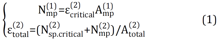
Based on this conclusion, the load can be calculated using the known stiffness of the substrate Amp
(1) and
the critical strain of another substrate  .
.
 .
.
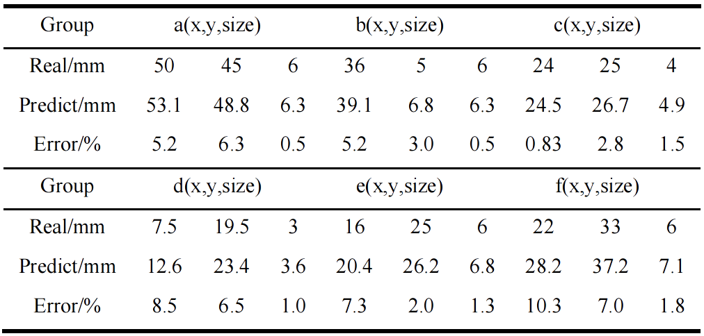
Compared the predicted parameters with the actual parameters, the results are shown in Table 2. The
average relative error of the neural network model for coordinate prediction is 5.41%, and the prediction
effect is good, which is larger than the actual value, which proves that there is still room for adjustment. The
average relative error of the model for predicting the damage size is 1.1%, and the prediction effect is quite
in line with the expectation.
2.2 Preparation for simulation
The size of the model selected in this work is 60mm×60mm, and the layup of the laminate is [0°/45°/-
45°/90°]s. Compression load of 1mm was loaded to make the laminates deform in the direction out of plane.
In order to simulate the interlayer force in Abaqus, a cohesive force unit with a thickness of 0 is biased
between adjacent layers, and the interlayer damage simulated by the stiffness reduction method is shown
in Table.1.
2.3 Database of the simulation
On the basis of parameterized modeling using Python, 700 groups of models containing damage were
established through for loop which randomly assigns the size and location of damage through random
function. The damage radius is controlled within 2-8mm, and the damage may occur at any interlayer
position.
3 Analysis and algorithm
3.1 Analysis of database
The cloud image is derived as shown in Figure.1. The color difference in the cloud image can better
reflect the damage appearance of the laminates. It should be noted that different cloud images need to unify
the color range in Abaqus software. From the photo gallery, it can be roughly seen that the colors of different
pictures are relatively uniform, and there are no obvious inappropriate samples.
3.2 Image processing
During the image processing, the non-maximum suppression algorithm was used to select the box with
the highest evaluation and suppress the box with the lower evaluation. This process is an iterative
elimination process shown in Figure.2.
4 Conclusion
Figure.3 shows the relationship curve between accuracy and recall of the model. The average accuracy
of this model is 0.89. If the 45° reference line is taken as the equilibrium point of P=R, it can be found that
the equilibrium point of this model is very high, indicating that the algorithm is suitable for this work.
Table 1: Cloud image of displacement field
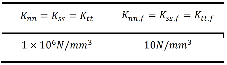
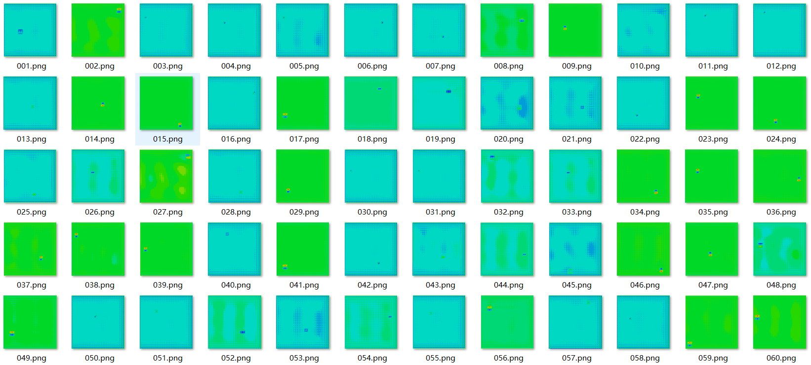
Figure 1: Cloud image of displacement field
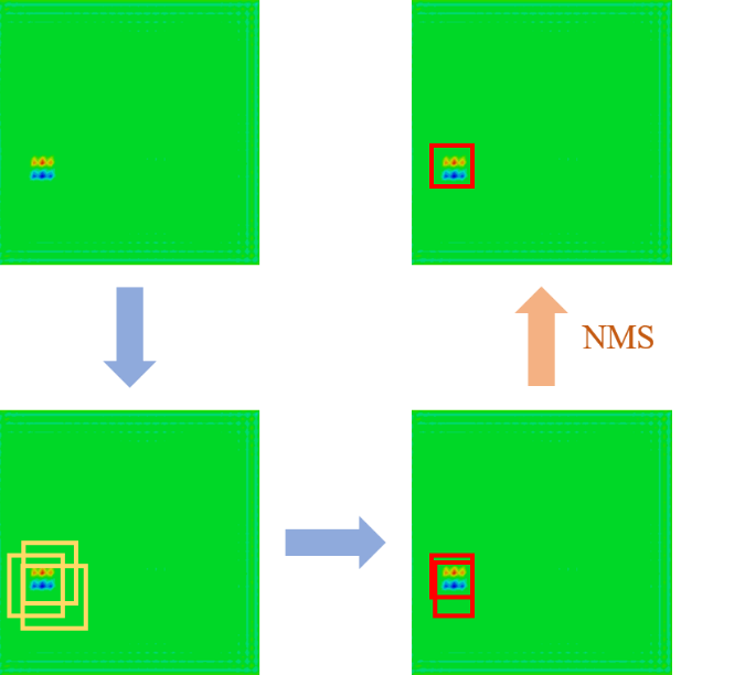
Figure 2: Non-maximum suppression algorithm
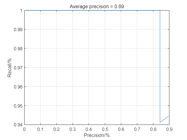
Figure 3: Cloud image of displacement field
Table.2: Predicted parameters and errors
 },
DOI = {10.32604/icces.2023.010519}
}
},
DOI = {10.32604/icces.2023.010519}
}