Journal of Quantum Computing DOI:10.32604/jqc.2022.026975
Article

Research on Rainfall Estimation Based on Improved Kalman Filter Algorithm

Wen Zhang1,2, Wei Fang1,3,*, Xuelei Jia1,2 and Victor S. Sheng4

1Engineering Research Center of Digital Forensics, Ministry of Education, School of Computer & Software, Nanjing University of Information Science & Technology, China
2Nanjing Xinda Institute of Meteorological Science and Technology Co., Ltd., Nanjing, 210044, Jiangsu, China
3State Key Laboratory of Severe Weather, Chinese Academy of Meteorological Sciences, China
4Department of Computer, Texas Tech University, Lubbock, TX 79409, USA
*Corresponding Author: Wei Fang. Email: Fangwei@nuist.edu.cn
Received: 09 January 2022; Accepted: 29 April 2022

Abstract: In order to solve the rainfall estimation error caused by various noise factors such as clutter, super refraction, and raindrops during the detection process of Doppler weather radar. This paper proposes to improve the rainfall estimation model of radar combined with rain gauge which calibrated by common Kalman filter. After data preprocessing, the radar data should be classified according to the precipitation intensity. And then, they are respectively substituted into the improved filter for calibration. The state noise variance Q(k) and the measurement noise variance R(k) can be adaptively calculated and updated according to the input observation data during this process. Then the optimal parameter value of each type of precipitation intensity can be obtained. The state noise variance Q(k) and the measurement noise variance R(k) could be assigned optimal values when filtering the remaining data. This rainfall estimation based on semi-adaptive Kalman filter calibration not only improves the accuracy of rainfall estimation, but also greatly reduces the amount of calculation. It avoids errors caused by repeated calculations, and improves the efficiency of the rainfall estimation at the same time.

Keywords: Kalman filter; doppler radar; rainfall estimation; radar-rain gauge joint calibration

1  Introduction

In recent years, various industries in our country have highly affirmed the economic and social values contained in meteorological data. Meteorological early warning and forecasting play a vital role in the development of all walks of life in our country. With the innovation and development of meteorological technology, the requirements of meteorological users for weather forecasting and early warning products are also increasing [1].

With the continuous improvement of remote sensing technology, the use of radar to complete meteorological work has become one of the more common and respected methods nowadays. The echo pictures, data, charts and other information of weather phenomena obtained by Doppler radar detection provide important data basis for short-term or very short-term weather forecasts of meteorological forecasting and early warning research departments. It is a very good tool for sexual weather inspection, forecasting and early warning [2].

However, the meteorological data information obtained in actual measurement is often mixed with other noises. If you want to obtain accurate weather forecasts from the data with noise interference, you need to eliminate useless noise interference as much as possible [3]. The weather forecast made directly based on the Doppler radar observation data is actually a series of forecast value time series with errors. They are still far from the accuracy of actual weather. The Kalman filter algorithm is an important method to process this kind of forecast data with errors to get the best estimate, thereby improving the accuracy of the forecast [4].

So far, Kalman filter has been well applied in the field of meteorological business and has achieved certain success. In 2004, Zheng et al. [5] used Kalman filter calibration method, probability matching method and optimization method to estimate precipitation in different climatic regions in the rainy season of the Huai River Basin, and found that the Kalman filter calibration method has the best rainfall estimation effect. In 2005, Zhao et al. [6] used an adaptive Kalman filter method to forecast a flood process, and found that the calibrated forecast result is closer to the actual value. In 2005, Yin et al. [7] used the Kalman filter calibration method to improve the accuracy of radar quantitatively estimate of regional precipitation, and found that the accuracy of the calibration method for estimating precipitation will increase with the increase of the number of observations. In 2012, Dong et al. [8] passed the precipitation data of three different types of precipitation weather processes in Tianjin according to the analysis, it was concluded that the result of radar-rain gauge joint calibration rainfall estimation will be more accurate as the density of the rain gauge increases. In 2019, Wang et al. [9] proposed the weighted integration of SVM and Kalman, which obtained the stability and accuracy of temperature forecast calibration in mountainous scenic spots have been improved.

2  Related Work

2.1 Radar Rainfall Estimation

The Doppler radar measurement obtains the radar reflectivity factor Z that effectively illuminates the precipitation particles in the body. Its value is directly related to the droplet spectrum, and the droplet spectrum directly determines the precipitation intensity I, which means that there is also a certain correlation between the radar reflectivity factor Z and the precipitation intensity I [10].

Precipitation depends on the geometry, number density, and phase state of the precipitation particles within the detection range. The intensity of precipitation depends on the number density and the final velocity of the precipitation particles. The geometry and form of the precipitation particles directly affect the falling speed of precipitation particles. Therefore, the principle of Doppler weather radar forecasting precipitation is to measure the intensity of precipitation I in the relevant area or a single point through the echo intensity Z received by the Doppler radar.

The relationship between Z-I is shown in the following formula (1):

Z=AIb(1)

In formula (1), I represents the mass of water falling on the cross-sectional area of unit area per unit time, the unit is mm/h. Z represents the radar reflectivity factor, the unit is mm6/m3. The coefficients A and b are determined by the measured data, and are often substituted into the values which meet certain accuracy requirements. Their specific values are related to the geographic conditions and specific precipitation types of each study area, and can be adjusted accordingly.

However, due to the distribution of raindrop spectrum is different for different precipitation types and different regions, the coefficients A and b also have large changes. In addition, because the method of using the Z-I relationship to estimate the precipitation completely relies on the radar reflectivity factor Z measured by the Doppler radar, and various external factors such as the height and distance measured by the radar lead to the Z cannot be able to fully objectively reflect the actual precipitation situation. Therefore, we can conclude that although the method of realizing rainfall estimation through the Z-I relationship is simple and easy, the accuracy of the rainfall estimation is not high.

In order to solve the problem that the radar rainfall estimation accuracy obtained by the Z-I relation method is not high. Somebody proposed to calibrate it. At present, the methods to calibrate Doppler weather radar rainfall estimation are mainly divided into two categories. The first category is calibration without a rain gauge, which is mainly to calibrate the coefficients A and b according to the above-mentioned Z-I relationship to obtain the best coefficient value. The second category is calibration with rain gauges. This method of real-time calibration using rain gauges includes single-point calibration, average calibration, distance-weighted calibration and Kalman filter calibration, etc. This method makes up for the deficiency that the precipitation intensity obtained by using Doppler weather radar alone is affected by the uncertainty of the Z-I relationship and radar parameters.

In the study of rainfall estimation using Doppler weather radar combined with rain gauge, it is usually necessary to select a set of values of A and b based on experience. Normally, the Z-I relationship is set to [11]:

Z=200I1.6(2)

The precipitation rate can be calculated according to the Z-I relationship. And the initial value field is reversed. We can obtain the calibration factor f from the rain gauge data of the automatic weather station. The product of the calibration factor f and the initial value field is used as the final rainfall estimate.

2.2 Automatic Weather Station

The establishment of automatic weather stations can help people better and more accurately grasp the changes of weather. They can automatically detect multiple elements according to the needs of a certain area without manual intervention, and automatically generate messages to transmit the detected data to the central station regularly [12].

The establishment of automatic weather stations provides data in places that are difficult for people to access or are not suitable for living, enhances the density of the observation station network and can provide some measurement data outside the normal manual measurement time. What's more, automatic weather stations can effectively increase the reliability of observation data by new technologies. Compared with manual measurement, it can effectively reduce human error. To a large extent, the consumption and expenditure of human resources for measuring data are reduced.

At present, the construction of automatic weather stations around the world has been very extensive and mature. Corresponding weather stations are also set up in various regions of our country. As shown in Fig. 1 below, the orange circles in the figure show the distribution of some weather stations around the world, and the yellow circles correspond to the distribution of automatic weather stations in our country. From the figure, we can see that the establishment of automatic weather stations in our country is relatively intensive.

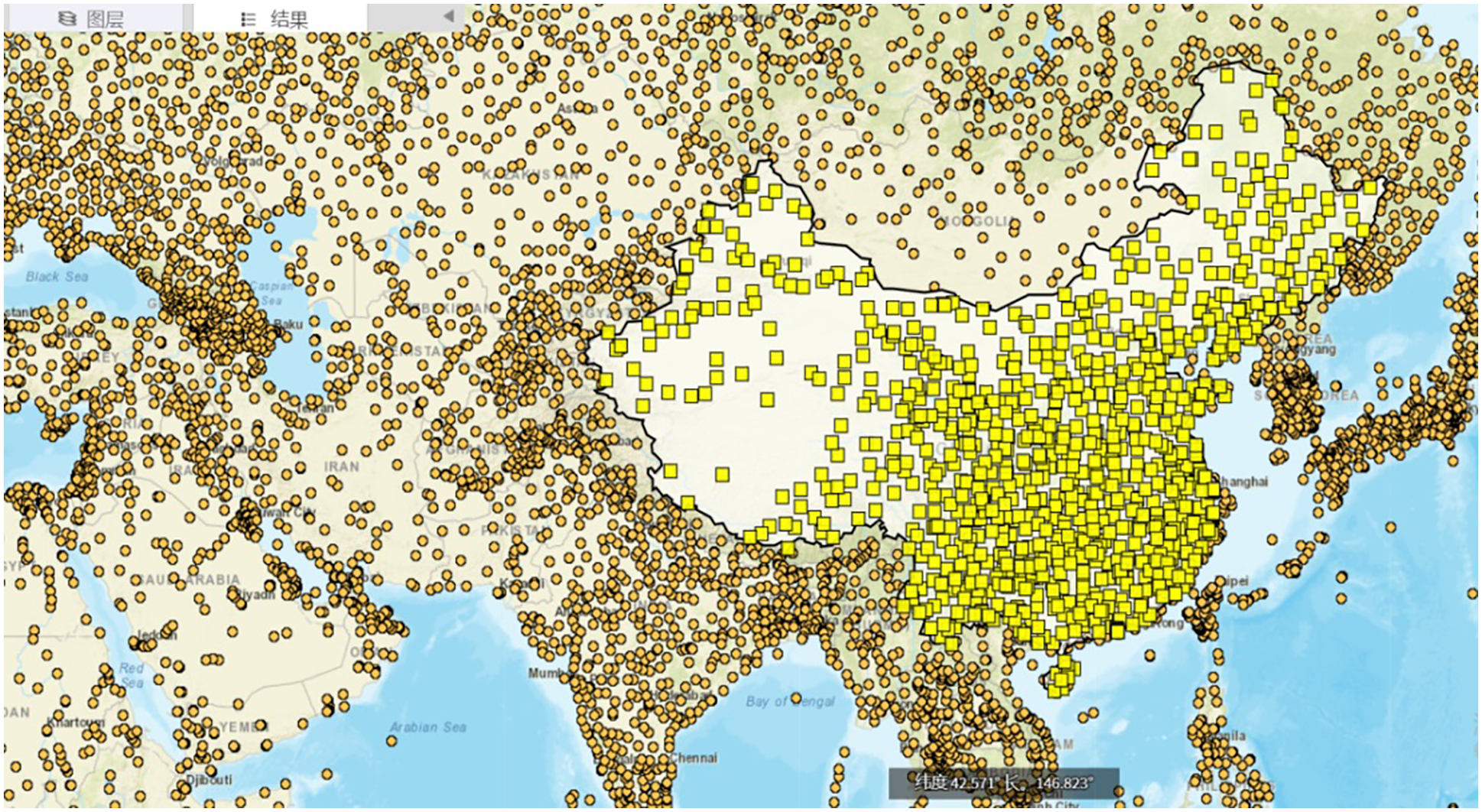
Figure 1: Distribution map of automatic weather stations

2.3 Kalman Filter Algorithm

Kalman Filtering is an estimation method first proposed by the mathematician R.E.Kalman for the problem of stochastic process state estimation [13]. The Kalman filter algorithm is essentially a time-domain recursive algorithm, with the minimum mean square error as the best estimation criterion. It can estimate the current state based on the estimated value of the previous state and the observed value of the current state. This is also a significant feature of the Kalman filter algorithm. It does not need to store a large amount of historical data, so it is convenient for computer implementation.

So far, Kalman filter has been widely used in robot navigation, target tracking, signal processing, aerospace and other fields. In the rainfall estimation, Kalman filtering is also an effective means to eliminate random interference and improve the accuracy of weather forecasting [14].

The Kalman filter algorithm defines the state variable as X and the observation variable as Z. The state of the system is as follows (3):

Xk=AXk−1+Buk−1+ωk−1(3)

The state equation is to infer the current state based on the state and control variables at the previous moment, where A which is an n∗n-order square matrix represents the state transition matrix. It is the basis for predicting state variables. uk−1 represents the control gain at time k − 1. In most cases, this variable is set to 0. ωk−1 is considered to be the prediction process noise that obeys the Gaussian distribution. It corresponds to the noise of each component in Xk. It is Gaussian white noise with expectation of 0 and covariance of Q. ωk∼N(0,Q).Q corresponds to the process excitation noise Q appearing below.

The Kalman filter observation equation is as formula (4):

Zk=HXk+vk(4)

vk represents the measurement noise. Like the above-mentioned prediction process noise, it is defaulted to be mutually independent and normally distributed white noise in the application of the Kalman filter algorithm, which obeys the Gaussian distribution. vk∼N(0,R). R corresponds to the measurement noise R appearing below.

The realization of the Kalman filter algorithm mainly includes two parts: the prediction process and the correction process [15]. The prediction process is mainly based on the estimated value of the variable at a certain moment to obtain the priori estimate value of the current moment. In the correction part, the priori estimated value in the previous process is corrected by the measured value at the current moment, so as to obtain the posterior estimated value at the current moment.

The formula for the prediction process is shown in (5) and (6). First calculate the state variable forward, and then calculate the error covariance value forward:

X^k−=AX^k−1+Buk−1(5)

Pk−=APk−1AT+Q(6)

The correction process formula is as follows (7)–(9):

Kk=Pk−HTHPk−HT+R(7)

X^k=X^k−+Kk(Zk−HX^k−)(8)

Pk=(I−KkH)Pk−(9)

X^k− represents the prior state estimate at time k, which is the result of time k predicted by the filter based on the best estimate at the previous time (time k − 1). It is the intermediate calculation result. Pk− is the prior error covariance at time k. Kk is the Kalman gain obtained according to the prior estimate. X^k is the posterior estimate at time k, which is one of the results of filtering. Ihe updated result can also be called the optimal estimate. Pk represents the update error covariance. In the process of Kalman filter measurement and correction, the gain of Kalman filter is first calculated, then the estimation is updated according to the observation variable Zk.The measurement error is updated at last.

3  Improve Rainfall Estimation Model

3.1 Improved Rainfall Estimation Calibration Model

Aiming at the error problem between the rainfall estimation result obtained by ordinary Kalman filter and the actual precipitation, we decide to improve on the basis of the original Kalman filter calibration radar combined with rain gauge rainfall estimation model [16].

First of all, after the initial quality control and data processing of the Doppler weather radar data, it will no longer be directly combined with the pre-processed automatic weather station rain gauge data and then calculate the deviation calibration factor according to formula (10). Instead, we use precipitation intensity as the basis for judgment to classify all quality-controlled and processed Doppler radar data.

f=Ig(t)/Ir(t)(10)

f represents the deviation calibration factor, which is obtained by weighting two independent estimated values f1, f2. When f has the smallest variance, the residual noise is the smallest and the calibration error is the smallest. Ig(t) represents the precipitation intensity measured by the rain gauge of the automatic weather station at a certain time. Ir(t) represents the precipitation intensity estimated by the Doppler radar at the same time according to the Z-I relationship method.

In order to effectively improve the accuracy of rainfall estimation, the common Kalman filter algorithm needs to be improved. When calibrating radar rainfall estimation data, for the convenience, the two parameters of Kalman filter (state noise variance Q(k) and measurement noise variance R(k)) are often artificially set to a fixed value. Constant, this approach causes errors to a certain extent and affects the accuracy of the calibration results [17,18]. Therefore, considering the influence of the parameters on the results, we decide to optimize the parameter values in the rainfall estimation model of the ordinary Kalman filter to let it adaptively calculate the optimal value through the system, thereby reducing the estimation error.

The overall technical route of the radar rainfall estimation model based on improved Kalman filter is shown in Fig. 2:

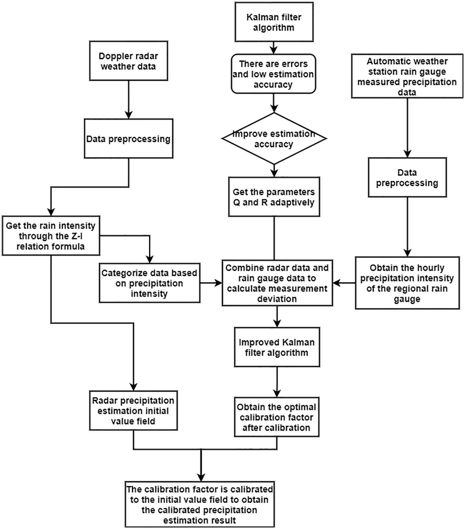
Figure 2: The overall technical route of the radar rainfall estimation model based on improved Kalman filter

3.2 Optimizing Parameter Values

When using the ordinary Kalman filter algorithm to process the rainfall estimation of Doppler radar data, we can know from the literature [19]:

Q(k)=a2(1−a12)(11)

R(k)=a3ηa4(k)(12)

In formulas (11) and (12), a1,a2,a3,a4 are the parameters of each time when participating in rainfall estimation, and η(k) represents the total number of rain gauges with precipitation measured by the automatic weather station in the k-th hour.

In general, for calculation simplicity, the state noise variance Q(k) and measurement noise variance R(k) that are substituted into the Kalman filter equation for calculation are assumed to be a priori constant values. However, different parameter values affect the accuracy of rainfall estimation to some extent [20,21].

Therefore, in order to better adapt to the more complicated rainfall estimation in the precipitation process, we decide to optimize the values of the state noise variance Q(k) and the measured noise variance R(k). We let the coefficients Q(k)andR(k) in the Kalman filter can be calculated adaptively according to the continuous observation data instead of artificially setting them as fixed constants.

It is conceivable that the value and update of the state noise variance Q(k) and the measurement noise variance R(k) are integrated into the iterative process of the Kalman filter calibration rainfall estimation model. Although the accuracy of the rainfall estimation can be improved, it is repeated Calculating the error variance, state noise variance, and measurement noise variance in the filtering process will seriously increase the amount of calculation of the Kalman filter algorithm. At the same time, the process of constantly updating numerical calculations is also extremely prone to calculation deviations, which leads to poor accuracy of the estimation results.

In view of the large amount of calculation mentioned above and the deviation of the value update process, we decide when estimating the precipitation, the data will be substituted into the improved Kalman filter calibrated rainfall estimation model batch by batch according to the result of the above classification which depends on the precipitation intensity. Take several sets of data for each type of deviation calibration factor into the improved Kalman filter that can adaptively calculate and update the state noise variance Q(k) and measurement noise variance R(k) each time. According to the type, Q  and R could be assigned optimal values when filtering the remaining data.

3.3 Kalman Filter Semi-Adaptive

The Kalman filter is adaptive, which means that the ordinary Kalman filter algorithm can automatically calculate and update the state noise variance Q(k) and measurement noise variance R(k) of each step in the system based on continuous observation data and the convergence of the Kalman filter itself.

The semi-adaptive Kalman filter is to first calculate the parameter value of each step based on the values of the previous observation data. The current calibrated optimal state noise variance Q(k) and measurement noise variance R(k) which will be substituted into the subsequent data calibration process can be obtained based on these parameters.

Define the “innovation” sequence according to the theory of Kalman filtering:

μk=Zk−X^k− =(Xk−X^k−)+vk=ek+vk(13)

X^k− represents the prior value of the bias calibration factor at time k estimated according to the bias calibration factor at time k − 1. ek represents the predicted error, that is the value of Xk minus X^k−.

According to formula (4), formula (14) can be obtained:

Zk+1−Zk=Xk+1−Xk+vk+1−vk(14)

Combine it with the state Eq. (3) to get the formula (15):

Zk+1−Zk=ωk+vk+1−vk(15)

From the basic principle of Kalman filter, we know that ωk and vk are independent of each other, random variables vk and vk+1 are independent too. So we can deduce:

D(Zk+1−Zk)=D(ωk)+D(vk+1)−D(vk)=Q+2R(16)

D represents variance. According to the deviation calibration factor at time k − 1, the deviation value of the deviation calibration factor at time k is estimated as:

X^k−=X^k−1=E[Zk−1](17)

The error variance of the forecast bias is:

Pk−=E[(Xk−X^k−)2](18)

The variance of the “innovation” sequence μk defined above [22]:

P0(K)=E{μkμk}=E{(Xk−X^k−)2}+E{vk2}=Pk−+R(19)

According to the theoretical characteristics of the Kalman filter algorithm, we can know:

limk→∞⁡Pk−=(Q+(Q2+4RQ)0.5)2(20)

Simultaneous formulas (16), (19) and (20) show that:

Q2+4RQ=(2limk→∞⁡P0(K)−D(Zk+1−Zk))2(21)

According to formulas (16) and (21), the values of Q and R can be calculated.

So far, we have basically realized the improvement of the ordinary Kalman filter algorithm. The traditional Kalman filter algorithm is adaptive and the two parameters used in the filtering process can be calculated according to the input calibration deviation to obtain the optimal parameter assignment for the subsequent filtering observation data.

4  Experiments

4.1 Datasets

First, we use the Doppler weather radar data from Nanjing, Jiangsu Province on August 16, 2021 and the data from the automatic weather station in Nanjing, Jiangsu Province at the same time period to analyze the influence of the value of the Kalman filter parameter state noise variance Q on the filtering results [23]. The test data comes from the National Meteorological Science Data Center (http://data.cma.cn/).

Subsequently, several times of the same intensity radar data obtained from the same site in Nanjing, Jiangsu Province and the data from the automatic weather station in Nanjing, Jiangsu Province during the same period were used to analyze the experimental results of the rainfall estimation based on the improved semi-automatic Kalman filter algorithm.

The maximum observation data range of Nanjing Doppler weather radar echo is 230 km, and the main data extracted is the scan data with an elevation angle of 1.5 that is completed every 6 min. The automatic weather station data mainly extracts the measured data statistics of the precipitation per hour in Nanjing.

4.2 Influence of Initial Value Parameters

In the rainfall estimation based on the improved Kalman filter, X is the one-dimensional variable precipitation, and the variances of ωk−1 and vk are Q and R respectively. In order to determine whether the values of the state noise variance Q and the measurement noise variance R have an effect on the rainfall estimation results. The experiment first adjusts the assumed values of the parameters, and compares the rainfall estimated that calibrated with different parameter values after filtering with the actual precipitation.

The observed noise variance R is also called the measurement noise variance, which is a statistical parameter. Its value is closely related to the accuracy of the data returned by the Doppler weather radar. The measurement variance can be obtained through long-term probability statistics on the data measured. In the experiment to test whether the parameter Q has an effect on the rainfall estimation result, the measurement noise variance R is set to 0.1.

It is difficult to obtain accurate data for the process noise variance Q. Therefore, in this paper, a comparative experiment is carried out on the value of the process noise parameter Q suitable for the rainfall estimation model.

Take the Doppler weather radar data on August 16, 2021 as sample data to analyze and determine the optimal value of the process noise variance Q. In this experiment, when other parameter conditions are the same, Kalman filter is performed on the parameter Q with values of 0.01, 0.1, 0.25, 0.5, and 0.75. The filtering results are shown in the following Figs. 3–7:

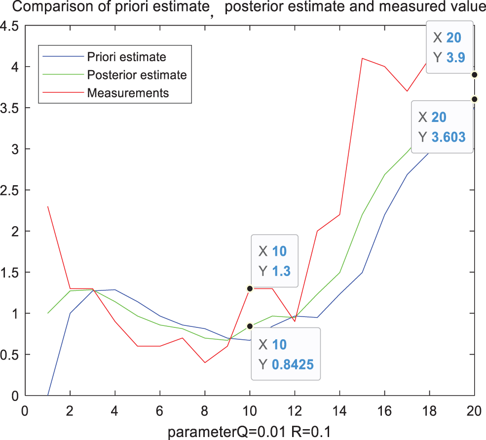
Figure 3: Filter comparison diagram when parameter Q = 0.01

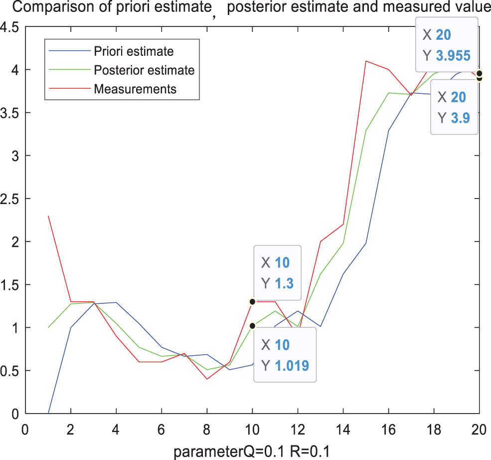
Figure 4: Filter comparison diagram when parameter Q = 0.1

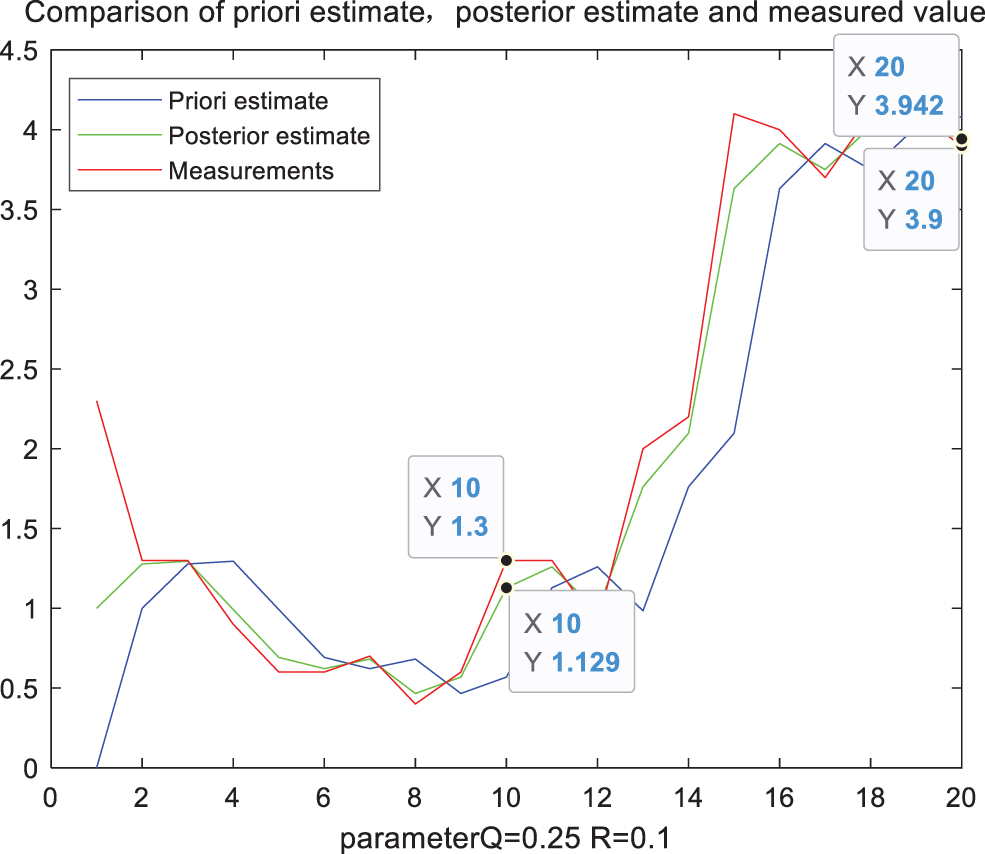
Figure 5: Filter comparison diagram when parameter Q = 0.25

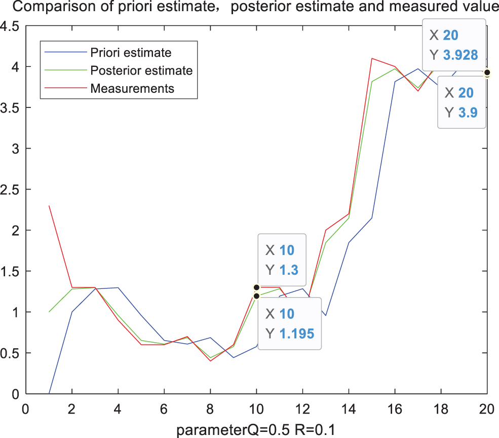
Figure 6: Filter comparison diagram when parameter Q = 0.5

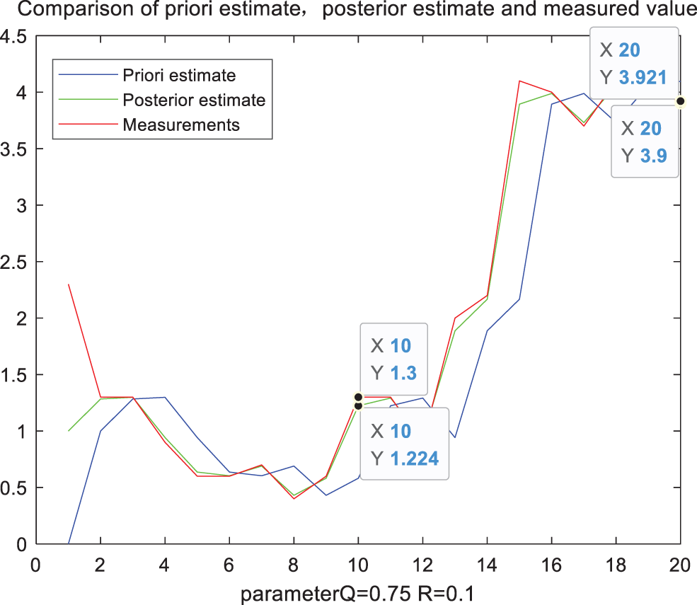
Figure 7: Filter comparison diagram when parameter Q = 0.75

Taking the measured precipitation at two points as reference in the above figure, and the specific data statistics are shown in Tab. 1. It can be seen from Tab. 1 that when Q takes different values, the filtered precipitation also has a significant impact. Gradually increase the value of Q, when the parameter Q is 0.25, the error value at the first moment is the smallest. But when it increases accordingly, the error value will increase again. However, the Q with the smallest error value at the first time corresponds to the filter calibration data error at the second time larger than the filtering result when Q is 0.1. The error at the second time is consistent with the overall trend of the error at the first time, but its best parameter Q is taken at 0.1. Therefore, we can conclude that if a fixed constant Q is always used in the entire rainfall estimation, the error effect caused by it is obvious in the different precipitation conditions at different times. It is one of the important factors leading to the lower accuracy of radar rainfall estimation.

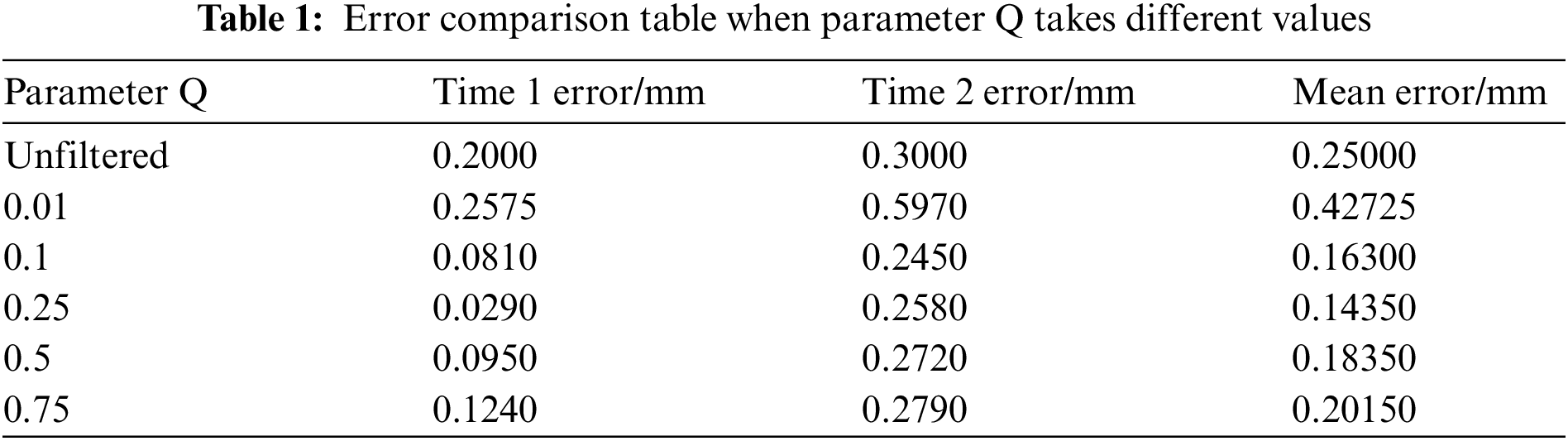
We can see that the assumed value of the parameter value Q has a significant impact on the results of the rainfall estimation. The best value of the state noise variance Q under different conditions at different times will also change to a certain extent as time changes. Therefore, we can conclude that Q(k) and R(k) which are fixed constant values affects the accuracy of precipitation estimation.

4.3 Analysis of Results

For the ever-changing and complex weather in practical applications, its parameters cannot always be consistently adapted to various environments and time periods. Therefore, the radar precipitation in the area is subjected to an improved semi-adaptive Kalman filter, and the calibrated results are compared and analyzed with the actual measurement value of the automatic weather station rain gauge in the area.

In this experiment, Several Doppler weather radar data of the same type of precipitation intensity in Nanjing City, Jiangsu Province were selected as sample data to be substituted into the rainfall estimation model for experimentation. First, the radar data obtains the rainfall estimation result according to the Z-I relationship, that is, the rainfall estimation data of the unfiltered wave. Compare the intensity of the unfiltered rainfall estimation with the actual measured value of the rain gauge in the area to obtained f which will be substituted into the rainfall estimation model based on the traditional Kalman filter and the improved Kalman filter.

In the experiment, the parameters of the rainfall estimation based on the traditional Kalman filter are set to the optimal value obtained from the above experiment. Take the data obtained from the automatic weather station rain gauge in the area as the actual precipitation. The final comparison of experimental results is shown in Tab. 2 below.

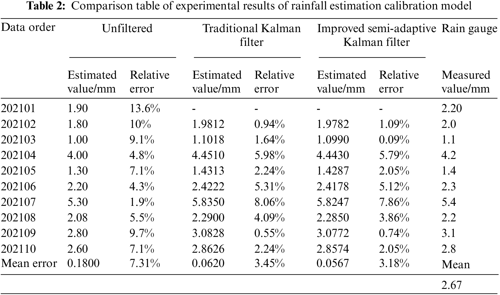
From the data in the table, we can see that the ordinary Kalman filter has significantly improved the rainfall estimation results. The average relative error of the rainfall estimation drops to 3.45%. Compared with the unfiltered rainfall estimation error, it only accounts for 47.2% of its average relative error value. The improved semi-adaptive Kalman filter's average relative error is further reduced to 3.18%, which only accounts for 43.5% of the precipitation estimate without filter wave calibration. It can be seen that the improved semi-adaptive Kalman filter algorithm has further improved the accuracy of radar rainfall estimation based on the calibration error of the ordinary Kalman filter.

5  Conclusion

In this paper, we propose a rainfall estimation model based on improved semi-adaptive Kalman filter to calibrate the rainfall estimation results, and realize the optimization of the state noise variance Q(k) and the measurement noise variance R(k) in the Kalman filter. The parameters of the model are no longer artificially set fixed values, but are calculated by the improved model based on the input observation data and updated continuously. In order to reduce the amount of calculation and improve the calibration efficiency of the rainfall estimation model, we take different types of precipitation intensities as the unit. Import data in turn and adaptively calculate the state noise variance Q(k) and measurement noise variance R(k) each time. The optimal parameter value of the current type of precipitation intensity can be obtained according to the result of the adaptive calculation, which is used as the optimal parameter of the residual deviation calibration factor. The experiments show that the state noise variance Q(k) and the measurement noise variance R(k) obtained through the improved semi-adaptive Kalman filter are more reasonable. The deviation calibration factor obtained with this method make the rainfall estimation more accurate, while avoiding tedious calculations and improving the efficiency of filter calibration.

Acknowledgement: This work was supported by the National Natural Science Foundation of China (Grant No. 42075007), the Open Grants of the State Key Laboratory of Severe Weather (No. 2021LASW-B19).

Funding Statement: The authors received no specific funding for this study.

Conflicts of Interest: The authors declare that they have no conflicts of interest to report regarding the present study.

This work is licensed under a Creative Commons Attribution 4.0 International License, which permits unrestricted use, distribution, and reproduction in any medium, provided the original work is properly cited.