| Journal of Renewable Materials |
DOI: 10.32604/jrm.2022.017506
ARTICLE
Understanding the Impacts of Plant Capacities and Uncertainties on the Techno-Economic Analysis of Cross-Laminated Timber Production in the Southern U.S.
1Department of Forestry and Environmental Resources, North Carolina State University, Raleigh, 27606, USA
2Department of Forest Biomaterials, North Carolina State University, Raleigh, 27606, USA
*Corresponding Author: Kai Lan. Email: klan2@ncsu.edu
Received: 15 May 2021; Accepted: 04 June 2021
Abstract: Understanding the economic feasibility of cross-laminated timber (CLT), an emerging and sustainable alternative to concrete and steel, is critical for the rapid expansion of the mass timber industry. However, previous studies on economic performance of CLT have not fully considered the variations in the feedstock, plant capacities, manufacturing parameters, and capital and operating costs. This study fills this gap by developing a techno-economic analysis of producing CLT panels in the Southern United States. The effects of those variations on minimum selling price (MSP) of CLT panels are explored by Monte Carlo simulation. The results show that, across all the plant capacities from 30,000 to 150,000 m3/year, the MSP ranges from $345 to $609/m3 with a ±6%–9% range caused by the variations in feedstocks, key manufacturing parameters, capital and operating cost. The MSP decreases significantly along the increasing capacities. A sensitivity analysis exhibits that the lumber price, lumber preparing loss, plant capacity, and the installed costs of layering and gluing, finishing, and miscellaneous, are the top driving factors to CLT MSP. Supported by Geographic Information System, this study also studies the transportation cost of delivering CLT to customers under three CLT demanding levels (1%, 5%, 15%). The results show that the transportation cost is 1%–8% of the MSP. Lower demanding level or higher plant capacity can increase the transportation cost due to average longer delivering distance. When considering the delivered cost that sums MSP and transportation cost, larger plant capacity does not necessarily generate lower delivered cost.
Keywords: Cross-laminated timber; techno-economic analysis; plant capacity; uncertainty; minimum selling price
Currently, the reinforced concrete and steel dominate the structural systems of mid-rise buildings (e.g., commercial buildings) in North America [1,2]. Recently, cross-laminated timber (CLT) has attracted increasing attention for mid-rise buildings as an environmentally sustainable alternative to reinforced concrete and steel [3–6]. CLT is a prefabricated mass timber product with odd lumber (sawn lumber or structural composite lumber) layers (typically 3, 5, or 7) stacked crosswise (typically 90°) to form a solid panel [1,7–10]. The typical dimension of CLT panels can reach 0.30–3.05 meters in width, 0.10–0.25 meters in thickness, and up to 18 meters [11,12]. Over traditional reinforced concrete and steel, CLT has shown advantages in fire resistance and thermal performance [13–17], acoustic performance [12,18–21], mechanical properties (e.g., bending stiffness and strength) [22–26], lower density [20,21,27], faster installation process [12,23,28], recyclability [3,29], and potential carbon storage [30,31]. Driven by these advantages, in the recent decade, the CLT market has been growing [11,32]. Energias reported that the global CLT market size was $641 million in 2017 and forecasted to be $1,833 million by 2024 with a compounded annual growth rate (CAGR) of 16.2% [33]. In North America, Ganguly et al. evaluated the demand for CLT panels in the Pacific Northwest (PNW) region to be 0.19 million m3/year by 2035 compared to around 0.008 million m3/year in 2016–2018 (less than 1% of annual PNW timber harvest) [32]. In the study by the Council of Western State Foresters (CWSF), the CLT demand in the CWSF region (17 Western US states and 6 US affiliated Pacific Islands) was estimated to be 0.26 million m3/year by 2020 and 0.52 million m3/year by 2025 [34]. In North America, by 2016, there were five CLT manufacturers in operation (three in the U.S. and two in Canada). The CLT manufacturer number in North America now increases to eleven among which five are in Canada (Structurlam Mass Timber Corporation, Nordic Structures, Kalesnikoff Mass Timber, Leaf Engineered Wood Products, and Element5 Co.,) and six are in the U.S. (IB X-Lam USA, Johnson Wood Innovations, SmartLam, Freres Lumber Co., Vaagen Timbers, and Sterling Lumber) [35–37]. Under this situation, understanding the economic viability of the CLT panels is important for the expansion of the CLT industry.
To evaluate the economic feasibility of CLT panels, techno-economic analysis (TEA) can be used as a widely adopted tool [38–40]. Two previous TEA studies explored the economic performance of CLT panels. Brandt et al. explored the minimum selling price (MSP) of 1 m3 CLT panels from softwood lumber and showed that the MSP was $652/m3 and $536/m3 for 52,000 and 87,000 m3/year plant, respectively [4]. In 2010, Bédard et al. evaluated the production cost of CLT from spruce lumber at a 30,000 m3 CLT/year plant and concluded the cost was $679/m3 [41]. Another study by FPInnovations in 2013 briefly estimated the average CLT production cost to be $678/m3 [11]. However, previous TEA studies on CLT have not considered the variations in lumber feedstock (e.g., moisture content, lumber price), manufacturing parameters (e.g., material loss, resin usage), and transportation cost of delivering CLT panels which is dependent on varied market demanding levels and plant capacities. These variations may have large impacts on the economic viability of CLT. Strengthening the understanding of the impacts of those variations can help the future designing and planning of the CLT plant and identify the key drivers of the cost, especially under varied future market conditions.
This study addressed the challenge by conducting a TEA for producing CLT from softwood lumber in the Southern U.S. MSP of CLT panels was selected as the economic indicator. This study also investigated the transportation cost of delivering CLT from the plant to consumers. The transportation route was optimized by a linear programming model where the road network information was provided by Geographic Information System (GIS). The mass and energy data of the CLT plant were generated from a process-based simulation model. The data ranges of key parameters were collected from the literature to analyze their impacts on the economic performance. To model these variations, Monte Carlo simulation (MCS) was used [38,42]. Scenario analysis was conducted to evaluate the effects on MSP and delivered cost (MSP plus transportation cost of delivering CLT) under different plant capacities and market demanding levels.
In this study, a TEA was performed to evaluate the minimum delivered cost of 1 m3 CLT panel which consists of two components, MSP out of the CLT plant gate and delivering transportation cost to the construction site. The MSP was calculated in a discounted cash flow rate of return (DCFROR) analysis, a widely adopted economic analysis tool in varied industries (see Section 2.2) [43–45]. The MSP is a critical indicator in evaluating the economic feasibility of a product by representing the minimum product selling price to reach the breakeven point in the cash flow [45]. In other words, the MSP indicates the lowest selling price to cover all the production costs. In the DCFROR analysis, the capital costs and operating costs of the CLT plant were calculated based on the mass and energy balance generated by the process simulation model. The transportation cost was estimated by a mathematical programming model where the transportation distance was provided by the GIS model (see Section 2.3).
Fig. 1 shows the system diagram of the CLT plant. After softwood lumber arrives at the plant, lumber is unloaded by the forklift and stored in the warehouse. The forklift transfers lumber from the storage site to the lumber feeding system. In lumber preparation, lumber undergoes the visual grading and grouping process to ensure that the lumber in longitudinal layers reach visual grade No. 2 and the lumber in transverse layers reach visual grade No. 3 [46]. Then the lumber moisture content is measured. As required by the ANSI/APA PRG 320-2019 standard, the moisture content of lumber need to be 12 ± 3%, which is assumed to be the uncertainty range of lumber moisture content in this study (see Tab. 1) [46]. Following the grading and moisture detecting, lumber is trimmed or re-cut to remove defects [47,48]. The waste from lumber preparation can vary significantly based on previous studies and highly depend on the feedstock suppliers, but is controllable by selecting qualified suppliers [12,41,48]. The range of material loss in lumber preparation is documented in Tab. 1. The selected and grouped lumber is temporally stored for the next step, end-jointing. In the end-jointing, lumber is longitudinally end-jointed to make long continuous lumber [24]. In this study, finger-jointing was assumed to be the end-jointing type. Four-side planing is needed to meet the requirement of thickness tolerance for better bonding results [7,24]. The longitudinally assembled lumber is layered and glued for face bonding [28]. The resin was selected to be melamine formaldehyde (MF), as a commonly used resin in finger-jointing and face-bonding. The MF usage in this study was collected from the literature (see Tab. 1) [12,24,48,49]. After pressing, the finishing step includes planing and end cutting. Planing is needed to remove any excess resin and final uneven surfaces. Since CLT panels are highly prefabricated and customized for fast erection and minimal onsite cutting, Computerized Numerical Control (CNC) is commonly used [50]. CLT is then packaged and ready for transport to the construction site.
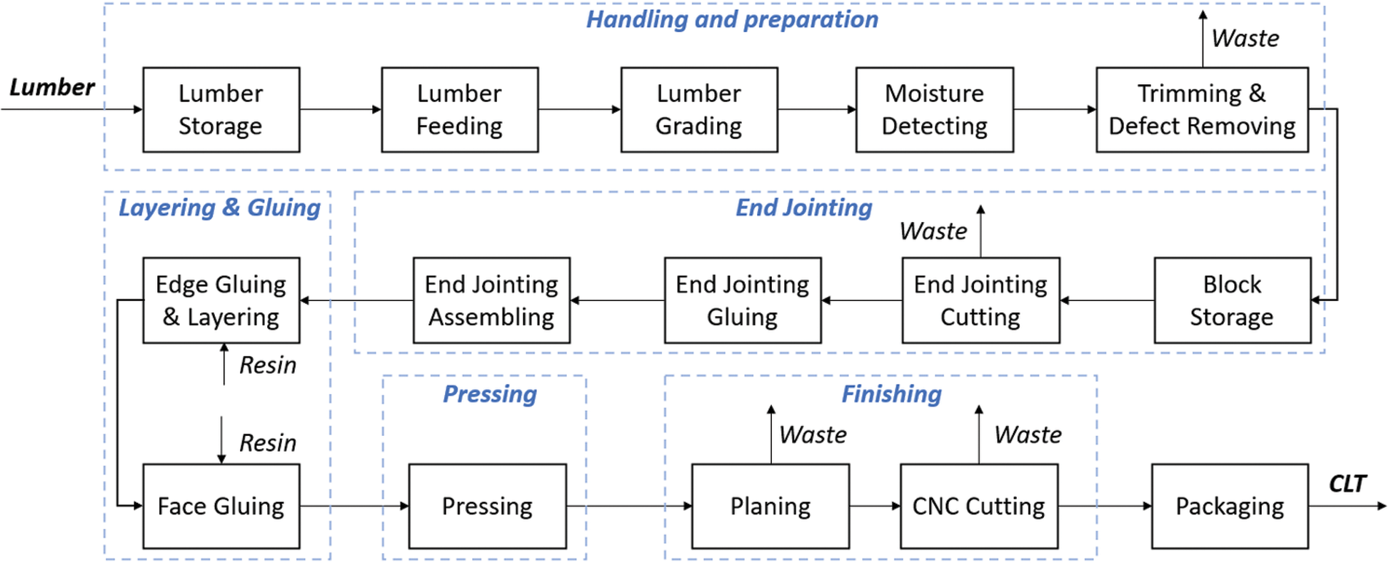
Figure 1: Flow diagram of the CLT plant
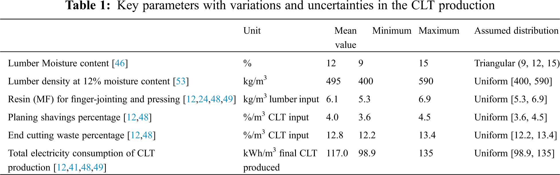
The variations and uncertainties of the key parameters for the CLT production were collected from the literature and documented in Tab. 1. The diesel consumption of hauling and conveying materials between unit operations was assumed 1.3 L/m3 final CLT produced [51–53].
2.2 Economic Analysis of CLT Plant
This economic analysis focuses on the CLT plant with capacities ranging from 30,000–150,000 m3 per year [4,41]. The mass balance data were fed into the economic analysis to determine the variable operating costs and equipment sizes that were used to scale the original purchased costs. The original purchased costs along with installing factors and scaling factors of each equipment were collected from the literature and manufacturer data. This study follows the nth plant assumption which means a similar plant has been previously operated without unexpected startup delays and capacity loss [54,55]. Following Sections 2.2.1 and 2.2.2 will describe capital expenditures (CAPEX) and operating expenditures (OPEX).
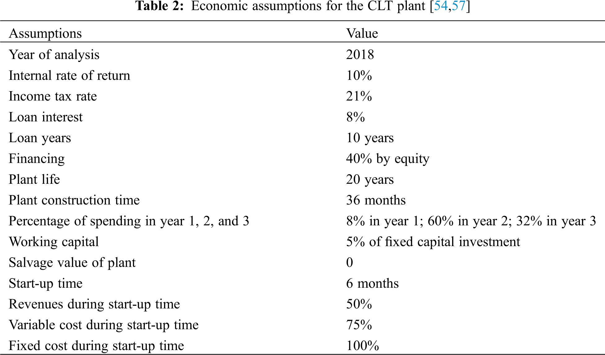
A DCFROR analysis was established in EXCEL to calculate the MSP under varied scenarios [39,43–45,56]. Tab. 2 lists the assumptions and parameters used in the DCFROR analysis [54,57]. In the DCFROR spreadsheet, MSP is derived by setting IRR to be 10% and the Net Present Value (NPV) to be zero [45]. NPV was calculated by Eq. (1) [58,59], where atis the cash flow at time t with IRR r.
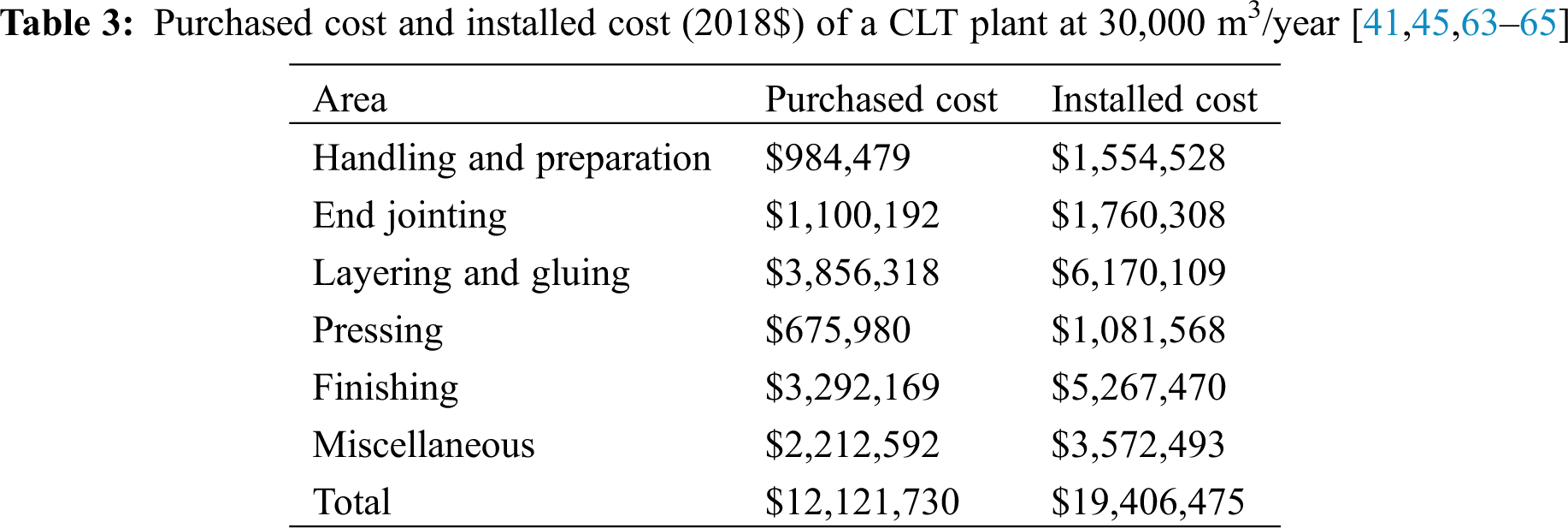
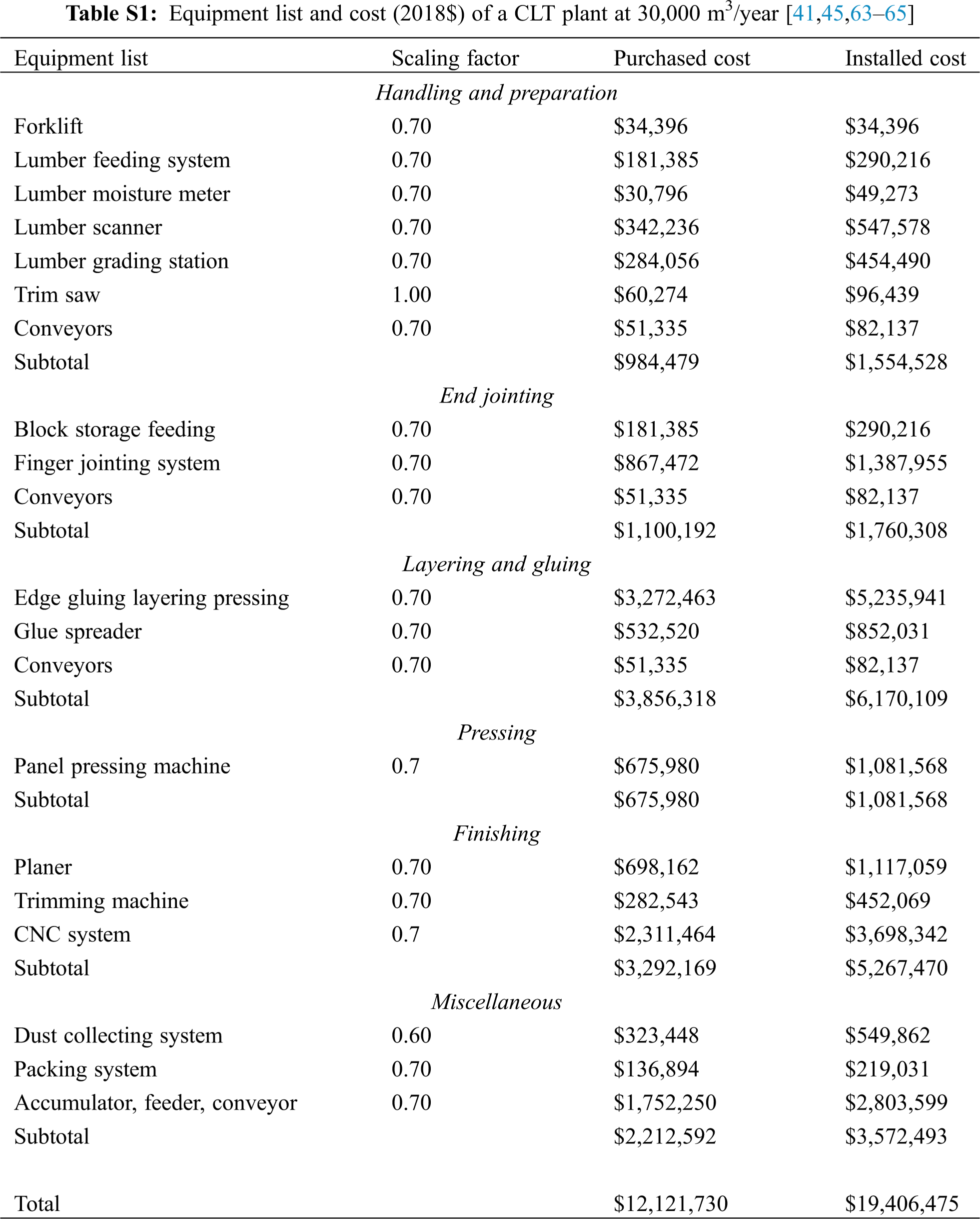
The original purchased costs along with installing factors and scaling factors of each equipment were based on the literature and manufacturer information and then were scaled to the capacities by using scaling factors in this study. Tab. 3 shows the purchased costs and installed costs of the major areas at 30,000 m3 CLT/year as an example. The detailed equipment list with scaling factors, purchased costs, and installed cost is available in Appendix A. Tab. S1. To adjust equipment purchase costs to the year of analysis 2018, plant cost indices by Chemical Engineering Magazine are used [60]. To account for the uncertainties of the equipment costs, this study adopts the data range to be ±30% which is commonly estimated as the accuracy of this scaling method in TEA [4,61].
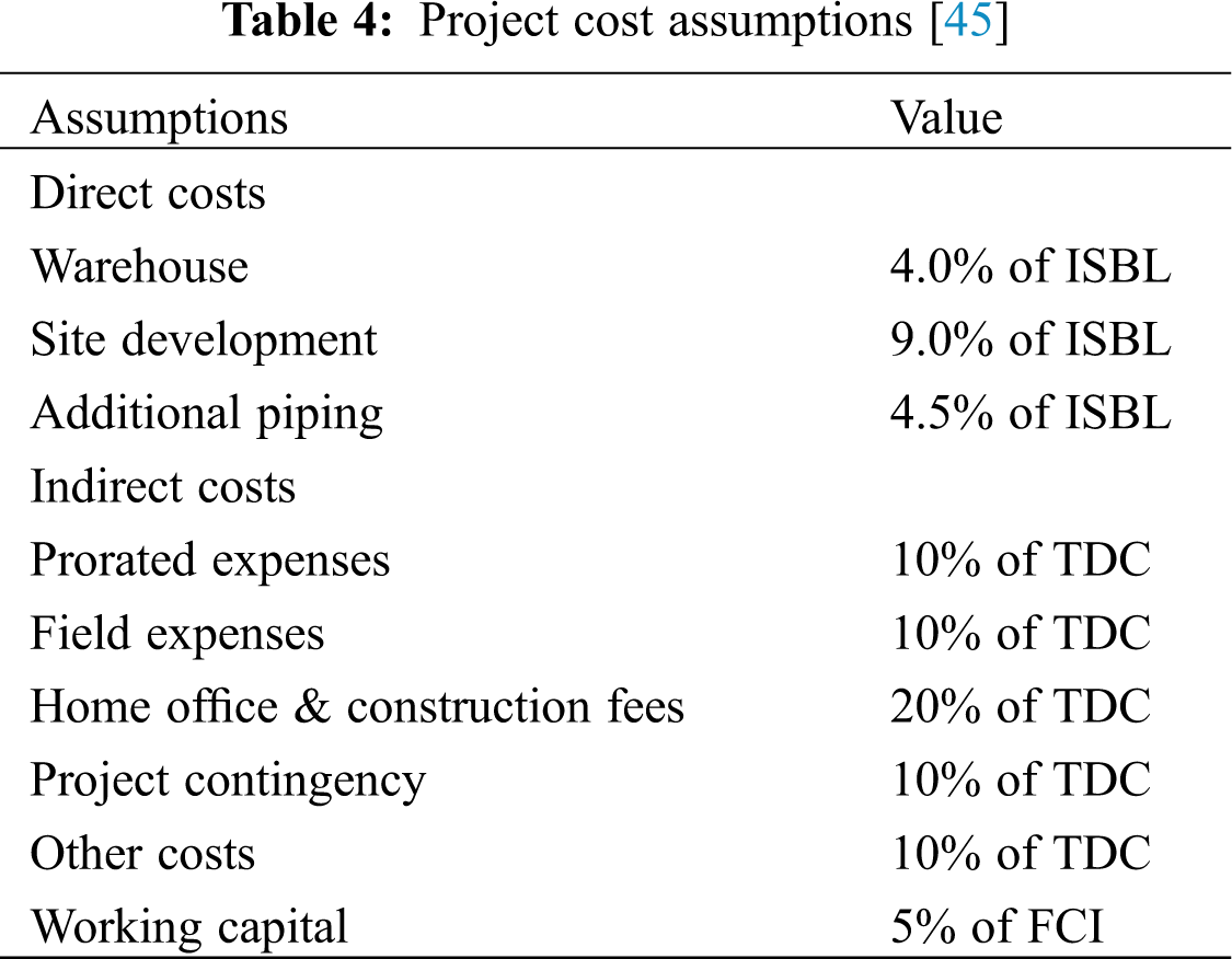
After the total installed cost (TIC) has been decided, there are several direct costs and indirect costs. These direct costs include warehouse, site development, and additional piping. Then the total direct costs (TDC) are the sum of TIC and these direct costs. The indirect costs contain prorated expenses, home office and construction fees, field expenses, project contingency, and other costs, which are calculated based on TDC [45]. Fixed capital investment (FCI) sums TDC and indirect costs. The land cost is assumed to be 60 acres at $14,000 per acre [62]. Tab. 3 summarizes the assumptions in baseline costs related to direct and indirect costs. Tab. 4 lists the project cost assumptions.
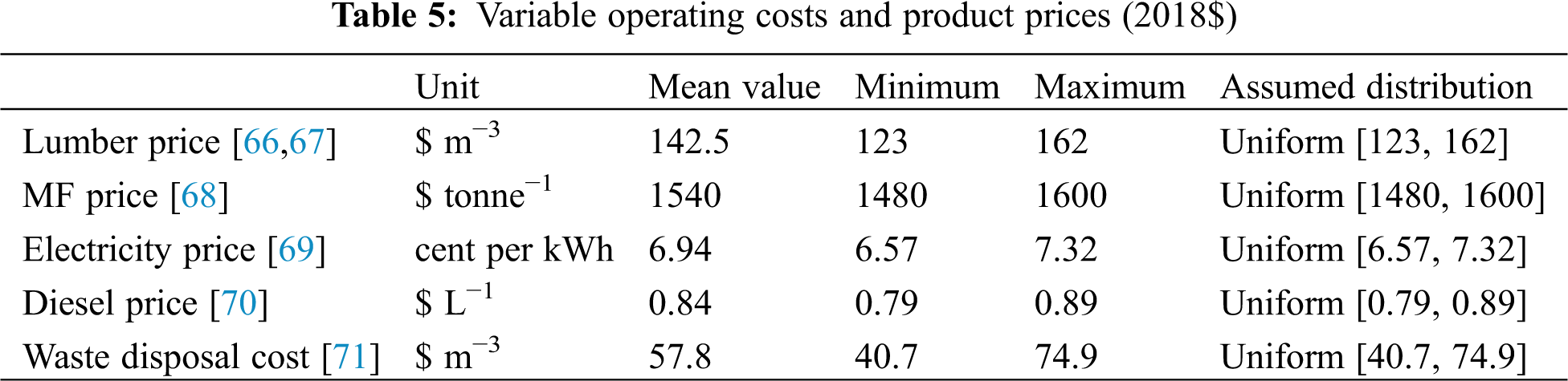
The operating costs of the CLT plant contain two components. One is variable operating costs, including raw materials, waste stream charges, and fuel consumption. The other one is fixed operating costs, including labor cost and other overhead costs (i.e., maintenance and property insurance). For variable operating costs, the quantities of raw materials, waste streams, and energy consumption were decided by the process simulation. The variations and uncertainties in the prices of raw materials, waste stream charges, and fuels were collected from the literature and documented in Tab. 5 [66–71]. If the price is not in the year of analysis, then the Producer Price Index for chemical manufacturing is used to adjust the original prices [72]. The lumber price data were determined by the price range of 2018 in the U.S. [66,67]. It is noticeable that the lumber price could have much higher fluctuations. For example, the highest lumber price in 2020 under the COVID-19 pandemic situation recorded over $400/m3 [66,67].
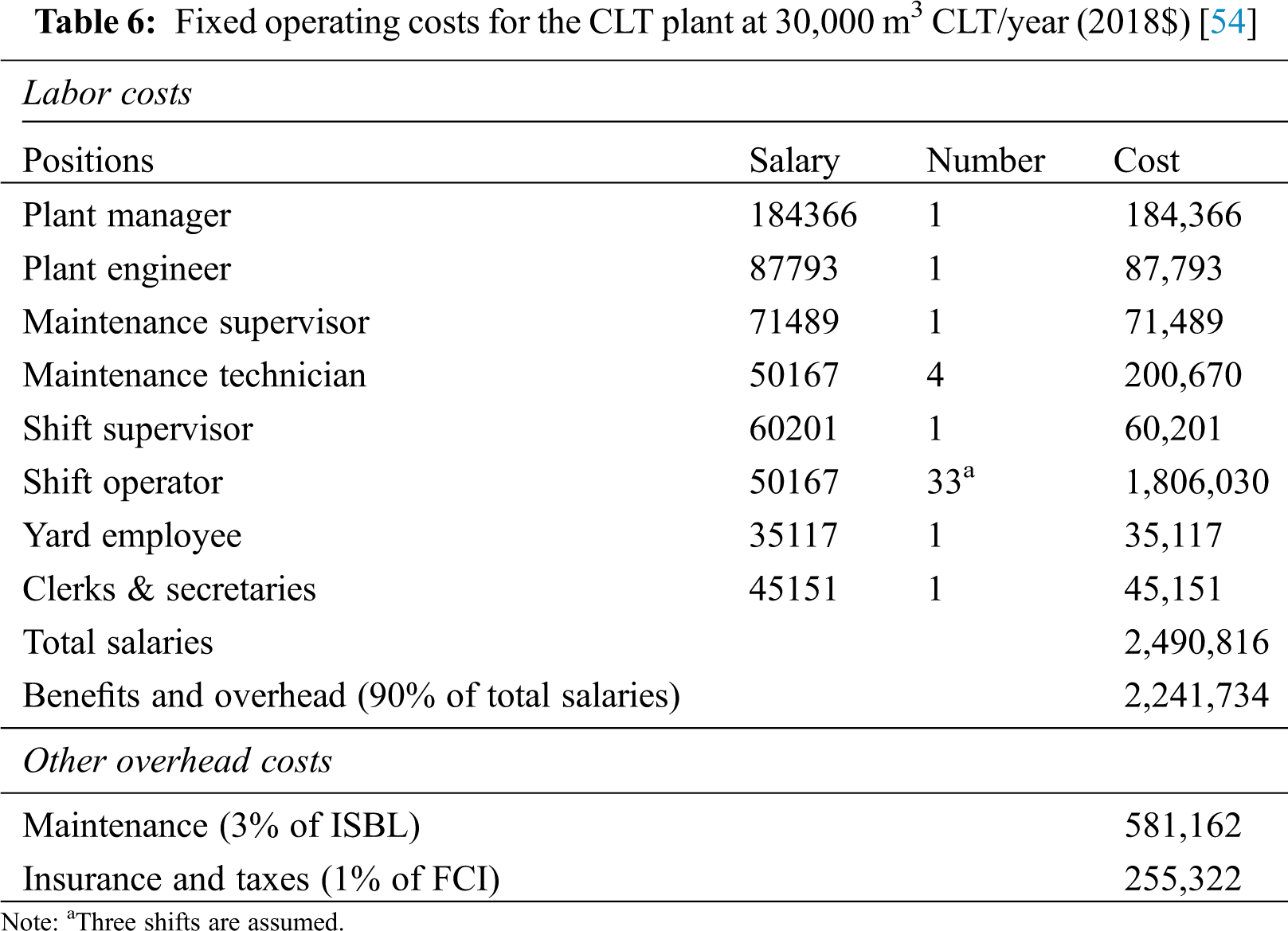
For fixed operating costs, Tab. 6 exhibits the labor costs and other overhead costs at 30,000 m3 CLT/year. The positions and salaries are based on the reports by the National Renewable Energy Laboratory (NREL) [54]. To adjust the salaries to the year of analysis, the labor index from the Bureau of Labor Statistics was used [73]. In this study, three shifts are assumed for the CLT plant. To account for the variations in operators needed, it is assumed 10–13 operators per shift for the plant at 30,000 m3/year.
2.3 Transportation Cost of Delivering CLT
The market demanding of CLT panels in the southern U.S. is estimated by assuming the market share of commercial buildings at a county level based on the literature data [11,34,41,74,75]. Three different market demanding levels are modeled in this study: 1%, 5%, and 15%, representing low, medium, and high demanding level, respectively [11,34,41]. The annual CLT demanding at the county level in the southern U.S., is estimated by Eq. (2).
Di is the CLT demanding in county i; Acommercial,i is the annual newly constructed floor area (m2) of commercial building in county i; DL is the market demanding level of CLT (1%, 5%, or 15%); F is the CLT usage factor (0.167 m3 CLT per m2 floor area) that is evaluated based on the average value of the literature data [1,27,76,77]. Acommercial,iis estimated by using the average U.S. new commercial building area per capita based on the Commercial Buildings Energy Consumption Survey (CBECS) data by U.S. Energy Information Agency (US EIA) [75]. In this study, the commercial buildings include traditional commercial buildings (e.g., stores, restaurants, warehouses, and office buildings) and hospitals, institutions, and buildings for religious worship, following the same definition given by US EIA [75]. An example of the county-level demanding results (1,339 counties) at 1% demanding level is presented in Fig. 2 (the results of 5% and 15% demanding levels are available in Appendix B. Figs. S1 and S2).
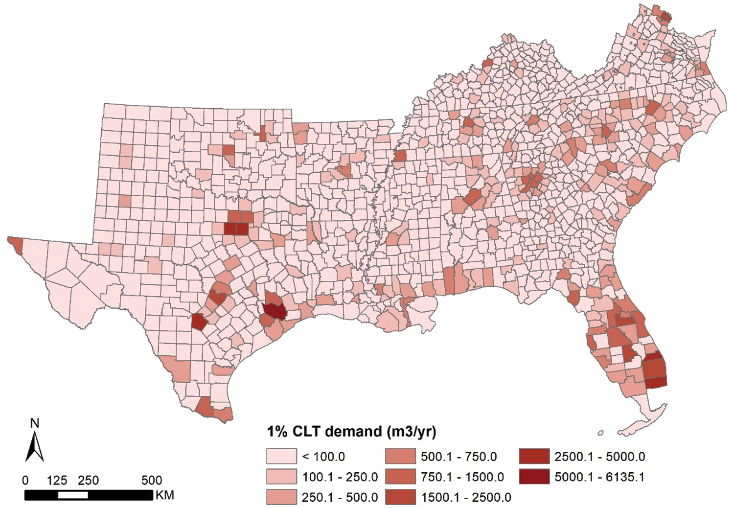
Figure 2: County-level CLT demanding results at 1% demanding level in the Southern U.S.
To estimate the travel cost at the county level, road distances between the CLT plant and geometric centers of counties within the whole south region were derived through Network Analysis in ArcGIS 10.6 [78]. In the road network analysis, the primary and secondary road system were considered and downloaded from the 2018 TIGER/Line shapefiles by US Census Bureau [79] (see Appendix B. Fig. S3). The primary roads were the limited-access highways within the interstate highway system or under State management, and the secondary roads were main arteries within the U.S. Highway, State Highway, and County Highway systems [80]. For the average truck speed on two types of roads, it was assumed to be 113 km/h (70 mile/h) for all roads that contained “Hwy” (i.e., highway) in their full name and 89 km/hr (55 mile/h) for other non-highway roads, based on the report of U.S. Department of Transportation [81].
2.3.3 Transportation Cost Rate
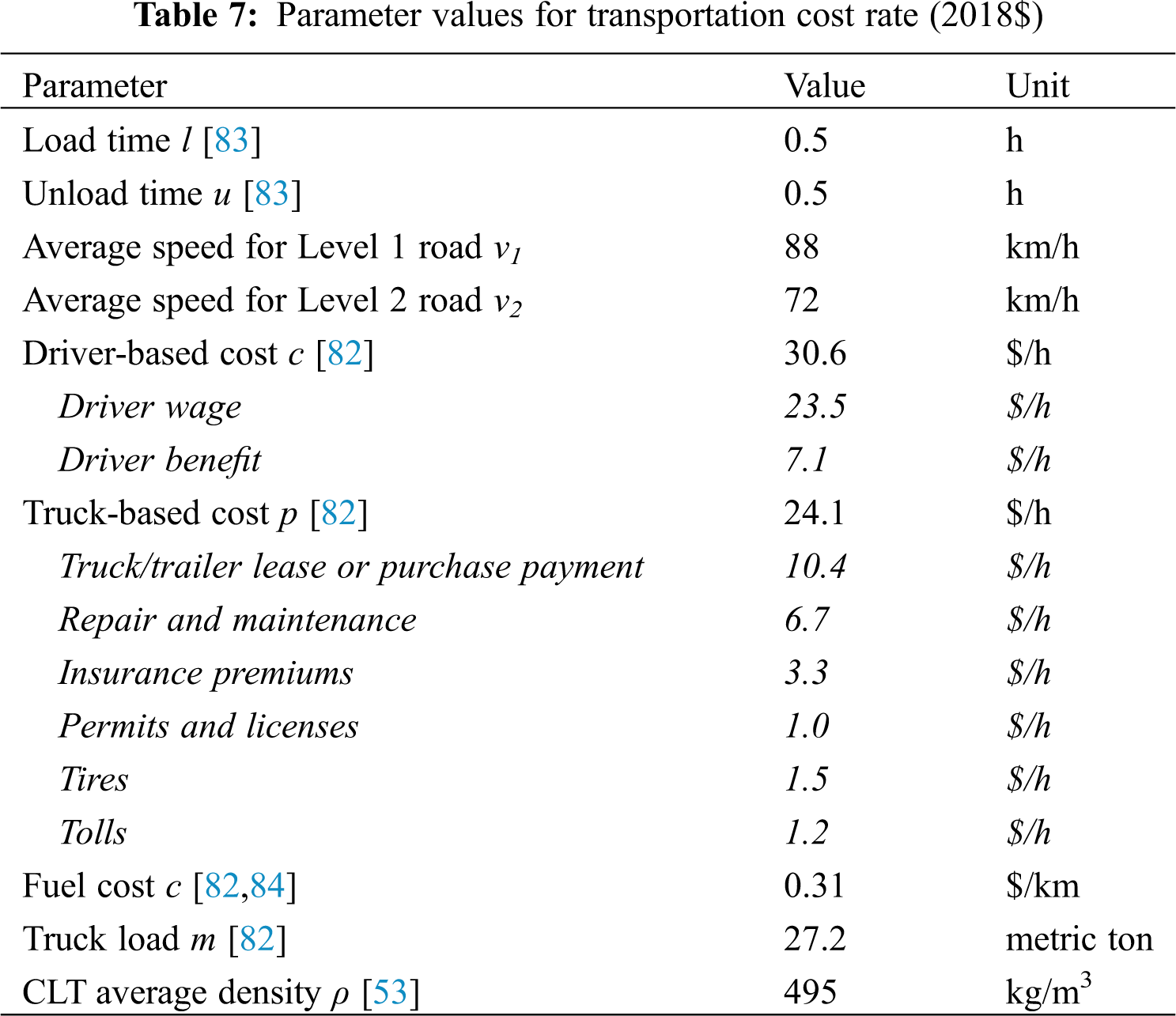
The transportation cost Ti ($/m3) for delivering 1 m3 CLT panels from the plant to county i (round trip) is estimated based on Eq. (3) [82,83]. The assumed values for the parameters in Eq. (3) are documented in Tab. 7. l and u is load time and unload time, respectively [83]. L1 and L2 the transportation distance of primary (i.e., Level 1) and secondary (i.e., Level 2) road, which is determined by the GIS model as shown in Section 2.3.2 v1 and v2 depict the average speed for Level 1 and Level 2 road. c describes the driver-based cost, including driver wages and benefits [82]; p is truck-based cost, including truck/trailer lease or purchase payment, repair and maintenance, insurance premiums, permits and licenses, tires, and tolls [82]; f is fuel cost based on the American Transportation Research Institute data (6.3 miles per gallon (2.7 L/km) for 60,00 lb operating weight) [82] and diesel price ($3.18/gallon) by US EIA [84]. m is the weight load of CLT panels with an assumption of for 60,000 lb (27.2 metric ton) [82,83]; ρ is the average density of CLT panels.
2.3.4 Least-Cost Route Determined by LP Model
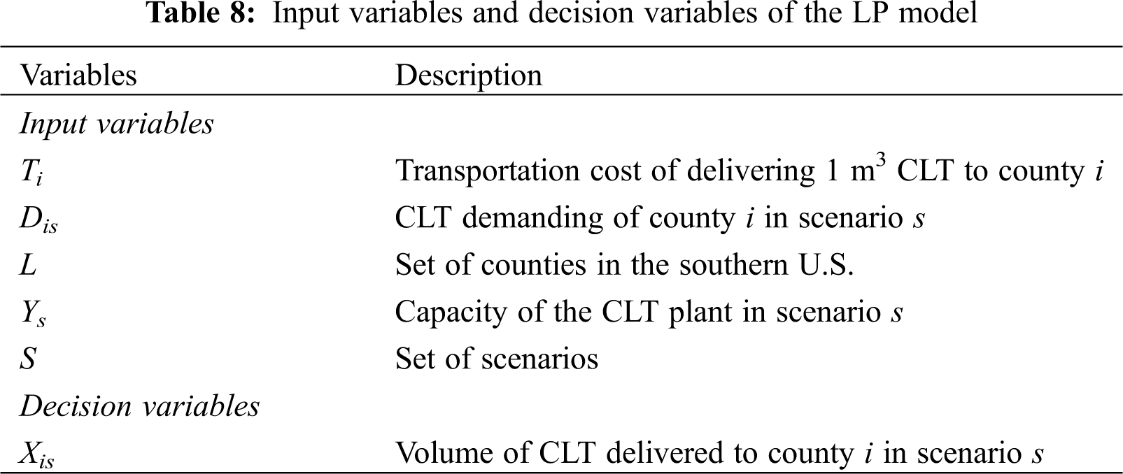
An LP mathematical model was adopted to minimize the transportation cost of delivering the CLT panels. The input variables and decision variables are listed in Tab. 8. CLT demanding of county i in each scenario, Dis, is derived based on the results of Section 2.3.1; the transportation cost Ti is derived from the results of Section 2.3.3. This study includes total 1,339 counties in L, 7 capacities of the CLT plant, and 21 scenarios in S (see Section 2.3.1). In this study, the LP problem is solved in MATLAB 2018 for each scenario.
There are two constraints involved in this problem. In constraint 1, the volume of delivered CLT panels to county i is no larger than the CLT demanding of county i in each scenario.
The scenario analysis, as shown in Tab. 9, was designed to explore the impacts of variations in plant capacity and CLT market demanding levels on the economic performance of producing CLT. The impacts of variations in other process parameters were explored by Monte Carlo simulation [48]. In this study, Monte Carlo simulation was performed for 1,000 iterations in each scenario using the probability density functions of parameters as shown in Tabs. 1, 3, and 6.
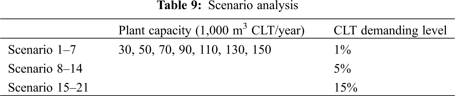
Fig. 3 exhibits the installed costs in each area, other direct cost, and indirect cost at varied plant capacities (30,000–150,000 m3/year). The error bars represent the 5th–95th percentile value range (P5–P95) of total capital investment from the Monte Carlo simulation. For varied plant capacities, increasing the capacity from 30,000 to 150,000 m3/year only raises the capital cost by 203%. Thus, increasing the plant capacity can lead to lower capital cost on a per cubic meter CLT basis. This further leads to the main driver of the decreasing MSP of CLT when increasing plant capacities (see Fig. 4). Among the installed costs of the equipment, layering and gluing (17% of the total capital investment), finishing (15% of the total capital investment), miscellaneous (9%–10% of the total capital investment) are the major components. The other three areas account for less than 5% of the total capital investment. Besides the installed costs of equipment, the other direct cost (9% of the total capital investment) and indirect cost (38% of the total capital investment) contribute significantly to the capital investment. In this study, the variations in the equipment costs lead the total capital investment to vary 10% by P5–P95. Though the result range is smaller than the uncertainty range of equipment cost (±30%), the uncertainty in capital investment needs to be considered in implementing the CLT plant.
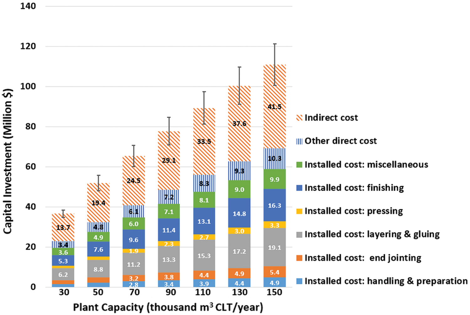
Figure 3: Capital investment of the CLT plant under varied capacities
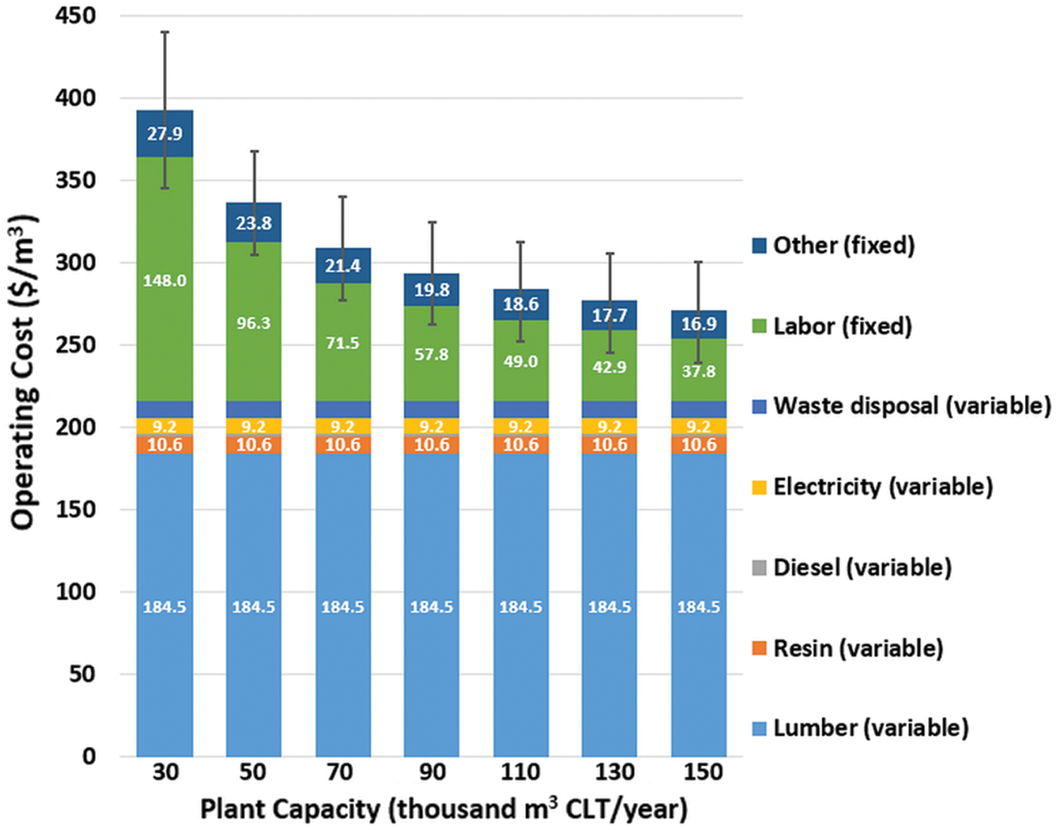
Figure 4: Operating cost of the CLT plant under varied capacities
Fig. 4 shows the operating cost of producing 1 m3 CLT under varied capacities which consists of variable and fixed operating cost. The error bars represent the P5–P95 value range. Since the variable operating cost depends on 1 m3 product basis, the variable operating cost does not change with varied plant capacities. Among the variable operating costs, the lumber cost is the dominant part accounting for 85% of the total variable operating cost and 47%–68% of the total operating cost. The other material costs and energy costs are minor (less than 8% of the total operating cost). Hence, the lumber price can be a key factor that determines the total operating cost. On the other hand, the fixed operating cost, including labor cost and other fixed cost (maintenance, insurance and taxes), decreases along with the increased plant capacity. From 30,000 to 150,000 m3/year, the labor cost reduces from $148.0 to $37.8 per m3 CLT produced, and accounts for over 69% of the fixed operating cost. Hence, increasing the plant capacity can lead to the reduction of operating cost, which is a similar trend with the capital cost.
Fig. 5 shows the MSP of CLT at varied plant capacities. The box stands for the P5–P95 value range of the Monte Carlo simulation results with tails representing the minimum and maximum results. The overall MSP of CLT panels ranges from $345 to $609/m3 across all the capacity cases. Expanding the CLT plant capacity can significantly reduce the MSP of the CLT panels. For example, the median value of MSP at 30,000 m3/year is $571/m3 ($534–$609/m3 P5–P95), compared to the median value $376/m3 ($345–$410/m3 P5–P95) at 150,000 m3/year. This phenomenon is mainly driven by the reduction of capital cost and labor cost when the capacity is increased as mentioned above (see Figs. 3 and 4). The results presented in this study stay aligned with the literature data, approximately $536–$900/m3 [4,11,41]. The difference can be caused by varied wood type, lumber cost, labor employment, and plant location and capacity [4,11,41]. The uncertainties and variabilities from the manufacturing parameters, equipment cost, and operating cost, lead to the results varying by 6%–9% (based on P5 and P95).
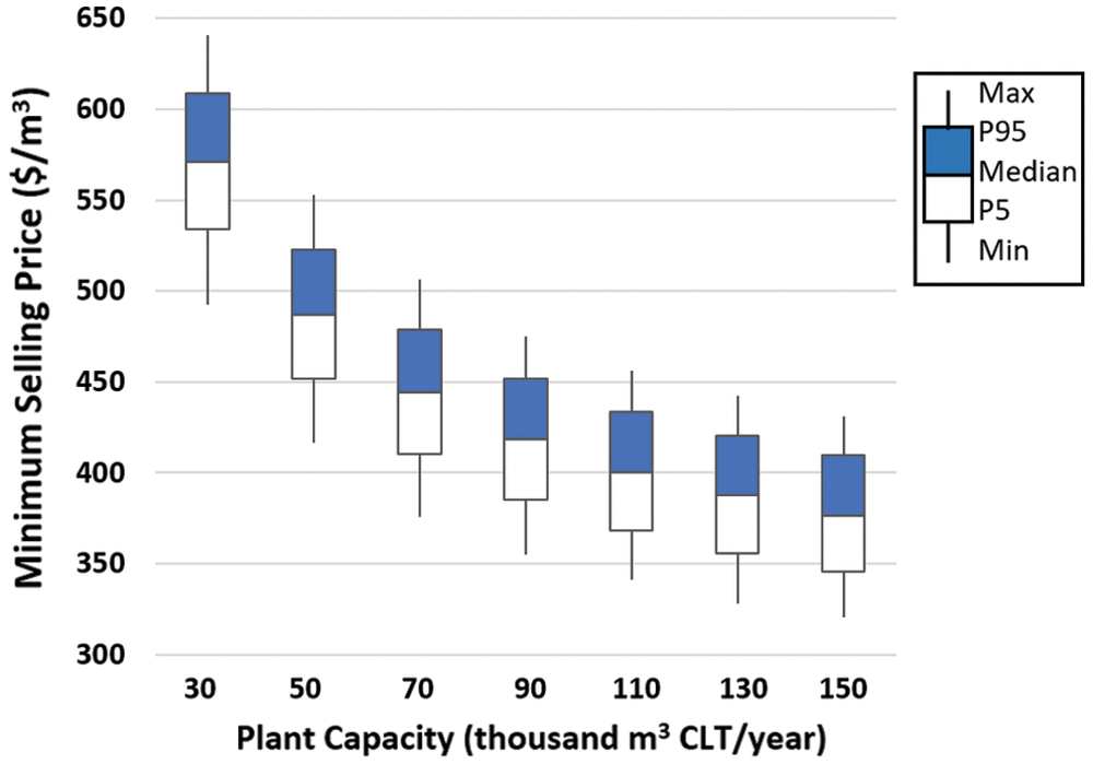
Figure 5: The minimum selling price of CLT at varied plant capacities
Fig. 6 shows the delivered cost of CLT panels at varied plant capacities and demanding levels, with error bars showing the range of P5–P95. In Fig. 6, the delivered cost consists of MSP (solid bars) and transportation cost (pattern filled bars) at three demanding levels, namely 1% (orange bars), 5% (blue bars), and 15% (grey bars). First, compared to the MSP, the transportation cost of delivering the CLT panels is much smaller, accounting for 1%–8% of the delivered cost across all the cases. Second, the transportation cost increases as the demanding level decreases or the plant capacity increases. This is due to the decreased demanding level or increased plant capacity leads to longer transportation distances to deliver the CLT panels. For example, for a 150,000 m3/year plant, the transportation cost is $33/m3 for 1%, $15/m3 for 5%, and $10/m3 for 15% demanding level. For 1% demanding level, increasing the capacity from 30,000 to 150,000 m3/year raises the transportation cost from $15 to $33/m3. Third, when considering varied demanding levels, larger plant capacity does not necessarily generate lower delivered cost. For example, the delivered cost at 150,000 m3/year with 1% demanding level ($410/m3 mean value) is $23 higher than 130,000 m3/year with 15% demanding level. Hence, the results show the necessity of considering the potential demanding conditions in implanting CLT plants.
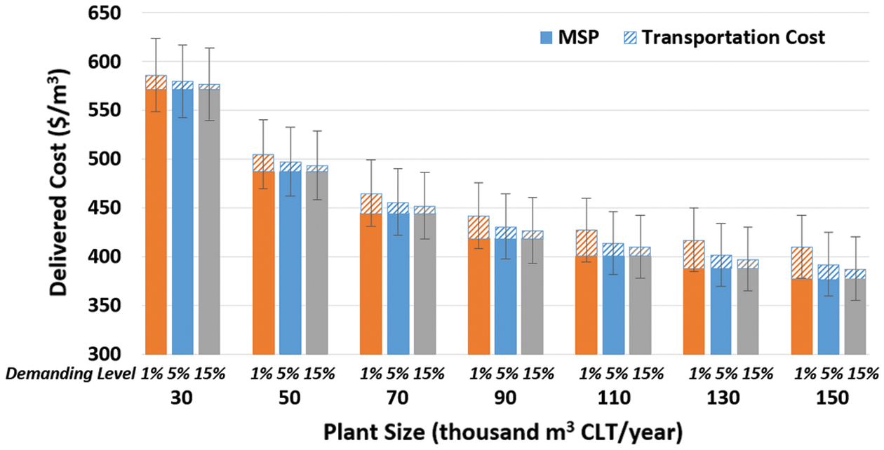
Figure 6: The delivered cost of CLT at varied plant capacities and demanding levels
To further identify the key drivers of the economic feasibility for CLT panels, this study conducted a sensitivity analysis. The baseline was chosen as the 110,000 m3/year plant as shown in Fig. 7. In the sensitivity analysis, the parameters can be categorized into three groups, manufacturing parameters, operating cost parameters, and capital cost parameters. Among manufacturing parameters, the plant capacity and the lumber preparing loss are the key driving factors that affect the MSP. A potential increase in the preparing loss (due to trimmed defects or lumber below the quality requirement) from 7% to 14% can lead to a $19/m3 increase in MSP. Lumber price, the largest portion of operating costs (see Fig. 4), is another key driver for the MSP. Hence, lowering the feedstock cost, choosing qualified feedstock, and reducing the loss in lumber preparation can be potentially effective strategies to reach lower MSP. For the capital costs, the installed costs of layering and gluing, finishing, miscellaneous are among the top ones that affect the MSP, which stays aligned with the results shown in Fig. 3.
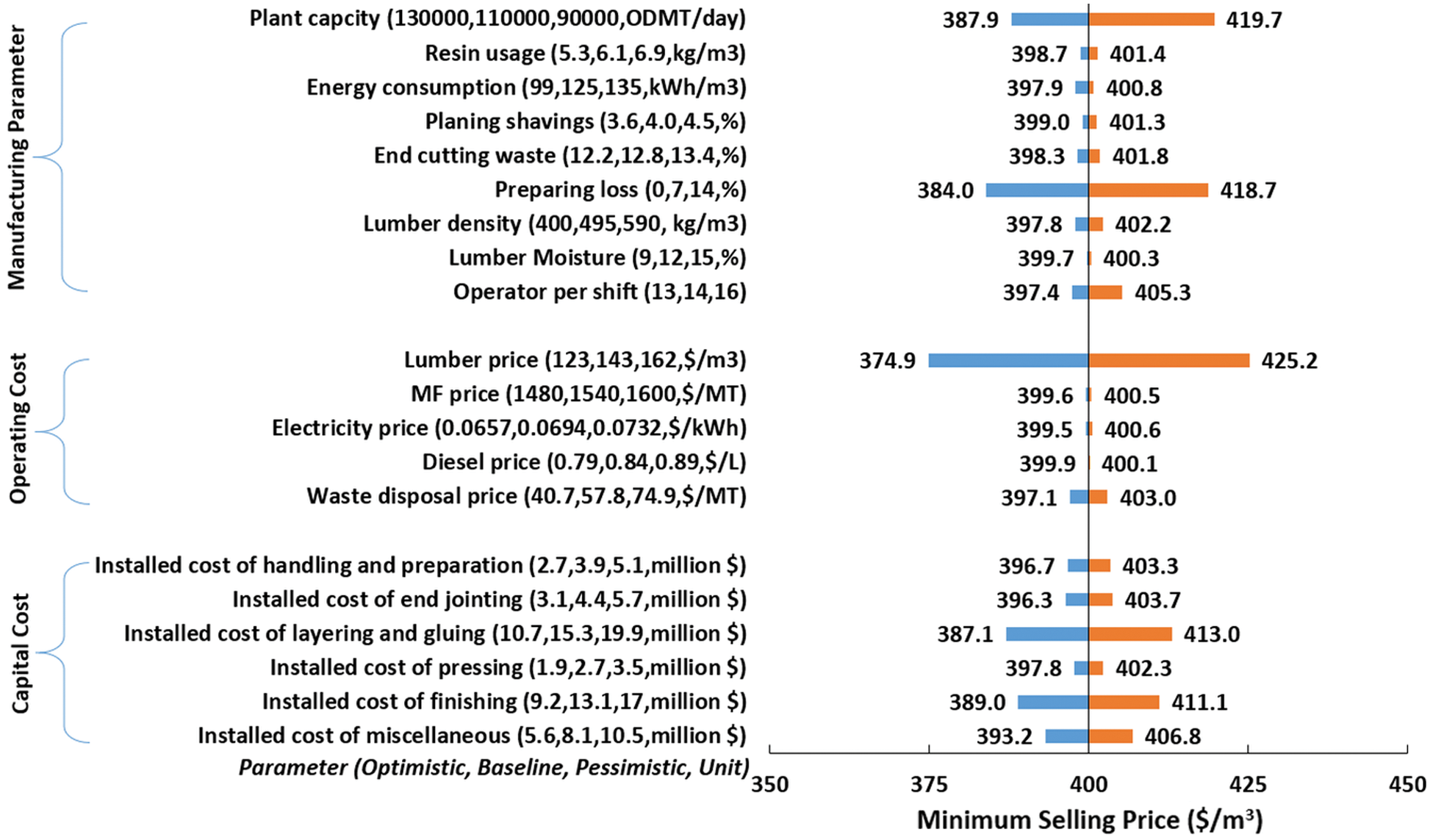
Figure 7: Sensitivity analysis results of MSP (baseline selected as the 110,000 m3/year plant)
This study explores the economic performance of producing CLT from softwood lumber in the Southern U.S. and considers the effects of variations in plant capacities, key manufacturing parameters, material and energy cost on MSP of CLT panels. The overall MSP ranges from $345 to $609/m3 across all the capacity cases from 30,000 to 150,000 m3/year. Enlarging the CLT plant capacity can significantly reduce the MSP due to the reduced capital cost and fixed operating cost per m3 CLT. The effects of variations in the feedstock, key manufacturing parameters, capital and operating cost, can cause a ±6%–9% range (P5–P95 value) in the MSP. This study also studies the transportation cost of delivering CLT from the plant to consumers supported by GIS. Three CLT demanding levels were included, 1%, 5%, and 15%. This study concludes that the transportation cost of delivering the CLT panels is much smaller (1%–8%) compared to the MSP. The transportation cost increases as the demanding level decreases or the plant capacity increases due to average longer delivering distances. Thus, when considering varied demanding levels, larger plant capacity does not necessarily generate lower delivered cost that consists of MSP and transportation cost. To identify the key drivers of the economic feasibility, this study performances a sensitivity analysis and shows that the lumber price, lumber preparing loss, plant capacity, and the installed costs of layering and gluing, finishing, and miscellaneous, are the top driving factors. This conclusion also exhibits the further direction of lowering the production cost of CLT panels.
Acknowledgement: The authors thank the support from North Carolina State University.
Funding Statement: The authors received no specific funding for this study.
Conflicts of Interest: The authors declare that they have no conflicts of interest to report regarding the present study.
1. Robertson, A. B., Lam, F. C., Cole, R. J. (2012). A comparative cradle-to-gate life cycle assessment of mid-rise office building construction alternatives: Laminated timber or reinforced concrete. Buildings, 2(3), 245–270. DOI 10.3390/buildings2030245. [Google Scholar] [CrossRef]
2. Fatahi, B., Tabatabaiefar, S. H. R. (2014). Fully nonlinear versus equivalent linear computation method for seismic analysis of midrise buildings on soft soils. International Journal of Geomechanics, 14(4), 04014016. DOI 10.1061/(ASCE)GM.1943-5622.0000354. [Google Scholar] [CrossRef]
3. Liu, Y., Guo, H., Sun, C., Chang, W. S. (2016). Assessing cross laminated timber (CLT) as an alternative material for mid-rise residential buildings in cold regions in China—A life-cycle assessment approach. Sustainability, 8(10), 1047. DOI 10.3390/su8101047. [Google Scholar] [CrossRef]
4. Brandt, K., Wilson, A., Bender, D., Dolan, J. D., Wolcott, M. P. (2019). Techno-economic analysis for manufacturing cross-laminated timber. BioResources, 14(4), 7790–7804. DOI 10.15376/biores. [Google Scholar] [CrossRef]
5. Gong, Y., Liu, F., Tian, Z., Wu, G., Ren, H. et al. (2019). Evaluation of mechanical properties of cross-laminated timber with different lay-ups using Japanese larch. Journal of Renewable Materials, 7(10), 941–956. DOI 10.32604/jrm.2019.07354. [Google Scholar] [CrossRef]
6. Chen, Z., Lu, W., Bao, Y., Zhang, J., Wang, L. et al. (2021). Numerical investigation of connection performance of timber-concrete composite slabs with inclined self-tapping screws under high temperature. Journal of Renewable Materials. DOI 10.32604/jrm.2021.015925. [Google Scholar] [CrossRef]
7. ANSI/APA PRG (2012). ANSI/APA PRG 320-2012 Standard for Performance-Rated Cross-Laminated Timber. https://www.apawood.org/ansi-apa-prg-320. [Google Scholar]
8. Wang, G. (2018). Hygrothermal performance of southern pine cross-laminated timber (Ph.D. Thesis). North Carolian State University, USA. [Google Scholar]
9. Sun, J., Niederwestberg, J., Cheng, F., Chui, Y. (2020). Frequencies prediction of laminated timber plates using ANN approach. Journal of Renewable Materials, 8(3), 319. DOI 10.32604/jrm.2020.08696. [Google Scholar] [CrossRef]
10. Yang, H., Ji, J., Tao, H., Shi, B., Hu, J. et al. (2021). Pull-out behaviour of axially loaded screwed-in threaded rods embedded in CLT elements: Experimental study. Journal of Renewable Materials, DOI 10.32604/jrm.2021.016118. [Google Scholar] [CrossRef]
11. FPInnovations (2013). CLT Handbook US Editionhttps://www.seattle.gov/dpd/cms/groups/pan/@pan/documents/web_informational/dpds021903.pdf. [Google Scholar]
12. Puettmann, M., Sinha, A., Ganguly, I. (2018). CORRIM Report-life cyle assessment of cross laminated timber produced in oregon. https://corrim.org/wp-content/uploads/2019/02/Life-Cycle-Assessment-of-Oregon-Cross-Laminated-Timber.pdf. [Google Scholar]
13. Klippel, M., Schmid, J. (2017). Design of cross-laminated timber in fire. Structural Engineering International, 27(2), 224–230. DOI 10.2749/101686617X14881932436096. [Google Scholar] [CrossRef]
14. Frangi, A., Fontana, M., Hugi, E., Jübstl, R. (2009). Experimental analysis of cross-laminated timber panels in fire. Fire Safety Journal, 44(8), 1078–1087. DOI 10.1016/j.firesaf.2009.07.007. [Google Scholar] [CrossRef]
15. Schmid, J., König, J., Köhler, J. (2010). Fire-exposed cross-laminated timber–modelling and tests. World Conference on Timber Engineering Trentino, Italy. [Google Scholar]
16. Hasburgh, L., Bourne, K., Peralta, P., Mitchell, P., Schiff, S. et al. (2016). Effect of adhesives and ply configuration on the fire performance of southern pine cross-laminated timber. World Conference on Timber Engineering Vienna, Austria. [Google Scholar]
17. Hasburgh, L., Bourne, K., Dagenais, C., Ranger, L., Roy-Poirier, A. (2016). Fire performance of mass-timber encapsulation methods and the effect of encapsulation on char rate of cross-laminated timber. World Conference on Timber Engineering Vienna, Austria. [Google Scholar]
18. Asdrubali, F., Ferracuti, B., Lombardi, L., Guattari, C., Evangelisti, L. et al. (2017). A review of structural, thermo-physical, acoustical, and environmental properties of wooden materials for building applications. Building and Environment, 114, 307–332. DOI 10.1016/j.buildenv.2016.12.033. [Google Scholar] [CrossRef]
19. Mallo, M. F. L., Espinoza, O. A. (2014). Outlook for cross-laminated timber in the United States. BioResources, 9(4), 7427–7443. DOI 10.15376/biores.9.4.7427-7443. [Google Scholar] [CrossRef]
20. Öqvist, R., Ljunggren, F., Ågren, A. (2012). On the uncertainty of building acoustic measurements–case study of a cross-laminated timber construction. Applied Acoustics, 73(9), 904–912. DOI 10.1016/j.apacoust.2012.03.012. [Google Scholar] [CrossRef]
21. Pérez, M. (2013). Acoustic design through predictive methods in cross laminated timber (CLT) panel structures in buildings. INTER-NOISE and NOISE-CON Congress and Conference Proceedings, vol. 247, pp. 5539–5547, Institute of Noise Control Engineering. Innsbruck, Austria. [Google Scholar]
22. Sharifnia, H., Hindman, D. P. (2017). Effect of manufacturing parameters on mechanical properties of southern yellow pine cross laminated timbers. Construction and Building Materials, 156, 314–320. DOI 10.1016/j.conbuildmat.2017.08.122. [Google Scholar] [CrossRef]
23. Hindman, D. P., Bouldin, J. C. (2015). Mechanical properties of southern pine cross-laminated timber. Journal of Materials in Civil Engineering, 27(9), 04014251. DOI 10.1061/(ASCE)MT.1943-5533.0001203. [Google Scholar] [CrossRef]
24. Gu, M. (2017). Strength and serviceability performances of southern yellow pine cross-laminated timber (CLT) and CLT-glulam composite beam (Ph.D. Thesis). Clemson University, USA. [Google Scholar]
25. Okabe, M., Yasumura, M., Kobayashi, K. (2014). Estimation of bending stiffness, moment carrying capacity and internal shear force of sugi CLT panels. Proceedings of World Conference on Timber Engineering, Quebec City, Canada, pp. 10–14. [Google Scholar]
26. Kramer, A., Barbosa, A. R., Sinha, A. (2014). Viability of hybrid poplar in ANSI approved cross-laminated timber applications. Journal of Materials in Civil Engineering, 26(7), 06014009. DOI 10.1061/(ASCE)MT.1943-5533.0000936. [Google Scholar] [CrossRef]
27. Gu, H., Bergman, R. (2018). Life cycle assessment and environmental building declaration for the design building at the University of Massachusetts. General Technical Report FPL-GTR-255. Madison, WI: US Department of Agriculture, Forest Service, Forest Products Laboratory. [Google Scholar]
28. Brandner, R., Flatscher, G., Ringhofer, A., Schickhofer, G., Thiel, A. (2016). Cross laminated timber (CLTOverview and development. European Journal of Wood and Wood Products, 74(3), 331–351. DOI 10.1007/s00107-015-0999-5. [Google Scholar] [CrossRef]
29. Passarelli, R. N. (2018). The environmental impact of reused CLT panels: Study of a single-storey commercial building in Japan. World Conference on Timber Engineering Seoul, Korea. [Google Scholar]
30. Dong, Y., Cui, X., Yin, X., Chen, Y., Guo, H. (2019). Assessment of energy saving potential by replacing conventional materials by cross laminated timber (CLT)—A case study of office buildings in China. Applied Sciences, 9(5), 858. DOI 10.3390/app9050858. [Google Scholar] [CrossRef]
31. Lan, K., Kelley, S. S., Prakash Nepal, Y. Y. (2020). Dynamic life cycle carbon and energy analysis for cross-laminated timber in the southeastern United States. Environmental Research Letters, 15(12), 124036. DOI 10.1088/1748-9326/abc5e6. [Google Scholar] [CrossRef]
32. Ganguly, I., Beyreuther, T., Hoffman, M., Swenson, S., Eastin, I. (2017). Forecasting the demand for cross laminated timber (CLT) in the Pacific Northwest. https://www.cintrafor.org/publications/forecasting-the-demand-for-cross-laminated-timber-clt-in-the-pacific-northwest. [Google Scholar]
33. Energias (2018). Global cross laminated timber (CLT) market outlook, trend and opportunity analysis, competitive insights, actionable segmentation & forecast 2024. https://www.energiasmarketresearch.com/global-cross-laminated-timber-market-outlook/. [Google Scholar]
34. Beck Group (2018). Mass timber market analysis. https://www.oregon.gov/ODF/Documents/ForestBenefits/Beck-mass-timber-market-analysis-report.pdf. [Google Scholar]
35. APA (2020). CLT manufacturers. https://www.apawood.org/cross-laminated-timber#:~:text=CLTManufacturers,LLCKalesnikoffMassTimber%2CInc. [Google Scholar]
36. Espinoza, O., Buehlmann, U., Laguarda, M., Trujillo, V. R. (2016). Identification of research areas to advance the adoption of cross-laminated timber in North America. BioProducts Business, 1(5), 60–72. DOI 10.22382/bpb-2016-005. [Google Scholar] [CrossRef]
37. Albee, R. R. (2019). Global overview of the cross-laminated timber industry (Master Thesis). Oregon State University, USA. [Google Scholar]
38. Lan, K., Park, S., Kelley, S. S., English, B. C., Yu, T. H. E. et al. (2020). Impacts of uncertain feedstock quality on the economic feasibility of fast pyrolysis biorefineries with blended feedstocks and decentralized preprocessing sites in the southeastern United States. GCB Bioenergy, 12(11), 1014–1029. DOI 10.1111/gcbb.12752. [Google Scholar] [CrossRef]
39. Wright, M. M., Daugaard, D. E., Satrio, J. A., Brown, R. C. (2010). Techno-economic analysis of biomass fast pyrolysis to transportation fuels. Fuel, 89, S2–S10. DOI 10.1016/j.fuel.2010.07.029. [Google Scholar] [CrossRef]
40. Sahoo, K., Bilek, E. T., Mani, S. (2018). Techno-economic and environmental assessments of storing woodchips and pellets for bioenergy applications. Renewable and Sustainable Energy Reviews, 98, 27–39. DOI 10.1016/j.rser.2018.08.055. [Google Scholar] [CrossRef]
41. Bédard, P., Fournier, F., Gagnon, S., Gingras, A., Lavoie, V. et al. (2010). Manufacturing cross-laminated timber (CLT) technological and economic analysis. https://library.fpinnovations.ca/en/permalink/fpipub39323. [Google Scholar]
42. Shahrukh, H., Oyedun, A. O., Kumar, A., Ghiasi, B., Kumar, L. et al. (2016). Techno-economic assessment of pellets produced from steam pretreated biomass feedstock. Biomass and Bioenergy, 87, 131–143. DOI 10.1016/j.biombioe.2016.03.001. [Google Scholar] [CrossRef]
43. Sahoo, K., Bilek, E., Bergman, R., Mani, S. (2019). Techno-economic analysis of producing solid biofuels and biochar from forest residues using portable systems. Applied Energy, 235, 578–590. DOI 10.1016/j.apenergy.2018.10.076. [Google Scholar] [CrossRef]
44. Swanson, R. M., Platon, A., Satrio, J. A., Brown, R. C. (2010). Techno-economic analysis of biomass-to-liquids production based on gasification. Fuel, 89, S11–S19. DOI 10.1016/j.fuel.2010.07.027. [Google Scholar] [CrossRef]
45. Humbird, D., Davis, R., Tao, L., Kinchin, C., Hsu, D. et al. (2011). Process design and economics for biochemical conversion of lignocellulosic biomass to ethanol: Dilute-acid pretreatment and enzymatic hydrolysis of corn stover (No. NREL/TP-5100-47764), National Renewable Energy Laboratory (NRELGolden, USA. [Google Scholar]
46. ANSI/APA (2019). ANSI/APA PRG 320-2019 Standard for Performance-Rated Cross-Laminated Timber. https://www.apawood.org/ansi-apa-prg-320. [Google Scholar]
47. Muszynski, L. (2017). Effective bonding parameters for hybrid cross-laminated timber (CLT) (Master Thesis). Oregon State University, USA. [Google Scholar]
48. Chen, C. X., Pierobon, F., Ganguly, I. (2019). Life cycle assessment (LCA) of cross-laminated timber (CLT) produced in western Washington: The role of logistics and wood species mix. Sustainability, 11(5), 1278. DOI 10.3390/su11051278. [Google Scholar] [CrossRef]
49. ASMI (2013). A life cycle assessment of cross-laminated timber produced in Canada. http://www.athenasmi.org/resources/publications/. [Google Scholar]
50. Popovski, M., Gavric, I. (2016). Performance of a 2-story CLT house subjected to lateral loads. Journal of Structural Engineering, 142(4), E4015006. DOI 10.1061/(ASCE)ST.1943-541X.0001315. [Google Scholar] [CrossRef]
51. Patterson, D. W., Doruska, P. F., Posey, T. (2004). Weight and bulk density of loblolly pine plywood logs in southeast Arkansas. Forest Products Journal, 54(12), 145–149. [Google Scholar]
52. Patterson, D. W., Clark III, A. (1988). Bulk density of southern pine logs. Forest Products Journal, 38, 36–40. [Google Scholar]
53. Miles, P. D., Smith, W. B. (2009). Specific gravity and other properties of wood and bark for 156 tree species found in North America, vol. 38. US Department of Agriculture, Forest Service, Northern Research Station. [Google Scholar]
54. Dutta, A., Sahir, A. H., Tan, E., Humbird, D., Snowden-Swan, L. J. et al. (2015). Process design and economics for the conversion of lignocellulosic biomass to hydrocarbon fuels: Thermochemical research pathways with in Situ and ex Situ upgrading of fast pyrolyss vapors (No. PNNL-23823), Pacific Northwest National Laboratory (PNNLRichland, USA. [Google Scholar]
55. Kazi, F. K., Fortman, J., Anex, R., Kothandaraman, G., Hsu, D. et al. (2010). Techno-economic analysis of biochemical scenarios for production of cellulosic ethanol (No. NREL/TP-6A2-46588). National Renewable Energy Laboratory (NRELGolden, USA. [Google Scholar]
56. Ou, L., Kim, H., Kelley, S., Park, S. (2018). Impacts of feedstock properties on the process economics of fast-pyrolysis biorefineries. Biofuels, Bioproducts and Biorefining, 12(3), 442–452. DOI 10.1002/bbb.1860. [Google Scholar] [CrossRef]
57. Jones, S. B., Meyer, P. A., Snowden-Swan, L. J., Padmaperuma, A. B., Tan, E. et al. (2013). Process design and economics for the conversion of lignocellulosic biomass to hydrocarbon fuels: Fast pyrolysis and hydrotreating bio-oil pathway (No. PNNL-23053; NREL/TP-5100-61178). Pacific Northwest National Laboratory (PNNLRichland, USA. [Google Scholar]
58. Beaves, R. G. (1988). Net present value and rate of return: Implicit and explicit reinvestment assumptions. The Engineering Economist, 33(4), 275–302. DOI 10.1080/00137918808966958. [Google Scholar] [CrossRef]
59. Osborne, M. J. (2010). A resolution to the NPV–IRR debate? The Quarterly Review of Economics and Finance, 50(2), 234–239. DOI 10.1016/j.qref.2010.01.002. [Google Scholar] [CrossRef]
60. Chemical Engineering Magazine (2019). Plant cost index. https://www.bing.com/search?q=Chemical+Engineering+Magazine.+(2015).+Plant+Cost+Index.&cvid=fe1d10de53d04969b721e43428d8e2a8&aqs=edge.69i57.337j0j9&FORM=ANAB01&PC=LCTS. [Google Scholar]
61. Peters, M. S., Timmerhaus, K. D., West, R. E. (2003). Plant design and economics for chemical engineers, vol. 4. New York: McGraw-Hill. [Google Scholar]
62. Tao, L., Markham, J. N., Haq, Z., Biddy, M. J. (2017). Techno-economic analysis for upgrading the biomass-derived ethanol-to-jet blendstocks. Green Chemistry, 19(4), 1082–1101. DOI 10.1039/C6GC02800D. [Google Scholar] [CrossRef]
63. Pirraglia, A., Gonzalez, R., Saloni, D., Denig, J. (2013). Technical and economic assessment for the production of torrefied ligno-cellulosic biomass pellets in the US. Energy Conversion and Management, 66, 153–164. DOI 10.1016/j.enconman.2012.09.024. [Google Scholar] [CrossRef]
64. Turner, T. A., Harper, L. T., Warrior, N. A., Rudd, C. D. (2008). Low-cost carbon-fibre-based automotive body panel systems: A performance and manufacturing cost comparison. Proceedings of the Institution of Mechanical Engineers, Part D: Journal of Automobile Engineering, 222(1), 53–63. DOI 10.1243/09544070JAUTO406. [Google Scholar] [CrossRef]
65. Alibaba (2020). Edge trimming machine. https://www.alibaba.com/product-detail/45-degree-edge-banding-machinechina_62070871941.html?spm=a2700.galleryofferlist.normal_offer.d_title.4b02eb8eAsmedw&s=p&fullFirstScreen=true. [Google Scholar]
66. Trading Economics (2019). Lumber price. https://tradingeconomics.com/commodity/lumber. [Google Scholar]
67. Federal Reserve Bank of St. Louis (2019). Producer price index by commodity: Lumber and wood products: Softwood lumber. https://fred.stlouisfed.org/series/WPU0811. [Google Scholar]
68. Alibaba.com (2019). Melamine formaldehyde price. https://www.alibaba.com/showroom/melamine-formaldehyde-resins.html. [Google Scholar]
69. US EIA (2019). Average price of electricity to ultimate customers by End-use sector. https://www.eia.gov/electricity/monthly/epm_table_grapher.php?t=epmt_5_6_a. [Google Scholar]
70. US EIA (2019). Weekly retail gasoline and diesel prices. https://www.eia.gov/dnav/pet/pet_pri_gnd_dcus_nus_m.htm. [Google Scholar]
71. US EPA (2014). Municipal solid waste landfills economic impact analysis for the proposed New subpart to the New source performance standards. https://www3.epa.gov/ttnecas1/docs/eia_ip/solid-waste_eia_nsps_proposal_07-2014.pdf. [Google Scholar]
72. Bureau of Labor Statistics (2020). Producer price indexes. https://www.bls.gov/pPI/. [Google Scholar]
73. Bureau of Labor Statistics (2020). Labor index by bureau of labor statistics. https://data.bls.gov/cgi-bin/srgate. [Google Scholar]
74. United States Census Bureau (2019). Building permits survey. https://www.census.gov/construction/bps/. [Google Scholar]
75. US EIA (2016). 2012 commercial buildings energy consumption survey (CBECS) survey data. https://www.eia.gov/consumption/commercial/data/2012/. [Google Scholar]
76. Chen, Y. (2012). Comparison of environmental performance of a five-storey building built with cross-laminated timber and concrete. Sustainable building science program. University of British Columbia-Department of Wood Science, Vancouver, BC, Canada. [Google Scholar]
77. Pierobon, F., Huang, M., Simonen, K., Ganguly, I. (2019). Environmental benefits of using hybrid CLT structure in midrise non-residential construction: An LCA based comparative case study in the US pacific northwest. Journal of Building Engineering, 26, 100862. DOI 10.1016/j.jobe.2019.100862. [Google Scholar] [CrossRef]
78. ESRI (2020). ArcGIS 10.6. https://desktop.arcgis.com/en/arcmap/. [Google Scholar]
79. US Census Bureau Department of Commerce (2018). TIGER/line shapefile, series information for the primary and secondary roads state-based shapefile. https://catalog.data.gov/dataset/tiger-line-shapefile-2018-series-information-for-the-primary-and-secondary-roads-state-based-sh. [Google Scholar]
80. US Census Bureau Department of Commerce (2009). 2009 TIGER/Line shapefiles technical documentation. https://www2.census.gov/geo/pdfs/maps-data/data/tiger/tgrshp2009/TGRSHP09AF.pdf. [Google Scholar]
81. Skszek, S. L. (2004). Actual speeds on the roads compared to the posted limits. https://safety.fhwa.dot.gov/speedmgt/ref_mats/fhwasa09028/resources/actualspeedsonroadtopostedlimits.pdf. [Google Scholar]
82. Murray, D., Glidewell, S. (2019). An analysis of the operational costs of trucking: 2019 update. https://truckingresearch.org/wp-content/uploads/2019/11/ATRI-Operational-Costs-of-Trucking-2019-1.pdf. [Google Scholar]
83. Wells, L. A., Chung, W., Anderson, N. M., Hogland, J. S. (2016). Spatial and temporal quantification of forest residue volumes and delivered costs. Canadian Journal of Forest Research, 46(6), 832–843. DOI 10.1139/cjfr-2015-0451. [Google Scholar] [CrossRef]
84. US EIA (2020). U.S. No 2 diesel retail prices. https://www.eia.gov/dnav/pet/hist/LeafHandler.ashx?n=PET&s=EMD_EPD2D_PTE_NUS_DPG&f=M. [Google Scholar]
Appendix A. Supplementary tables
Appendix B. Supplementary figures
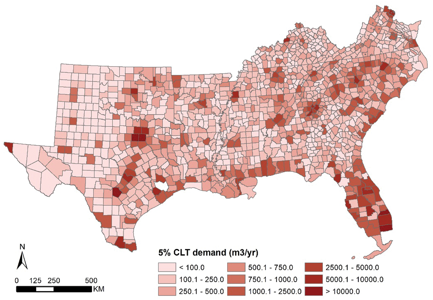
Figure S1: County-level CLT demanding results at 5% demanding level in the southern U.S.
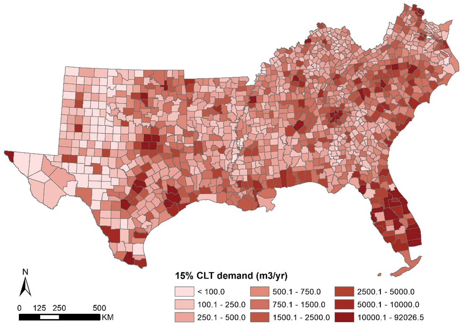
Figure S2: County-level CLT demanding results at 15% demanding level in the southern U.S.
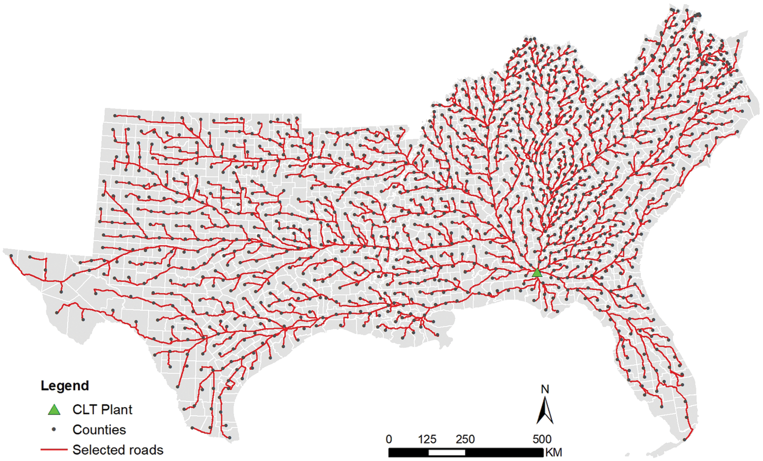
Figure S3: County-level route analysis of transportation in the southern U.S.
 | This work is licensed under a Creative Commons Attribution 4.0 International License, which permits unrestricted use, distribution, and reproduction in any medium, provided the original work is properly cited. |