| Journal of Renewable Materials |
DOI: 10.32604/jrm.2022.022300
ARTICLE
Research on Rosewood Micro Image Classification Method Based on Feature Fusion and ELM
1School of Information and Electrical Engineering, Shandong Jianzhu University, Jinan, 250101, China
2School of Architecture and Urban Planning, Shandong Jianzhu University, Jinan, 250101, China
*Corresponding Author: Yisheng Gao. Email: gao_sdjz@126.com
Received: 03 March 2022; Accepted: 02 April 2022
Abstract: Rosewood is a kind of high-quality and precious wood in China. The correct identification of rosewood species is of great significance to the import and export trade and species identification of furniture materials. In this paper, micro CT was used to obtain the micro images of cross sections, radial sections and tangential sections of 24 kinds of rosewood, and the data sets were constructed. PCA method was used to reduce the dimension of four features including logical binary pattern, local configuration pattern, rotation invariant LBP, uniform LBP. These four features and one feature not reducing dimension (rotation invariant uniform LBP) was fused with Gray Level Co-Occurrence Matrix and Tamura features, respectively, a total of five fused features LBP+GLCM+Tamura, LCP+GLCM+Tamura,
Keywords: Rosewood; micro CT; feature fusion; ELM; BP neural network
Wood, with the characteristics of ecological and environment-friendly, is an anisotropic biomass material. There are many kinds of wood, and there are great differences among different families and genera. The characteristics of similarity and difference appear in different wood in a family and genus. The category of wood is difficult to identify through macro structure, such as color, material and texture [1,2]. Experienced experts are needed for wood identification, according to the distribution of wood microstructure, such as vessel pores, wood rays and axial parenchyma in cross sections, radial sections and tangential sections [3–5]. Although this identification method is very effective, the standard of wood scientific knowledge and skills of personnel is highly required in order to realize wood classification [6,7]. Comparing with traditional anatomical methods, a micro CT was used to collect the images of cross sections, radial sections and tangential sections of wood, and thousands of wood images were generated efficiently in a short time.
Some specific features of the micro images of wood were extracted for feature fusion, which were combined with ELM (Extreme Learning Machine) classifier to realize the rapid recognition of wood through cross section, radial section and tangential section. The method of feature fusion could combine the advantages of different features to improve the classification accuracy [8,9]. Ahmad et al. [10] applied the method of deep feature fusion to waste classification to obtain high classification accuracy. Zhao et al. [11] fused the characteristics of wood texture and spectrum, and BP neural network was used for wood classification, with a correct rate of 90%. After the fusion of texture and near-infrared spectral features, SVM (Support Vector Machine) was adopted by Wang et al. [12]. The accuracy could reach 100% without interference, and the classification accuracy was better than the traditional algorithm in the case of image distortion. The above feature fusion methods were based on spectral images, but a variety of texture features were extracted, fused and classified from micro images in this paper.
ELM, as a single hidden layer feedforward neural network algorithm, was widely used in image classification [13,14], data label classification [15], fingerprint classification [16] and other fields, with good learning efficiency and generalization performance. Xiao et al. [17] classified 180 samples of 6 kinds of construction waste obtained by hyperspectral technology, and the accuracy of ELM can reach 100%, showing a strong classification ability. Yang et al. [18] extracted the data characteristics of wood defects and used the ELM for classification. The accuracy rate reached 96.72% within 187 ms. Some researchers [19,20] used ELM to classify the spectral images of wood, and the classification accuracy reached more than 97%. Xiang et al. [21] proposed a wood classification algorithm based on LBP-DEELM (Local Binary Pattern-DE-ELM) model, which has better classification accuracy than BP neural network and SVM algorithm.
In this paper, the PCA (Principal Component Analysis) method was used to reduce the dimension of four features logical binary pattern (LBP), local configuration pattern (LCP), rotation invariant LBP (
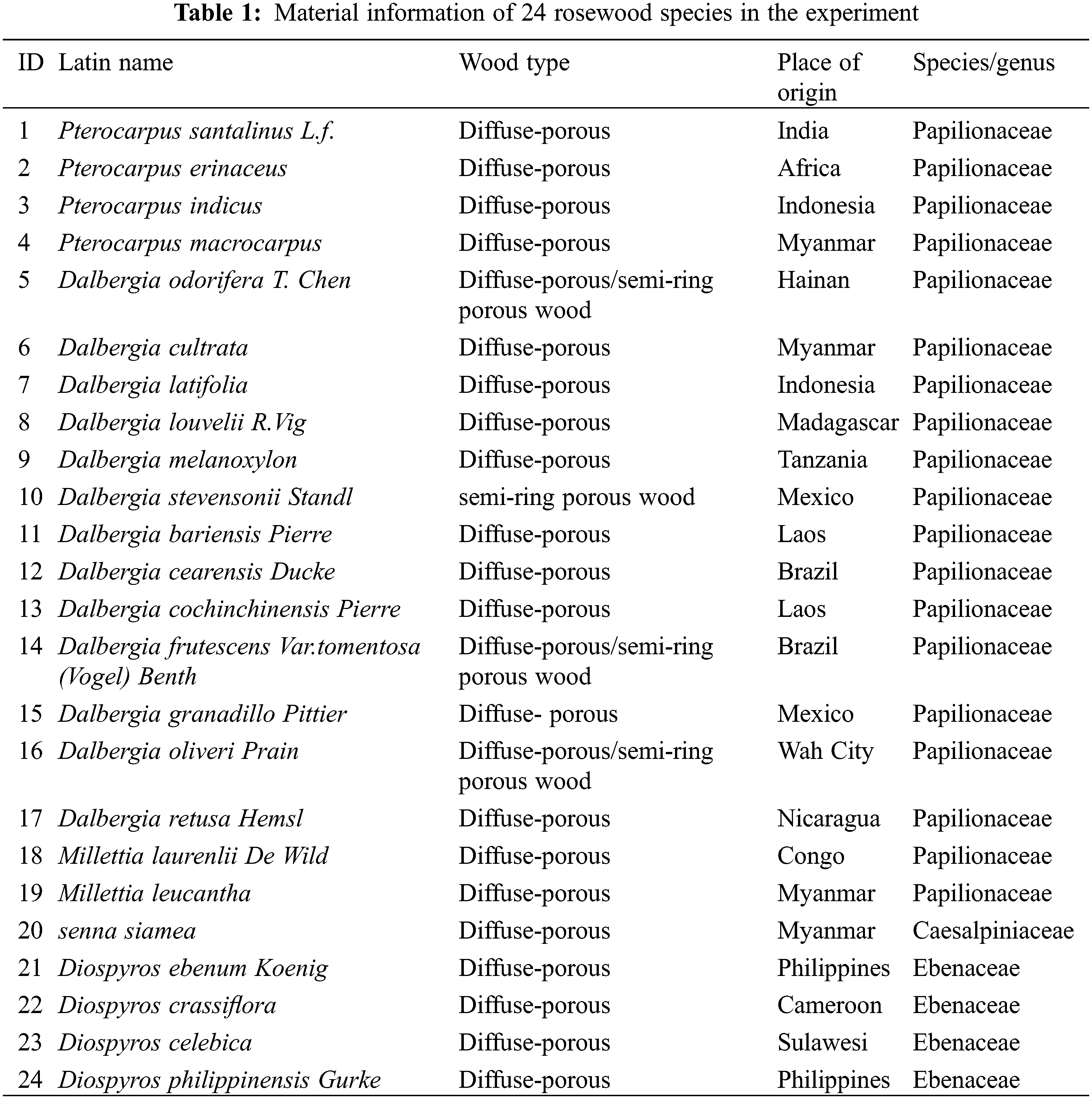
According to the rosewood standard formulated by China in 2017, rosewood is divided into 29 species. This paper takes 24 species of rosewood as the research objects from 3 families (Papilionaceae, Ebenaceae, Caesalpiniaceae) and 5 genera (Pterocarpus, Dalbergia, Millettia, Senna, Diospyros). Among them, Pterocarpus includes 4 species: Pterocarpus santalinus L.f., Pterocarpus erinaceus, Pterocarpus indicus and Pterocarpus macrocarpus. Dalbergia includes 13 species: Dalbergia odorifera T. Chen, Dalbergia cultrata, Dalbergia latifolia, Dalbergia louvelii R.Vig, Dalbergia melanoxylon, Dalbergia stevensonii Standl, Dalbergia bariensis Pierre, Dalbergia cearensis Ducke, Dalbergia cochinchinensis Pierre, Dalbergia frutescens Var.tomentosa (Vogel) Benth, Dalbergia granadillo Pittier, Dalbergia oliveri Prain, Dalbergia retusa Hemsl. Millettia includes 2 species: Millettia laurenlii De Wild, Millettia leucantha. Senna includes 1 species: senna siamea. Diospyros includes 4 species: Diospyros sp., Diospyros crassiflora, Diospyros celebica, Diospyros sp. The Latin names of 24 kinds of rosewood, the types of vessel pores, family names and origin information were given in Table 1. The experimental materials were taken from the Specimens Museum of the Shandong Jianzhu University (Jinan, China).
The wood was prepared into small specimens with a size of 5 mm × 5 mm × 20 mm and scanned by micro-CT (SKYSCAN1272). The specimens and equipment are shown in Fig. 1. The specimen was put into the micro-CT and fixed well. The scanning parameters were set to 50 kV, 200 mA, and the scanning resolution was 2 μm. The height of the specimen was set to about 10 mm, and the scanning time of each specimen was about 100 min. After the scanned specimens were reconstructed, images of cross sections, radial sections and tangential sections of wood could be obtained.
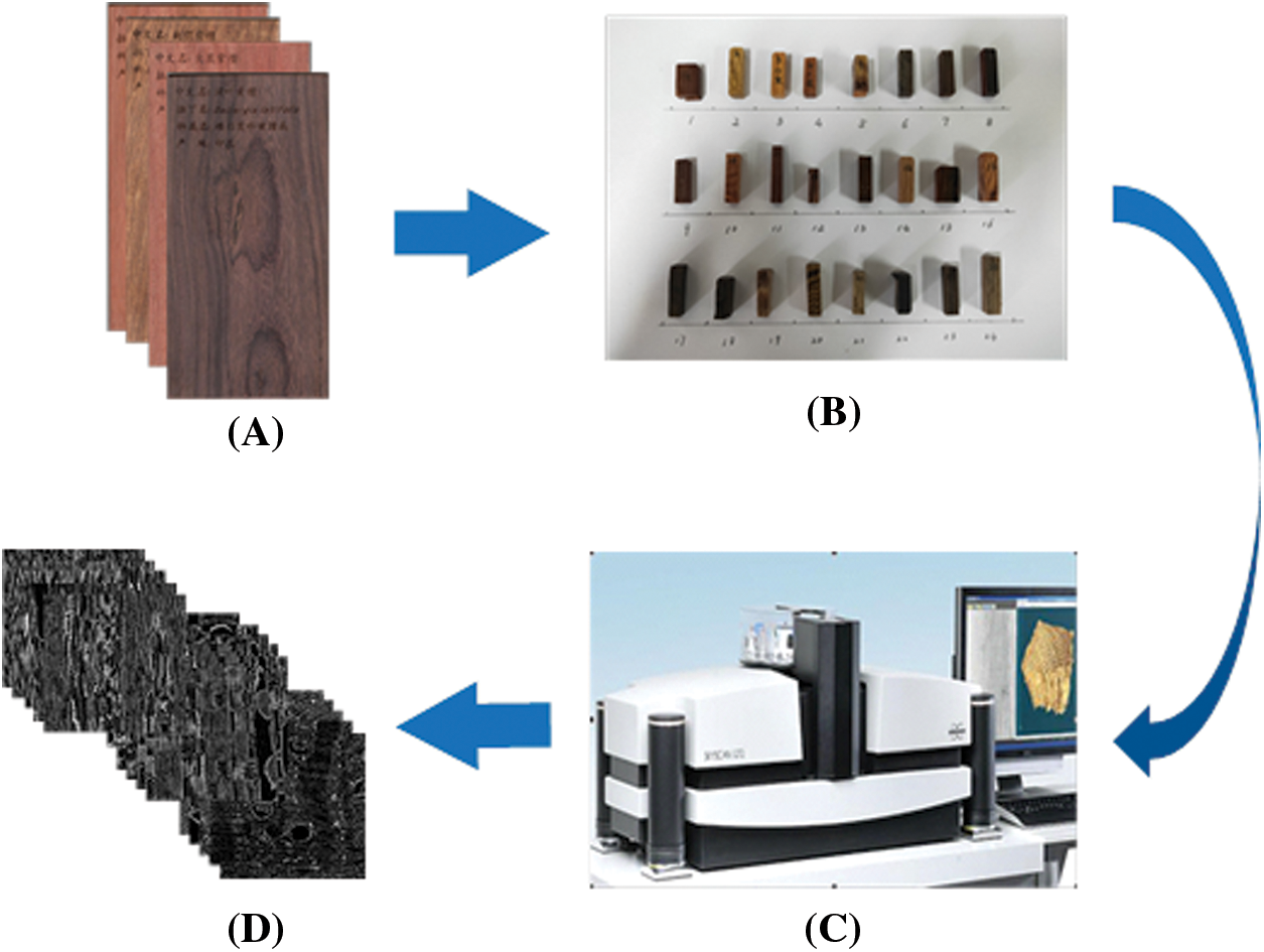
Figure 1: Acquisition of micro images. (A) is original samples; (B) is scanning specimens; (C) is scanning equipment; (D) are micro images
There were 3000 images collected from each specimen, including 1000 images from the cross sections, 1000 images from the radial sections and 1000 images from the tangential sections. 100 images were randomly selected from each section and then randomly cut into sub-images with the size of 500 px × 500 px, which were used to construct the data set of wood three sections. Ultimately, 7200 micro images of wood were obtained, which came from 2400 images of each tangential section, radial sections section and tangential section of 24 tree species, for the training of ELM and BP neural network.
The logical binary pattern (LBP), uniform LBP (
3.1.1 LBP (Logical Binary Pattern)
LBP is a kind of operator to describe texture features, which was first proposed by Ojala et al. [22]. The original LBP operator is defined as a 3 × 3 window, taking the center pixel of the window as the threshold and comparing it with the gray value of the 8 adjacent pixels. If the surrounding pixel is larger than the center pixel, it is marked as 1; otherwise, it is marked as 0. Eight points produce an 8-bit unsigned number, the LBP value of the form, which represents the texture information for the expected region. By replacing the square neighborhood with a circular neighborhood, the 3 × 3 window of the classical LBP operator is extended to an arbitrary range of radius R. Circular LBP operator was proposed by Ojala et al. [23] in 2002. The mathematical expression of circular LBP operator is:
Uniform pattern is defined as LBP binary pattern, there are two jumps from 0 to 1 or from 1 to 0 at most. For example, 00001000 (two jumps, 0-1,1-0) and 00110000 (0-1,1-0) are uniform patterns. The formula of uniform pattern is as follows:
When U ≤ 2 is in uniform pattern, it is expressed by
In order to make the LBP operator rotation invariant, Ojala et al. [23] proposed the concept of Rotation Invariant LBP. By rotating clockwise for one revolution according to the number of adjacent points, different binary codes can be obtained in the circular region. The rotation invariant property is described by the LBP value of the region, which is the minimum value in binary coding. The mathematical expressions are as follows:
ROR(x, i) is a function used to rotate, performing a circular bit-wise right shift on the x-bit binary number by i times.
3.1.4 Rotation Invariant Uniform LBP
Combining the rotation invariant LBP with the uniform pattern to obtain the Rotation invariant uniform LBP, which has better effect. It is represented by symbols
3.1.5 LCP (Local Configuration Pattern)
LCP model is used to describe the texture features of images. The algorithm consists of two parts: the traditional LBP texture feature and the microscopic structure feature. By combining the above two features, the image information expression of LCP model is more detailed [24]. LBP features are calculated by comparing the gray values of a pixel with those of neighboring points. The structure of the LCP is illustrated in Fig. 2.
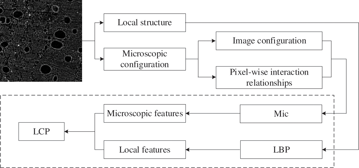
Figure 2: A structure for feature extraction of LCP
In addition to LBP and its deformation features, GLCM (Gray Level Co-Occurrence Matrix) and Tamura features were extracted, respectively. GLCM feature is a common method to describe texture by researching the spatial correlation characteristics of image gray scale. Inspired by human visual perception and psychological research, six Tamura texture features have been proposed. Roughness, contrast, directivity, linearity, regularity and roughness are used to extract texture features of micro images in this paper.
3.2 PCA Principle and Feature Dimension Reduction
PCA (Principal Component Analysis) is a method to build a new feature set by combining the existing features to remove redundant features and reduce dimension. On the premise of better representing the original feature data, PCA essentially projects the sample data in high-dimensional space to low-dimensional space through linear transformation [25,26].
Assuming that there are N training images with the size of m × n and the dimension of M = m × n, the i-th image is represented by one-dimensional vector xi, and N images can be represented as a training set X, as shown in formula (6):
The mean value of training samples
The difference between the training sample and the sample mean
Obviously, the covariance matrix S is a real symmetric matrix, and the existence of matrix u makes S similar to the diagonal matrix, as shown in (9):
Among them
For features (LBP, LCP,
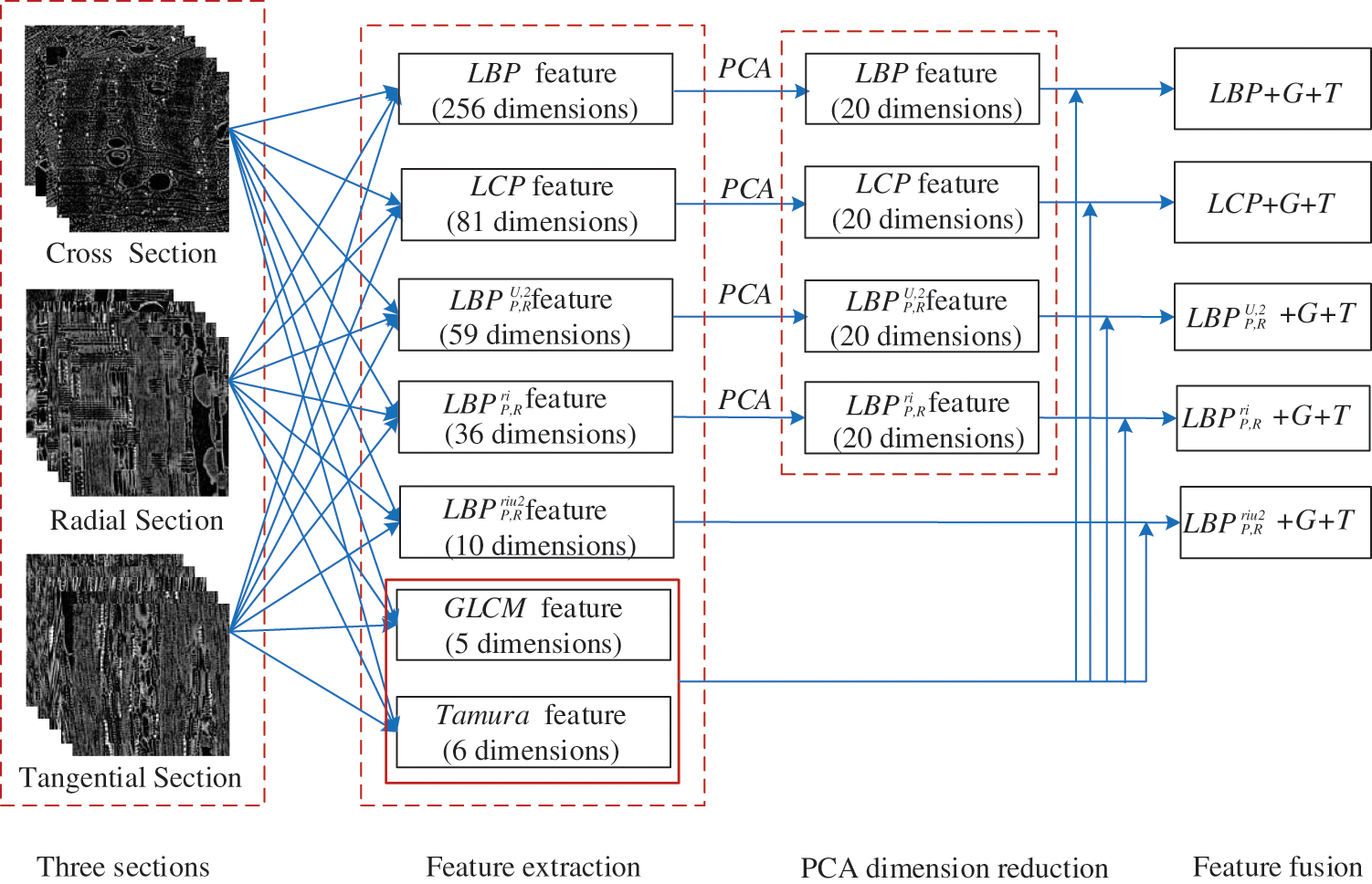
Figure 3: PCA reduction dimension and feature fusion
In view of the cross sections, radial sections and tangential sections of each species in 24 kinds of rosewood, five feature fusion methods (LBP+G+T, LCP+G+T,
ELM is a new single hidden layer feedforward neural network proposed by Huang [27]. This algorithm does not require complex iterative calculation, which is straightforward to select parameters, rapid learning speed and good generalization performance [17]. By setting the number of hidden layer nodes, the network can generate a unique optimal solution through random input weights and hidden layer bias. For the five fused features, the number of nodes in the hidden layer is set as 50 in this paper.
The BP neural network consists of three layers: the input layer, the hidden layer and the output layer. The hyperbolic tangent function tanh was used as the transfer function from the input layer to the hidden layer, and the purelin function was used as the transfer function from the hidden layer to the output layer. The training times were 1000 and the learning rate was 0.01, the error rate of the training target was 0.00001, the momentum parameter was 0.01, and the minimum performance gradient was 1e−6.
The classification results of five fused features by ELM and BP neural network were given in this paper, and the classification performance of the two classifiers in cross sections, radial sections and tangential sections were compared.
Five fused features (LBP+G+T, LCP+G+T,
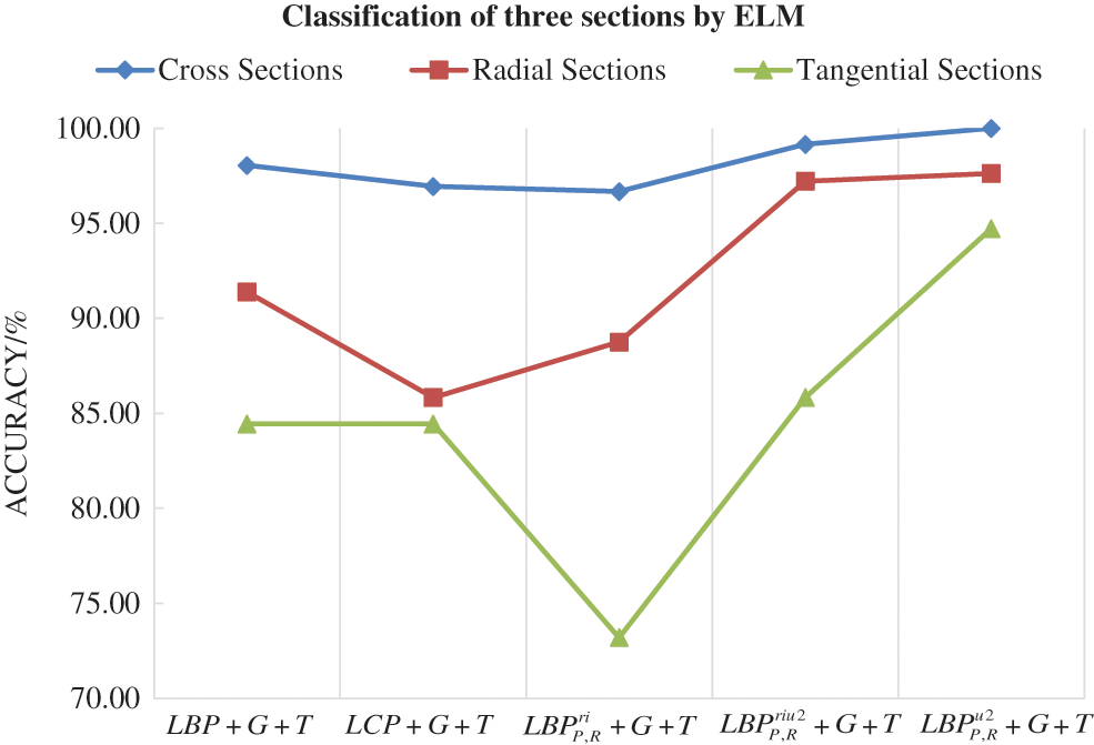
Figure 4: Classification of three sections by ELM
4.2 BP Neural Network Classification
Five fused features (LBP+G+T, LCP+G+T,
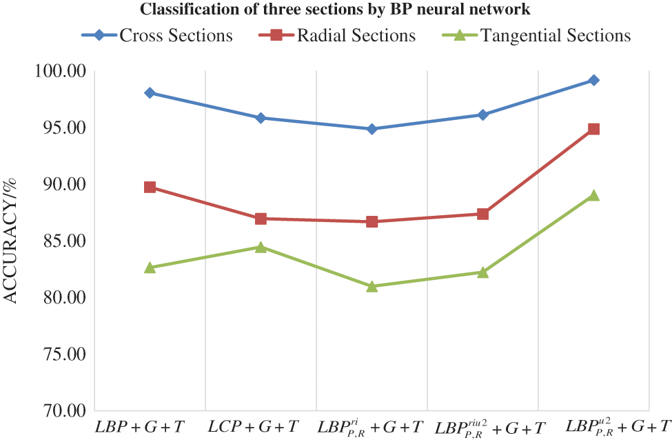
Figure 5: Classification of three sections by BP neural network
4.3 Comparison of ELM and BP Neural Network Results
In order to evaluate the performance of the two classifiers, the classification results of ELM and BP neural network in three sections are compared, as shown in Fig. 6. In the classification of cross sections as shown in (A), the classification accuracy of ELM is higher than that of BP neural network. In the classification of radial sections as shown in (B), except for LCP+G+T features, the classification accuracy of other four features ELM is higher than that of BP neural network. In the classification of tangential sections as shown in (C), except for
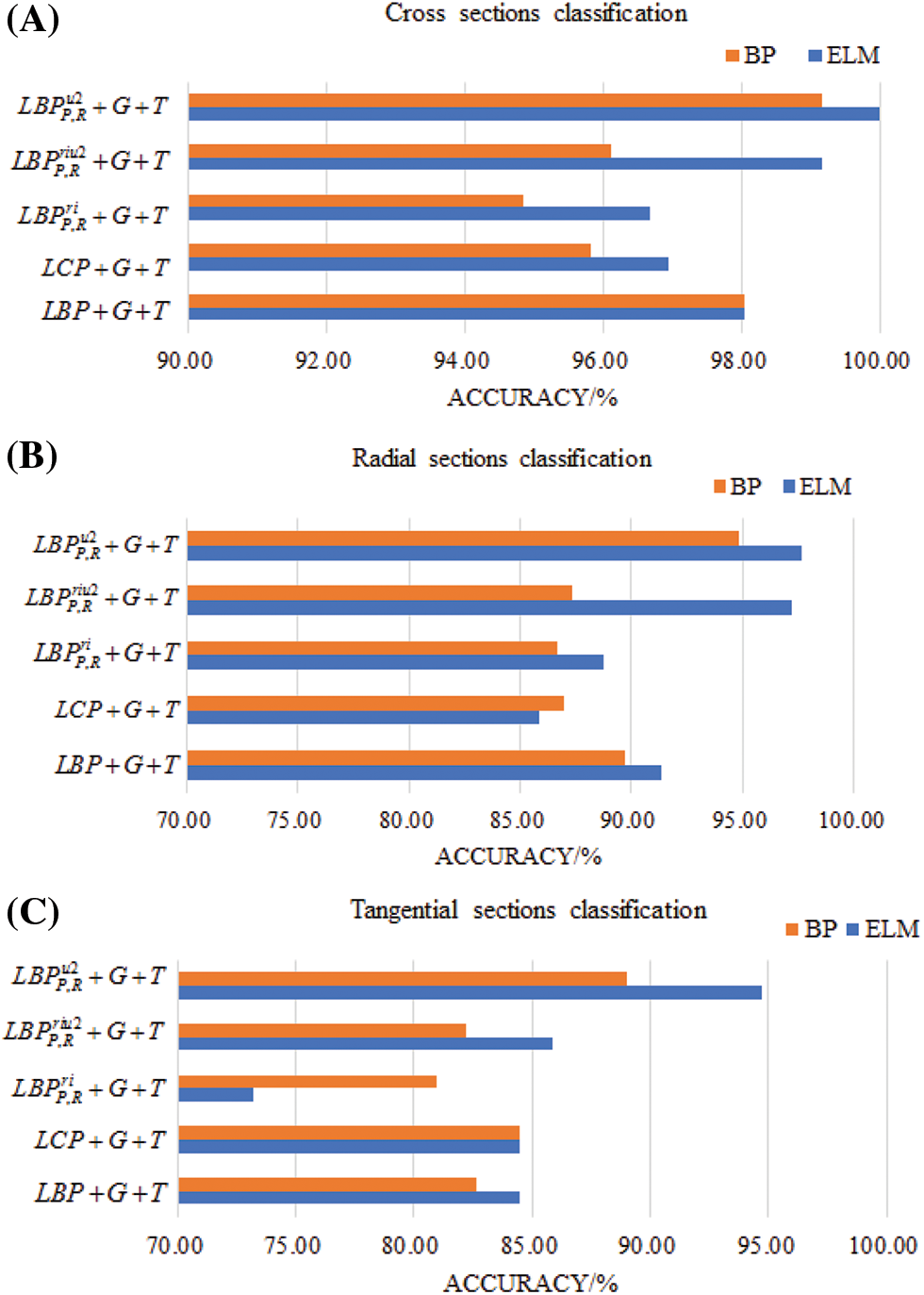
Figure 6: Compared the classification results of ELM and BP neural network in three sections, (A) is Cross sections classification accuracy; (B) is radial sections classification accuracy; (C) is tangential sections classification accuracy
As can be seen from Table 2, among the five fusion features classified by ELM and BP neural network,
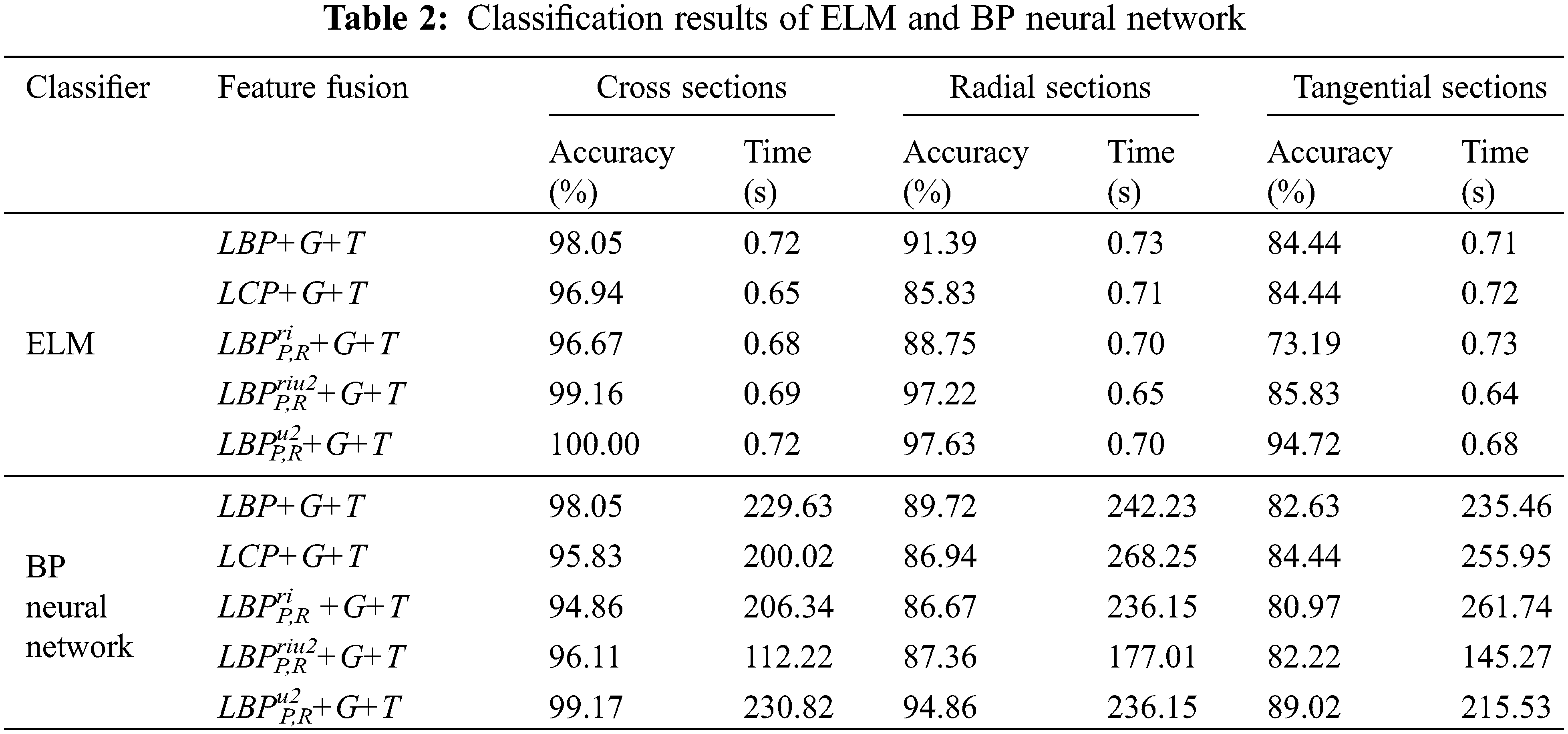
1. In the classification of three sections using five fused texture features (LBP+G+T, LCP+G+T,
2. Among the five texture feature fusion methods,
Funding Statement: The Natural Science Foundation of Shandong Province, China (Grant No. ZR2020QC174). The Application of Computed Tomography (CT) Scanning Technology to Damage Detection of Timber Frames of Architectural Heritage. The Taishan Scholar Project of Shandong Province, China (Grant No. 2015162).
Conflicts of Interest: The authors declare that they have no conflicts of interest to report regarding the present study.
1. Barmpoutis, P., Dimitropoulos, K., Barboutis, I., Grammalidis, N., Lefakis, P. (2017). Wood species recognition through multidimensional texture analysis. Computers and Electronics in Agriculture, 144(4), 241–248. DOI 10.1016/j.compag.2017.12.011. [Google Scholar] [CrossRef]
2. Jahanbanifard, M., Beckers, V., Koch, G., Beeckman, H., Gravendeel, B. et al. (2020). Description and evolution of wood anatomical characters in the ebony wood genus Diospyros and its close relatives (EbenaceaeA first step towards combatting illegal logging. IAWA Journal, 41(4), 577–619. DOI 10.1163/22941932-bja10040. [Google Scholar] [CrossRef]
3. IAWA Committee (2004). IAWA list of microscopic features for softwood identification. IAWA Journal, 25(1), 1–70. DOI 10.1163/22941932-90000349. [Google Scholar] [CrossRef]
4. Wheeler, E. A. (1989). IAWA list of microscopic features for hardwood identification. IAWA Journal, 10(3), 219–332. [Google Scholar]
5. Helmling, S., Olbrich, A., Heinz, I., Koch, G. (2018). Atlas of vessel elements. IAWA Journal, 39(3), 249–352. DOI 10.1163/22941932-20180202. [Google Scholar] [CrossRef]
6. Kamal, K., Qayyum, R., Mathavan, S., Zafar, T. (2017). Wood defects classification using laws texture energy measures and supervised learning approach. Advanced Engineering Informatics, 34, 125–135. DOI 10.1016/j.aei.2017.09.007. [Google Scholar] [CrossRef]
7. Stepanova, A. V., Vasilyeva, N. A. (2021). Wood identification of an ancient Greek coffin from the Bosporan Kingdom. IAWA Journal, 42(2), 209–215. DOI 10.1163/22941932-bja10048. [Google Scholar] [CrossRef]
8. Yusof, R., Rosli, N. R., Khalid, M. (2010). Using gabor filters as image multiplier for tropical wood species recognition system. IEEE 2010 12th International Conference on Computer Modelling and Simulation, pp. 289–294. Cambridge, UK. [Google Scholar]
9. Yan, M. Z., Wang, H. Y., Wu, Y. Y., Cao, X. X., Xu, H. L. (2021). Detection of chlorophyll content of Epipremnum aureum based on fusion of spectrum and texture features. Journal of Nanjing Agricultural University, 44(3), 568–575. DOI 10.7685/jnau.2020060131. [Google Scholar] [CrossRef]
10. Ahmad, K., Khan, K., Al-Fuqaha, A. (2020). Intelligent fusion of deep features for improved waste classification. IEEE Access, 8(99), 96495–96504. DOI 10.1109/ACCESS.2020.2995681. [Google Scholar] [CrossRef]
11. Zhao, P., Dou, G., Chen, G. S. (2014). Wood species identification using feature-level fusion scheme. Optik, 125(3), 1144–1148. DOI 10.1016/j.ijleo.2013.07.124. [Google Scholar] [CrossRef]
12. Wang, C. K., Zhao, P. (2020). Wood species recognition using hyper-spectral images not sensitive toi llumination variation. Journal of Infrared, Millimeter, and Terahertz Waves, 39(1), 72–85. DOI 10.11972/j.issn.1001-9014.2020.01.011. [Google Scholar] [CrossRef]
13. Qing, Y., Zeng, Y., Li, Y., Huang, G. B. (2020). Deep and wide feature based extreme learning machine for image classification. Neurocomputing, 412(1–3), 426–436. DOI 10.1016/j.neucom.2020.06.110. [Google Scholar] [CrossRef]
14. Tang, J., Deng, C., Huang, G. B. (2015). Compressed-domain ship detection on spaceborne optical image using deep neural network and extreme learning machine. IEEE Transactions on Geoscience and Remote Sensing, 53(3), 1174–1185. DOI 10.1109/TGRS.2014.2335751. [Google Scholar] [CrossRef]
15. Hu, X. H., Zeng, Y. J., Xu, X., Zhou, S. H., Liu, L. (2021). Robust semi-supervised classification based on data augmented online ELM with deep features. Knowledge-Based Systems, 229(7), 107307. DOI 10.1016/j.knosys.2021.107307. [Google Scholar] [CrossRef]
16. Zabala-Blanco, D., Mora, M., Hernandez-Garcia, R., Barrientos, R. J. (2020). The extreme learning machine algorithm for classifying fingerprints. IEEE Computer Society, 2020, 1–8. DOI 10.1109/SCCC51225.2020.9281232. [Google Scholar] [CrossRef]
17. Xiao, W., Yang, J. H., Fang, H. Y., Zhuang, J. T., Ku, Y. D. (2019). A robust classification algorithm for separation of construction waste using NIR hyperspectral system. Waste Management, 90, 1–9. DOI 10.1016/j.wasman.2019.04.036. [Google Scholar] [CrossRef]
18. Yang, Y., Zhou, X., Liu, Y. (2020). Wood defect detection based on depth extreme learning machine. Applied Sciences, 10(21), 7488. DOI 10.3390/app10217488. [Google Scholar] [CrossRef]
19. Zhang, W. Y. (2015). Research and application of near infrared spectroscopy to the discrimination of rare woods (Master Thesis). Zhejiang Agriculture Forestry University. [Google Scholar]
20. Zhao, Y., Han, J. C., Wang, C. K. (2021). Wood species classification with microscopic hyper-spectral imaging based on I-BGLAM. Texture and Spectral Fusion, 41(2), 599–605. DOI 10.3964/j.issn.1000-0593(2021)02-0599-07. [Google Scholar] [CrossRef]
21. Xiang, D., Chen, Y., Chen, G. S. (2015). Wood texture classification algorithm based on LBP. Journal of Fujian Forestry Science and Technology, 42(4), 57–63. DOI 10.13428/j.cnki.fjlk.2015.04.012. [Google Scholar] [CrossRef]
22. Ojala, T., Matti, P., Topi, M. (2013). A generalized local binary pattern operator for multiresolution gray scale and rotation invariant texture classification. Lecture Notes in Computer Science, (1), 399–408. DOI 10.1007/3-540-44732-6-41. [Google Scholar] [CrossRef]
23. Ojala, T., Pietikainen, M., Maenpaa, T. (2002). Multiresolution gray-scale and rotation invariant texture classification with local binary patterns. IEEE Transactions on Pattern Analysis and Machine Intelligence, 24(7), 971–987. DOI 10.1109/TPAMI.2002.1017623. [Google Scholar] [CrossRef]
24. Guo, Y., Zhao, G., Pietikäinen, M. (2011). Texture classification using a linear configuration model based descriptor. Proceedings of the British Machine Vision Conference, pp. 119.1–119.10. BMVA Press. DOI 10.5244/C.25.119. [Google Scholar] [CrossRef]
25. Dong, E. Z., Wei, K. X., Yu, X., Feng, Q. (2017). A model recognition recognition algorithm integrating PCA into LBP feature dimension reduction. Computer Engineering and Science, 39(2), 359–363. DOI 10.3969/j.issn.1007-130X.2017.02.021. [Google Scholar] [CrossRef]
26. Erick, A., Okeyo, G. O., Kimwele, M. W. (2021). Feature selection for classification using principal component analysis and information gain. Expert Systems with Applications, 174, 114765. DOI 10.1016/j.eswa.2021.114765. [Google Scholar] [CrossRef]
27. Huang G. B. (2014). An insight into extreme learning machines: random neurons, random features and kernels. Cognitive Computation, 6(3), 376–390. DOI 10.1007/s12559-014-9255-2. [Google Scholar] [CrossRef]
 | This work is licensed under a Creative Commons Attribution 4.0 International License, which permits unrestricted use, distribution, and reproduction in any medium, provided the original work is properly cited. |