Molecular & Cellular Biomechanics

DOI: 10.32604/mcb.2022.018958

ARTICLE

Nuclear Stress-Strain State over Micropillars: A Mechanical In silico Study

Rachele Allena1,* and Denis Aubry2

1LJAD, UMR CNRS 7351, Université Côte d’Azur, Nice, 06300, France
2Université Paris-Saclay, CentraleSupélec, UMR CNRS 8579, Laboratoire de Mécanique des Sols, Structures et Matériaux, Gif-sur-Yvette, 91190, France
*Corresponding Author: Rachele Allena. Email: rachele.allena@unice.fr
Received: 26 August 2021; Accepted: 20 October 2021

1  Introduction

Cells continuously adapt themselves to their environment and stimuli they received (i.e., chemical, electrical, mechanical, …) [1–3]. More specifically, they are able to undergo large strains during confined migration through sub-cellular or sub-nuclear pores. During such a process, the nucleus, the most voluminous and the stiffest cellular organelle, plays a critical role [4,5]. Some cells such as cancerous cells can even undergo the rupture of the nuclear lamina to be able to migrate across healthy tissues [6,7]. Therefore, quantifying nucleus strains and stresses can be crucial to diagnose cancer and other pathologies in patients.

To do so, patterned microfluidic devices have been employed during the last few years in order to characterize the cell mechanical behaviour [8,9] and the nucleus self-deformations [10–13] and shape changes [14,15] induced by mechanical forces, which are due to the interaction between the cell and the topological surface. Assays on micropillared substrates involve successive steps: (i) contact between the cell and the pillars, (ii) adhesion of the cell on the pillars surface, (iii) cell spreading, (iv) cell polarization and (v) cell crawling.

A series of analytical and numerical models exist in the literature focusing on the interactions between the cell and a flat substrate. The former provides information on the spreading process with no excessive computational cost [16–19]. The latter, which may be discrete [20–22] or continuum [15,23–25], allows to investigate the intra-cellular rearrangement or to obtain quantitative results at the global or the local scale. In our previous paper [26], we have proposed an in silico two-dimensional (2D) model which simulates the first three steps (i.e., contact, adhesion and spreading) of the interaction between the cell and the micropillared substrate and provides insights on the mechanisms inducing nuclear deformation. We have been able to determine the role of the gravity and of the actin fibers above and beneath the nucleus responsible for a pushing and a pulling force, respectively.

In the present paper, we have adapted the model presented in [26] and we have focused on step one only (i.e., contact between the cell and the pillars). The cell and nucleus behaviours are described using specific mechanical tools (i.e., constitutive laws, mechanical properties, fluid and solid phase balance). By performing a sensibility study, our objective has been to determine the influence of these parameters on the interaction between the cell and underneath micropillared substrate. Then, the model provides the nucleus stress and strain fields over time and gives insights on the global cellular behavior that can be further explored experimentally.

In Section 2, we describe the mathematical framework of the model including the geometry (Section 2.1), the constitutive laws governing the behaviour of the cell and of its components (Section 2.2), the external forces applied to the cell (Sections 2.3 and 2.4) and the numerical implementation (Section 2.5). The results of the different simulations are presented in Section 3 and some conclusions and perspectives are drawn in Section 4.

2  Material and Methods

2.1 Cell Geometry

Given the symmetry conditions, we consider here the cell Ωc in its initial configuration as a semicircle of radius rc (Fig. 1). It is constituted by the membrane Ωm (external radius rm=rc and thickness tm ), the cytosol Ωcs (external radius rcs ), the lamina Ωl (external radius rl and thickness tl ) and the nucleoplasm Ωnp (external radius rnp ) (Fig. 1). The membrane and the cytosol form the cytoplasm Ωcp , whereas the lamina and the nucleoplasm form the nucleus Ωn . Each component of the cell Ωi is described via a spatial characteristic function gi , which is the composition of a regularized Heaviside function H (equal to 0 and 1 for negative and positive argument, respectively), and a level set function li . Then, the characteristic functions describing the cell and its components are the following:

gc=H∘lc=H∘(‖p−cc,p2‖−rc2) (1)

gnp=H∘lnp=H∘(‖p−cc,p2‖−rnp2) (2)

gl=H∘ll−gnp=H∘(‖p−cc,p2‖−rl2)−gnp (3)

gcs=H∘lcs−gl−gnp=H∘(‖p−cc,p2‖−rcs2)−gl−gnp (4)

gm=H∘lm−gl−gnp−gcs=H∘(‖p−cc,p2‖−rm2)−gl−gnp−gcs (5)

with ‖⋅‖ the euclidean norm of a vector, p the initial position of any point of the system and cc,p the center of the cell of coordinates (cx,cy) .

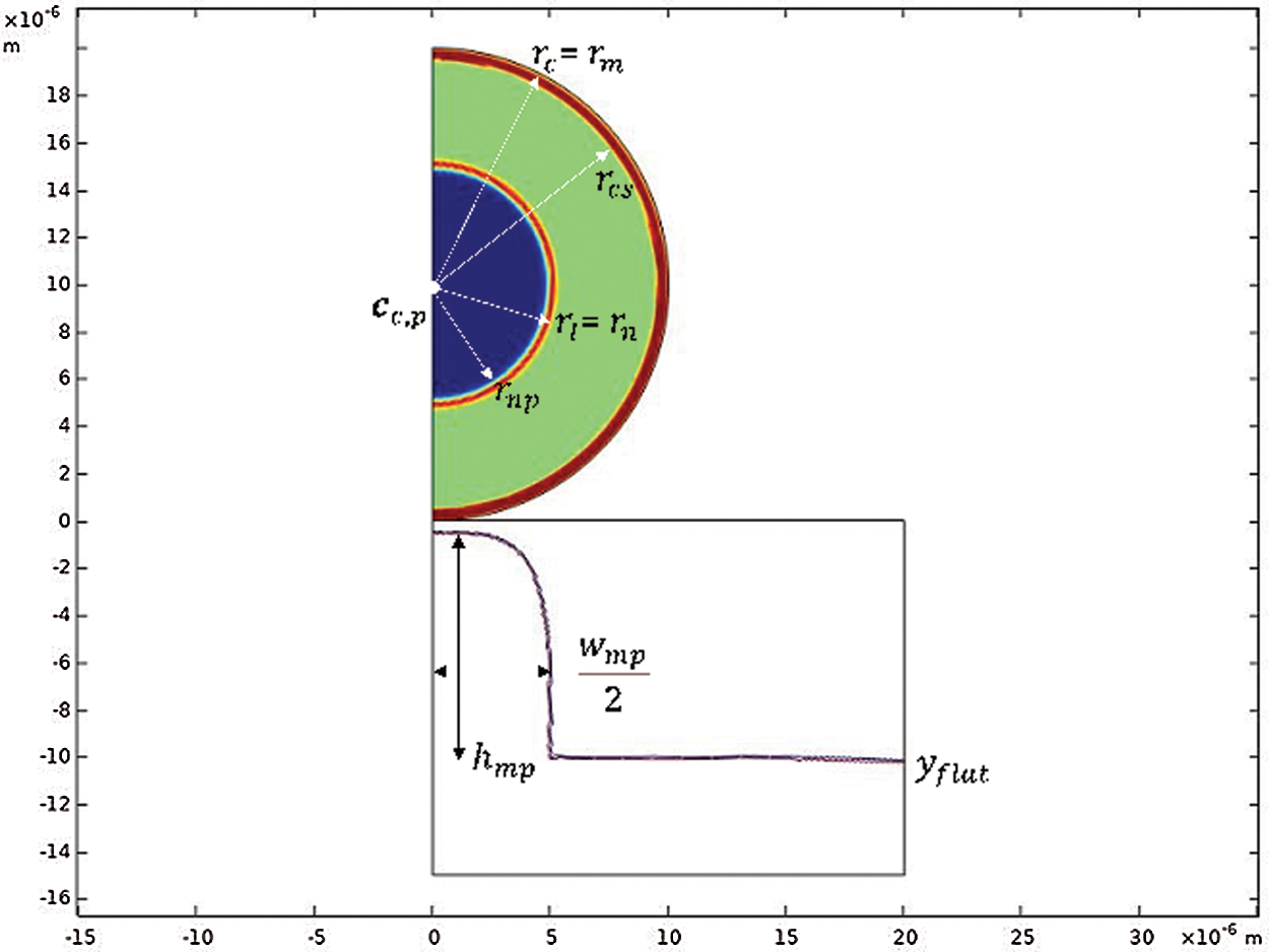
Figure 1: Cell and substrate geometry at t = 0 s. The cell has an external radius rc and it is constituted by the nucleus (nucleoplasm in blue and lamina in orange), external radius rn=rl , and the cytoplasm (cytosol in green and membrane in red), external radius rm . The substrate is constituted by a micropillar of height hmp and width wmp and a flat region placed at y-coordinate yflat

2.2 Constitutive Laws

Each cell component is composed of a solid and a fluid phase. To simplify the approach, we assume that both phases deform in parallel like in a Kelvin–Voigt model. Consequently, the overall stress S and the deformation F can be expressed as

S=csSs,i+cfSf (6)

F=Fs=Ff (7)

where the subscripts s and f indicate the solid and the fluid phases, respectively, while the subscript i indicates a specific constitutive law for the solid phase, as described in the followings (Section 2.2.1), and cs and cf the respective concentrations are given by

cs=cs,mgm+cs,csgcs+cs,lgl+cs,npgnp (8)

cf=cf,mgm+cf,csgcs+cf,lgl+cf,npgnp (9)

cs,m=1−cf,m (10)

cs,cs=1−cf,cs (11)

cs,l=1−cf,l (12)

cs,np=1−cf,np (13)

2.2.1 The Solid Phase

When describing the solid phase of an isotropic elastic material, for stability reasons, its strain energy must be poly-convex with respect to the three invariants I1 , I2 and I3 [27,28], which are expressed as follows:

I1=Tr(C) (14)

I2=det(C)Tr(C−1) (15)

I3=det(C) (16)

where C=FTF is the dilatation tensor.

From a physical point of view, I1 describes the length variations of the system in the three directions, I2 gives both the shear and length deformations and I3 describes the volume variations of the system [29,30]. Then, given the multistructural organization of the cell, it is important that all the invariants are considered. Nonetheless, in the present model, four different materials have been tested to point out their specific features. Specifically, we have implemented:

1.    A standard Saint-Venant material, which only depends on the first and second invariants I1 and I2 [31,32] and it is able to capture the deformations along the lines (i.e., the fibers deformations);

2.    A Neo-Hookean compressible material, which depends on the first I1 and third I3 invariants [33,34] and allows to take into account the deformations along the lines and inside the volumes (i.e., both fibers and cytosol plus nucleoplasm deformations);

3.    The Mooney-Rivlin and Yeoh compressible materials which depend on the three invariants [25,35] and describe the deformations along lines, volumes and surfaces (i.e., the membrane and the lamina). Furthermore, the Yeoh material takes into account the successive softening and stiffening behavior of an elastic material made of fibers.

The second Piola Kirchhoff stress Ss,i , where the subscript i indicates the material, is expressed as follows:

– for the standard Saint-Venant material Ss,SV reads

Ss,SV=λsTr(E)I+2μsE (17)

with λs=Eiυc(1+υc)(1−2υc)(1+υc) and μs=Ei2(1+υc) ( Ei and υc are the Young moduli of each cell component and the Poisson ratio, respectively), Tr the trace of a tensor, E the Green Lagrange tensor and I the identity matrix;

– for the compressible neo-Hookean material Ss,NH is given by

Ss,NH=μs(I−C−1)+λsln(J)C−1 (18)

with J=detF ;

– for the Mooney-Rivlin material Ss,MR can be written as

Ss,MR=2[αMR+βMR(TrC)]I−2βMRC+[λMRln(J)−2αMRJ2/3−4βMRJ4/3]C−1 (19)

with αMR=μs2−βMR , βMR=μs0.4 and λMR=λs+23μs [26];

– finally, for the Yeoh material Ss,Y reads

Ss,Y=2[αMR+βMR(TrC)+αY1(TrC)+αY2(TrC)2]I−2βMRC+[λMRln(J)−2αMRJ2/3−4βMRJ4/3]C−1 (20)

where αY1=−0.5αMR and αY2=0.1αMR are two constants [26].

2.2.2 The Fluid Phase

For the fluid phase of the cell, a Newtonian viscous fluid is considered but it must be defined in the Lagrangian configuration in order to ensure the compatibility with the solid phase. Thus, the Cauchy stress σf is classically given by

σf=λfTr(Df)I+2μfDf (21)

where λf and μf are the isotropic and deviatoric viscosities, respectively and Df must be expressed as a function of the rate of the dilatation tensor Cf as follows:

Df=Ff−TdCfdtFf−1 (22)

with the superscript T indicating the transpose of a matrix.

Since Cf=C and Ff=F (Eq. (7)), substituting σf in Eq. (21), we obtain the expression of the second Piola-Kirchhoff

Sf=Jλf2Tr(C−1dCdt)C−1−JμfdC−1dt (23)

2.3 The Gravity Force

The cell is submitted to the gravity force fg

fg=−ρctggiy (24)

where ρc is the initial cell density, g the gravitational acceleration and iy the vertical unit vector. tg is employed here to smoothly apply the gravity force to ensure the computation fast convergence. It is the composition of a regularized Heaviside function H and a level set function lg and it reads

tg=H∘lg=H∘(−t+Tg) (25)

with t the time and Tg a constant.

2.4 The Cell Environment

As the gravity is applied, the cell settles down and starts interacting with the underneath micropillared substrate, which is constituted by a micropillar and a flat region and it is defined by a characteristic function gs as follows:

gs=gmp+gflat=H∘(lmp+lflat)=H∘[−(x−xmpwmp)4−(y−ymphmp)4+1]+H∘[−y+yflat] (26)

where lmp and lflat are two level set functions, x and y are the actual coordinates of any point in the system, xmp and ymp define the position of the micropillars, wmp and hmp define the width and the height of the micropillar, respectively and yflat is the position of the flat region with respect to the y-axis.

Once the cell approaches the substrate, the contact force fct applies over a very thin layer corresponding to the intersection between the cell and the substrate. We have shown that fct can be approximated by a volume force [26] and it can be computed via a penalization technique as follows:

fct=μctgflatcof(F)nflat+μctgmpcof(F)nmp (27)

where μct is the penalization coefficient. cof(F) is the cofactor matrix defined as JcF−T and it is employed here to bring back to the initial configuration the outward normal vectors to the micropillar ( nmp ) and to the flat substrate ( nflat ), which are obtained as follows:

nmp=∇xlmp‖∇xlmp‖ (28)

nflat=∇xlflat‖∇xlflat‖ (29)

2.5 Finite Element Model

The global equilibrium of the system in the initial configuration can be expressed as

Divp(FS)+fg=ρca (30)

with Div the first order divergence operator in the initial configuration, and a the acceleration.

In order to employ a classical finite element approach, we multiply each term of Eq. (30) by the kinematically admissible displacement test function w and we integrate over the cellular domain Ωc . Then, by using some algebraic operations and by applying the Stokes theorem, we obtain

−∫ΩcTr[FS(Dpw)T]dVp+∫∂Ωc(w,FS(nc))dSp+∫Ωc(ρpg−ρpa,w)dVp=0 (31)

where nc is the outward normal to the cell and the first and the third term indicate the internal cellular stress and the volume forces, respectively. The second term describes the surface forces applied to the cell and specifically the contact force fct between the cell and underneath micropillared substrate. As mentioned above (Section 2.4), fct is applied through a very thin layer. Thus, the surface integral in Eq. (31) can be written as a volume integral over the penalization thickness hp . Therefore, Eq. (31) becomes

−∫ΩcTr[FS(Dpw)T]dVp+∫Ωc(ρcg+hpfct−ρca,w)dVp=0 (32)

Eq. (26) has been manually implemented using the weak form tool in COMSOL Multiphysics. The spatial discretization is obtained via quadratic polynomials for each isoparametric element of the mesh (mesh size between 0.3 µm and 1 µm). The time discretization is achieved via a second-order backward differentiation formula (BDF). The solution is computed using a nonlinear Newton scheme with a relative tolerance of 1% on the displacement error estimation.

3  Results and Discussion

The radii of the cell ( rc ) and the nucleus ( rn ) have been set equal to 10 µm and 5 µm, respectively. The membrane and the lamina have a thickness tm and tl of 0.5 µm and 0.1 µm [36], respectively (Fig. 1). The cell density ρc and the Poisson ratio υc have been set to 1000 kg/m3 and 0.45, respectively. The isotropic ( λf ) and deviatoric ( μf ) viscosities are equal to 1000 Pa·s and 5 × 10−3 Pa·s, respectively. The Young’s moduli have been set to Em = 100 Pa [31], Ecs = 10 Pa [37], El = 1000 Pa [31,38] and Enp = 10 Pa [39]. The gravity force is gently applied on the cell and reaches its maximum at 2 Tg=10000s . Through the gravity, the cell comes in contact with the micropillar which has a width ( wmp ) and a height ( hmp ) of 20 µm and 9.5 µm, respectively (Fig. 1). All the simulations last for Tend = 18000 s. All the parameters of the model are listed in Table 1. For each series of simulations that we are going to present, the nucleus stress has been evaluated in terms of Mises Cauchy stress σMises , whereas the strains have been quantified through three variables: (i) J1 = I1 = Tr(C) to detect the fibers elongation, (ii) J2 = Tr(C2) to evaluate the shear and length deformations and (iii) J3 = I3 = det(C) to assess the surface variations.

3.1 Cell Components Constitutive Law

For the first series of simulations, we have tested different constitutive laws for the cell components. All the parameters defining each constitutive law are reported in Table 1. The fluid coefficients have been set equal to cf,m=cf,cs=cf,l=cf,np=0.5 .

The Saint-Venant material model is the simplest and mostly used in the literature, but it is not robust enough to describe very large deformations. The Neo-Hookean and the Mooney-Rivlin materials are efficient in considering large strains, but they do not exhibit typical stiffness-softening followed by hardening during deformation. Finally, the Yeoh model is theoretically the most consistent, but it is much more complex than the others due to a higher number of parameters to define (Eq. (21)).

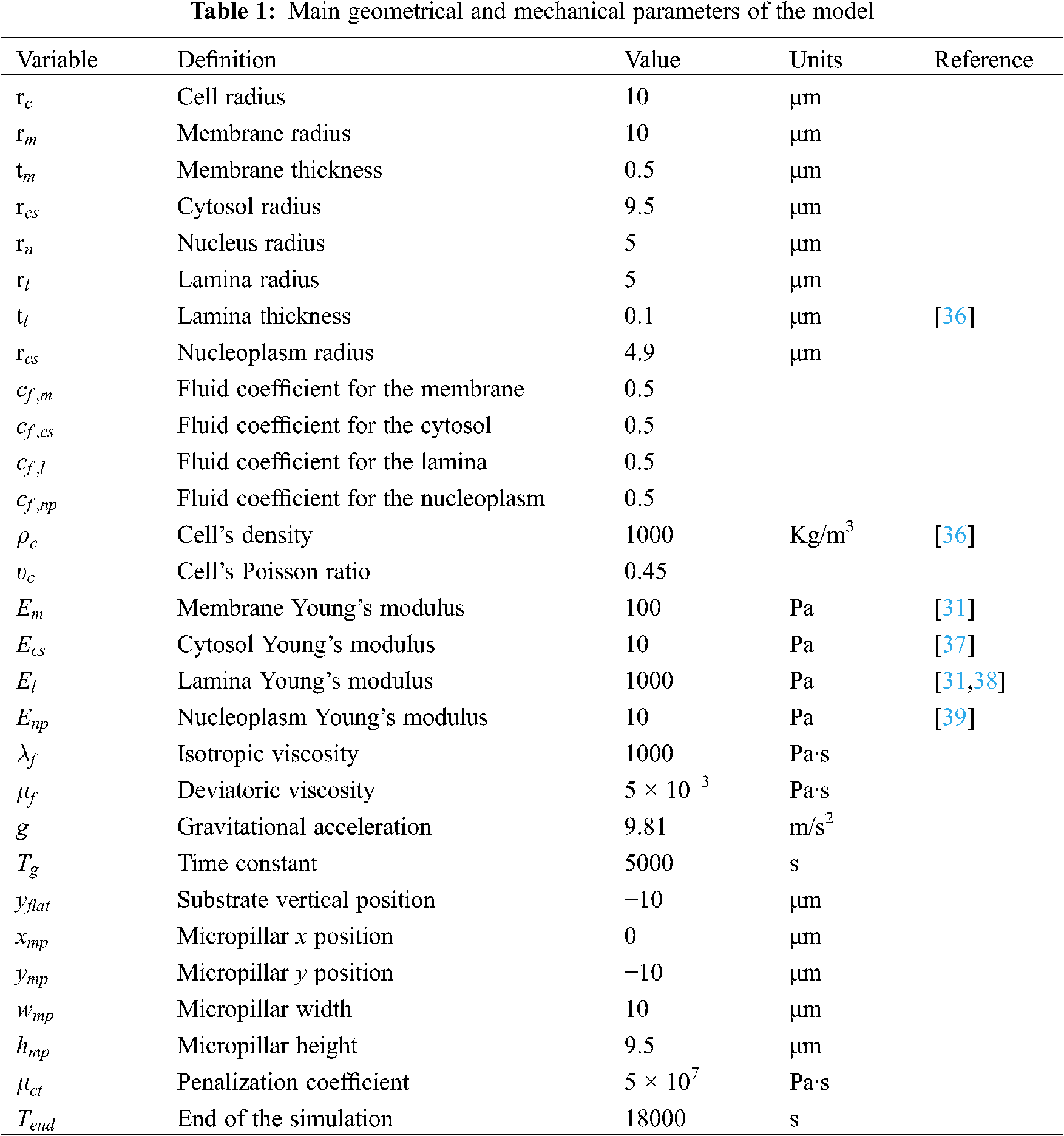
The evolution as a function of time of the Mises stress σMises and J1 , J2 and J3 in the nucleus Ωn are shown in Fig. 2. The highest value of the von Mises stress (1.042 Pa) is obtained for the Mooney-Rivlin material (Fig. 2a). The Neo-Hookean and the Yeoh materials are very close with a maximum of 1.032 Pa and 1.027 Pa, respectively. For the Saint-Venant material, the maximum is slightly lower (0.86 Pa).

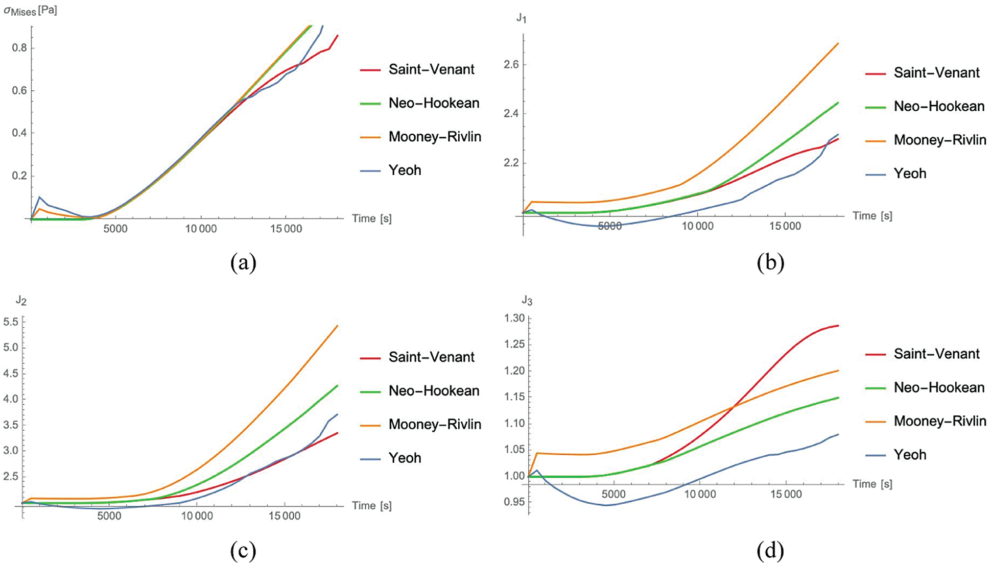
Figure 2: von Mises Cauchy stress σMises (a) and J1 (b), J2 (c) and J3 (d) in the nucleus Ωn as a function of time for different materials: Saint-Venant (red line), Neo-Hookean (green line), Mooney-Rivlin (orange line) and Yeoh (blue line)

For the strains, the Mooney Rivlin material provides the maximum values of J1 and J2 (2.68 and 5.44, respectively) and J3=1.20 (orange line in Figs. 2b, 2c and 2d). For the Saint-Venant material, J1 = 2.30, J2 = 3.35 and J3 = 1.28 (red line in Figs. 2b, 2c and 2d). The Yeoh material shows low values for all the three strains indicators, more specifically J1 = 2.31, J2 = 3.72 and J3 = 1.08 (blue line in Figs. 2b, 2c and 2d). The Neo-Hookean material provide J1 = 2.44, J2 = 4.27 and J3 = 1.15 (green line in Figs. 2b, 2c and 2d).

We can estimate the contribution of the nucleus to the total cell deformation. In terms of fibers elongation ( J1 ), we found that when implementing the Mooney Rivlin material the nucleus undergoes 56% of the global deformation, whereas with the Saint-Venant material only 49%. Regarding the shear and length variations ( J2 ), the Mooney Rivlin ensures again the highest nucleus contribution (81%) vs. the Yeoh material for which the nucleus supplies for only 61%. Finally, for the surface variations ( J3 ), contributions between 18% (Saint-Venant material) and 23% (Mooney Rivlin material) are found. In Fig. 3 we show the overall deformation of the cell and the nucleus at t = 18000 s for the different material models.

Figure 3: Total cell deformation at t = 18000 s for the Saint-Venant (a), the Neo-Hookean (b), the Mooney-Rivlin (c) and the Yeoh (d) material (blue = nucleoplasm, orange = lamina, green = cytosol, red = membrane)

Since the cell is composed by several organelles having different structures and geometries, there is a need for a constitutive macroscopic law able to describe the stresses associated to such heterogeneous strains. More specifically, taking into account these stresses implies low values of J1 , J2 and J3 . Thus, according to our results, the Yeoh material model seems to be the most appropriate, which confirms the theoretical remarks at the beginning of the section.

3.2 Nucleus Fluid and Solid Phases

For the second series of simulations we have evaluated the influence of the fluid-solid phases of the lamina and of the nucleoplasm on the nucleus behaviour. Specifically, we have let vary cf,l and cf,np from 0.1 to 0.9, testing all the combinations for a total of 24 simulations (one combination has not converged, i.e., cf,l=cf,np=0.9 ). The values of cf,m and cf,cs have been set to 0.5. The Young moduli of the cell organelles are those defined at the beginning of Section 3.

In Fig. 4, values of σMises (Fig. 4a) and of J1,J2 and J3 (Figs. 4b, 4cand 4d) in the nucleus Ωn are presented. σMises is maximal for cf,l=0.1 and cf,np=0.7 and it is equal to 1.32 Pa.

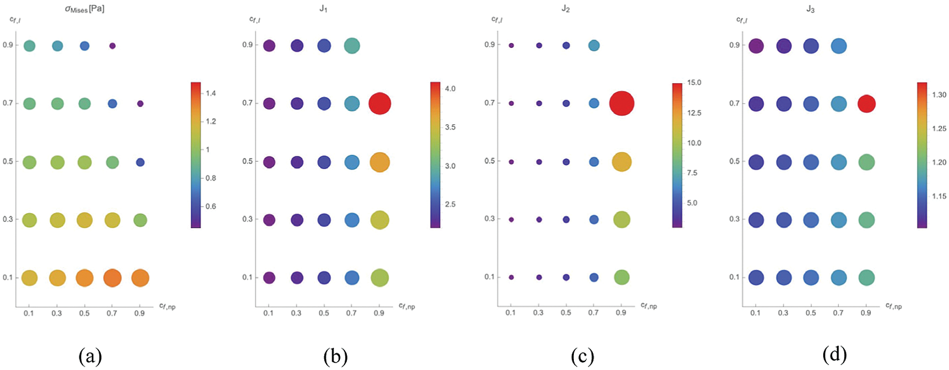
Figure 4: Maximal value of σMises (a) and J1 (b), J2 (c) and J3 (d) in the nucleus Ωn at t = 18000 s as a function of El and Enp

On the one side, the maximal strains are found for cf,l=0.7 and cf,np=0.9 and they are equal to J1=4.08 (71% of the total cell deformation), J2=15.20 (163% of the total cell deformation) and J3=1.31 (20% of the total cell deformation). This combination corresponds to σMises=0.45 Pa. In Fig. 5a, the total deformation of the cell organelles at t = 18000 s is shown and one can notice that the nucleus is particularly stretched. Such a large strain could exacerbate the sensor functions of the nucleus as it has been observed in previous experimental studies [40–42] and therefore induce cell motility via the activation of specific stretch-sensitive proteins.

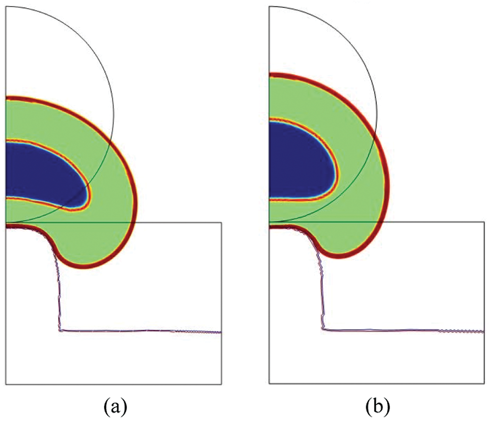
Figure 5: Total cell deformation at t = 18000 s for cf,np=0.9 and cf,l=0.7 (a) and for El=1000 Pa and Enp=10 Pa (b) (blue = nucleoplasm, orange = lamina, green = cytosol, red = membrane)

On the other side, the lowest values of J1 and J2 ( 4.08 and 15.20 , respectively) are found for cf,l=0.3 and cf,np=0.1 , with σMises=1.08 Pa, and they correspond to 51% and 58% of the total cell deformation. Whereas the minimal value of J3 (1.31) has been obtained for cf,l=0.9 and cf,np=0.1 , with σMises=0.85 Pa, and it corresponds to 23% of the total cell deformation.

3.3 Nucleus Mechanical Properties

For the last series of simulations, we have let vary the Young’s moduli of the nucleoplasm ( Enp ) and of the lamina ( El ). Specifically, we have set Enp = 10, 30, 50, 70, 90 Pa and El = 1000, 1500, 2000, 2500, 3000 Pa for a total of 25 simulations, which have all converged. For the fluid and solid phases of the organelles, we have set here cf,np=cf,l=cf,cs=cf,m=0.5 .

Fig. 6, we show the results in terms of Mises Cauchy stress σMises (Fig. 6a) and of J1,J2 and J3 (Figs. 6b, 6c and 6d) in the nucleus Ωn . σMises is maximal for Enp = 10 Pa and El = 2000 Pa and it is equal to 1.47 Pa. The maximal values of J1 and J2 are observed for Enp = 10 Pa and El = 1000 Pa ( σMises=1.03 Pa) and they are equal to 2.44 (53% of the total cell deformation) and 4.27 (69% of the total cell deformation), respectively) (Fig. 5b). For J3 , the maximal value is equal to 1.16 (22% of the total cell deformation) and it is found for Enp = 10 Pa and El = 3000 Pa, with σMises=1.47 Pa. As for the minimal values of J1 and J2 , they are equal to 2.11 (50% of the total cell deformation) and 2.26 (51% of the total cell deformation), respectively. They are found for Enp = 90 Pa and El = 1500 Pa and provide σMises=0.55 Pa. The lowest J3 has been found equal to 1.10 (24% of the total cell deformation) for Enp = 90 Pa and El = 1000 Pa with σMises=0.46 Pa.

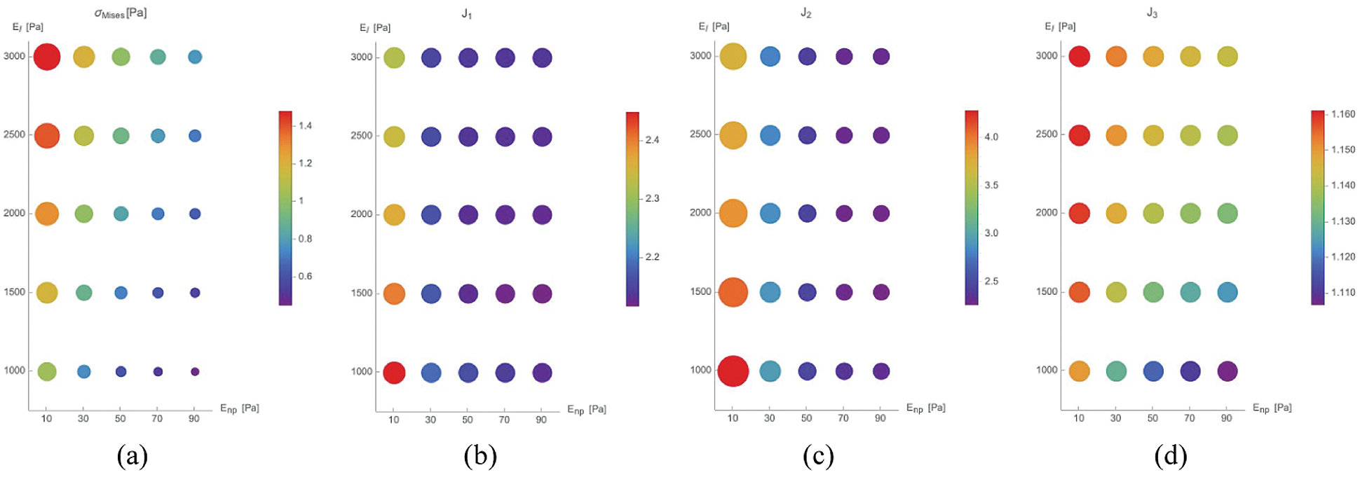
Figure 6: Maximal value of σMises (a) and J1 (b), J2 (c) and J3 (d) in the nucleus Ωn at t = 18000 s as a function of cf,np and cf,l

3.4 Comparison with Experimental Data

In the previous series of simulations, tend has been set equal to 18000 s. In this section we propose to go further ( tend = 24000 s) in order to explore more severe nucleus deformations and to be able to compare our numerical results with experimental observations.

We have run three additional simulations ( S1 , S2 , S3 ) for which a Saint-Venant material model has been implemented. However, the mechanical properties of the nucleus (i.e., Enp and El ) as well as the nucleus fluid concentration (i.e., cf,np and cf,l ) have been modified as reported in Table 2.

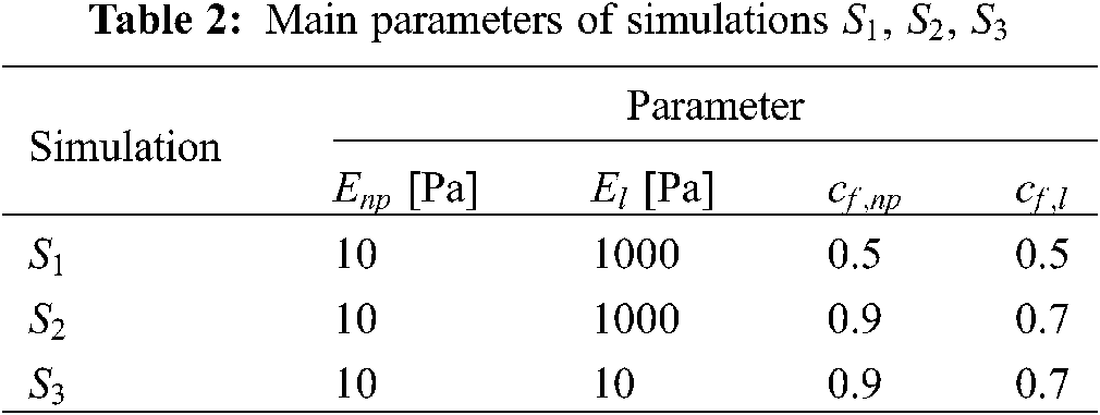
From a quantitative point of view, the results in terms of maximal stress ( σMises ) and strain ( J1 , J2 , J3 ) in the nucleus Ωn are reported in Table 3.

In Fig. 7, the total cell and nucleus deformation at t = 24000 s is shown. One can notice that for S1 (Fig. 7a), the final shape of the nucleus is not significantly different from the previous simulations. However, as the fluid concentration of the nucleoplasm and the lamina is increased ( S2 ), the nucleus undergoes a higher deformation (Fig. 7b) leading to an important reduction of the distance between the nuclear lamina and the micropillar boundary. Additionally, the nucleus starts acquiring a ‘peanut’ shape as it has been experimentally observed for different cellular phenotypes including mesenchymal stem cells, osteosarcoma cells and bone marrow stroma cells [11–14]. Such an outcome becomes even more evident when the nuclear lamina is ablated ( S3 ) (Fig. 7c), which correspond to a decrease of the lamina Young’s modulus in the numerical simulation. This confirms specific experimental observations according to which tumor cells are able to soften their nucleus and adjust their mechanical properties in order to facilitate extravasation [43].

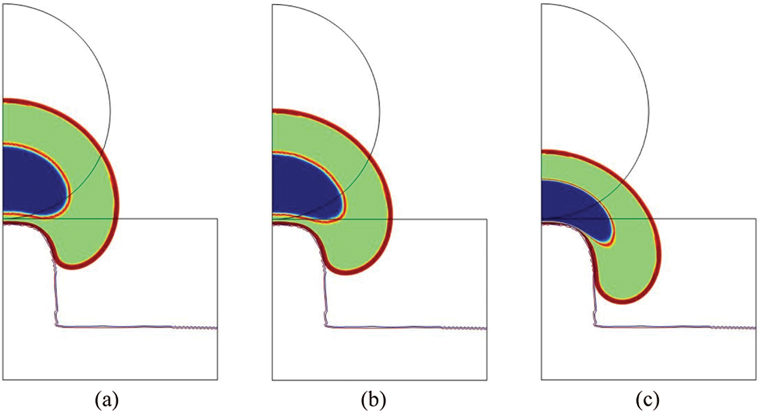
Figure 7: Total cell deformation at t = 24000 s for S1 (a), S2 (b) and S3 (c) (blue = nucleoplasm, orange = lamina, green = cytosol, red = membrane)

In [12–14] a shape index (SI) parameter is used to quantify the nucleus self-deformation. SI is defined as follows:

SI=4πSl2 (33)

where S and l are the nucleus surface and perimeter, respectively. SI is equal to 1 for a perfect circle (i.e., no deformation), whereas it is equal to 0 for a straight line. In [12–14], SI is measured in the plan perpendicular to the micropillars. This is not possible in our model since we are in 2D. Nonetheless, we believe that it is even more interesting to measure SI in the sagittal plan to quantify the nucleus self-deformation, but also its penetration. We found that SI is equal to 0.32, 0.26 and 0.21 for S1 , S2 and S3 , respectively indicating a significant nucleus deformation in particular when the nuclear lamina is ablated (i.e., S3 ).

4  Conclusions

In this paper we have presented a 2D computational model to investigate the interactions between the cell and the micropillared substrate. The cell is initially suspended and gently meets the pillar due to the gravity force. Then, the contact force between the cell and the pillar is applied over a very thin layer.

The model is equipped with specific mechanical tools, namely the constitutive laws describing the cell components, their mechanical properties, and the fluid and solid phase mixture for each component. Our main objective has been establishing a correlation between such elements and the nucleus stress-strain state. To do so, a thorough sensibility study has been performed. More specifically, three series of simulations have been run: (i) the first one involves different materials models to describe the cell behaviour, i.e., Saint-Venant, Neo-Hookean, Mooney-Rivlin and Yeoh materials, (ii) the second one focuses on the balance between the fluid and solid phases of the lamina and nucleoplasm, (iii) the third one takes into account the variation of the mechanical parameters (i.e., the Young modulus) of the lamina and the nucleoplasm.

Through the large spectrum of combinations that we have provided, biologists may identify the one corresponding to specific cellular phenotypes or behaviors. Additionally, our model could inspire further experimental investigations to explore the interactions between the cell and the micropillared substrate.

We have been able to quantify the stress and the strain in the nucleus Ωn . For the former, the Mises Cauchy stress σMises has been assessed. For the latter, we have computed J1 , J2 and J3 which provide the fibers elongation, the shear and length variations and the surface variations, respectively.

We have shown that the variation of the balance between the fluid and solid phase of the nucleus induces the maximum strains of the nucleus. In fact, we have found that varying cf,l and cf,np provides the highest values of J1,J2 and J3 . More specifically, J1 and J2 are equal to 4.08 and 15.20 for cf,l=0.7 and cf,np=0.9 and such values are much higher than those found for different constitutive laws (2.68 and 5.244 for the Mooney Rivlin material) and for different values of Enp and El (2.44 and 4.27 for Enp = 10 Pa and El = 1000 Pa). For J3 , the maximal values are closer although the highest value (1.31) is still found for the sensibility study on the fluid and solid phases balancing. This outcome confirms the importance of the phases balance and the need to correctly take them into account in the mechanical description of the nucleus. Furthermore, the amount of strain found could have an impact on the nucleus response and more particularly on the expression of strecth-sensitive proteins which could be responsible of cell motility in confined environments [40–42].

In terms of stress, even though the maximal values of the Mises Cauchy stress σMises are very close for the three series of simulations, the highest one (1.47 Pa) is found when varying the Young moduli of the lamina and the nucleoplasm. More specifically, such a value is obtained when Enp = 10 Pa and El = 2000 Pa. This configuration could potentially induce the lamina rupture due to its high stiffness compared to the nucleoplasm. Such a phenomenon can change the lamina structure and therefore have critical consequences in disease like cancer or in genome stability [44–46].

Through some additional simulations, we have been able to compare our numerical results to the experimental observations on different cellular phenotypes. More specifically, we have shown that by increasing the simulation time, the nucleus undergoes significant self deformation and it acquires a ‘peanut’ shape by embracing the micropillar as it has been reported in [11–14]. Such a phenomenon is exacerbated when the nuclear lamina is ablated (i.e., reducing the Young modulus) and it confirms data according to which tumor cells are able to adjust their mechanical properties in order to invade healthy tissues [43].

To conclude, our model, which has been built only using mechanical tools, has drawn a large spectrum of scenarios to analyze and quantify the nucleus stress-strain state. It can help identifying the mechanical features responsible for specific nucleus responses and their impact on the global cell behavior. Although the interesting results, the present model could be improved in the different ways. First, a three-dimensional description of the system would allow to better evaluate the interactions between the cell and its surroundings and the nucleus role. Secondly, it could be interesting to quantify the pressure gradient in the cell in order to assess the proteins traffic flow to and from the nucleus. Finally, a precise description of the structure of the nuclear lamina could provide new information regarding its rupture and remodelling.

Funding Statement: The authors received no specific funding for this study.

Conflicts of Interest: The authors declare that they have no conflicts of interest to report regarding the present study.

This work is licensed under a Creative Commons Attribution 4.0 International License, which permits unrestricted use, distribution, and reproduction in any medium, provided the original work is properly cited.