| Structural Durability & Health Monitoring |
DOI: 10.32604/sdhm.2021.016975
ARTICLE
A TimeImageNet Sequence Learning for Remaining Useful Life Estimation of Turbofan Engine in Aircraft Systems
Department of Computer Science & Systems Engineering, Andhra University College of Engineering (A), Visakhapatnam, India
*Corresponding Author: S. Kalyani. Email: kalyaniakiri3009@gmail.com
Received: 15 April 2021; Accepted: 14 September 2021
Abstract: Internet of Things systems generate a large amount of sensor data that needs to be analyzed for extracting useful insights on the health status of the machine under consideration. Sensor data of all possible states of a system are used for building machine learning models. These models are further used to predict the possible downtime for proactive action on the system condition. Aircraft engine data from run to failure is used in the current study. The run to failure data includes states like new installation, stable operation, first reported issue, erroneous operation, and final failure. In the present work, the non-linear multivariate sensor data is used to understand the health status and anomalous behavior. The methodology is based on different sampling sizes to obtain optimum results with great accuracy. The time series of each sensor is converted to a 2D image with a specific time window. Converted Images would represent the health of a system in higher-dimensional space. The created images were fed to Convolutional Neural Network, which includes both time variation and space variation of each sensed parameter. Using these created images, a model for estimating the remaining life of the aircraft is developed. Further, the proposed net is also used for predicting the number of engines that would fail in the given time window. The current methodology is useful in avoiding the health index generation for predicting the remaining useful life of the industrial components. Better accuracy in the classification of components is achieved using the TimeImagenet-based approach.
Keywords: Multivariate sensor data; TimeImageNet; Remaining life estimation; machine learning; 2D image; Convolutional Neural Network
Abbreviations
| PHM | Prognostics and Health Management |
| RUL | Remaining Useful Life |
| C-MAPSS | Commercial Modular Aero-Propulsion System Simulation |
| DL | Deep Learning |
| DNN | Deep Neural Network |
| CNN | Convolutional Neural Network |
| AE | Auto-Encoders |
| DBN | Deep Belief Networks |
| RNN | Recurrent Neural Networks |
| LSTM | Long-Short Term Memory |
| PCA | Principal Component Analysis |
| LDA | Linear Discriminant Analysis |
| LLE | Locally Linear Embedding |
| KPCA | Kernel PCA |
| MLP | Multilayer Perceptron |
| SVM | Support Vector Machine |
| FFNN | Feed-Forward Neural Network |
| LPC | Low-Pressure Compressor |
| HPC | High-Pressure Compressor |
| HPT | High-Pressure Turbine |
| LPT | Low-Pressure Turbine |
| ReLU | Rectified Linear Unit |
| tanh | hyperbolic tangent |
| RMSE | Root Mean Square Error |
| MSE | Mean Square Error |
| RMSprop | Root Mean Square propagation |
Data Generated from Internet of Things (IoT) systems is increasing enormously due to the availability of various sensors and low-cost Internet. Machine condition monitoring based on sensor data is crucial in generating insights from sensor data in multiple domains. The objective of IoT systems is primarily to monitor the failure mechanisms to illustrate the way that complex machines run for ages and fail. To extract the health status of a machine under consideration, a systematic relation is to be established between the failure mechanisms and the life-cycle management of a system. The aim of finding out the health status of a machine is to maximize its operational availability by adopting functions of condition monitoring, state assessment, prognostics, failure progression, and diagnostics. Such a study can lead to avoiding the sudden breakdown of machines during operation. Hence, there is a need to develop methods to evaluate the sequence of events and their consequences on the device pertaining to its status.
Time series of sensors are to be analyzed to find the patterns in the data, which are useful to generate alarms or trigger indications to avoid catastrophic failure. As the data is generated from sensors of various research fields and the plethora of digital machines, high-performance sequence methods are needed to apply on them. Most of the data points collected from significant sources of IoT applications are not independent and identically distributed. They result from time-series measurements at successive time intervals. Finding the relation between independent variables and outcome variable has to be done using multiple models. A new model of analyzing sequential data to enable pattern recognition is required. At the initial level of a complex system’s lifetime, maintenance of the system is not necessary as the components of the system will be in proper working condition. During the initial stage of usage, the system’s health status will be generally stable, and every operational trajectory will have its fixed health level. This stable health status continues to persist until a critical time and eventually reduces when an early incipient fault condition manifests. With continued operation and progress in time, the probability of system failure increases, eventually resulting in system degradation leading to a catastrophic failure. If the equipment’s life can be measured with accuracy ahead of time, necessary maintenance and management measures can be taken to ensure proper reliability and effectiveness of the equipment. Early identification of failure and damage is often critical in determining the Remaining Useful Life (RUL) of the equipment. Consequently, it is crucial to forecast equipment life.
The turbofan engine is a complex and critical part of a sophisticated aircraft system, and a simplified diagram of the engine is shown in Fig. 1. Unexpected breakdown in the engine may lead to a severe loss of human lives and increased cost of repair. Hence reliable maintenance of an aircraft engine poses a challenge with respect to its decrease in downtime and cost of maintenance to ensure the availability of a healthy engine. To prevent unplanned downtime and reduce the cost of maintenance, an optimal maintenance strategy that detects the degradation pattern is required before the engine fails. Various maintenance strategies have been evolved over time from traditional methods as reported by Gouriveau et al. [1] for the predictive maintenance of turbofan engines. Ding et al. [2] proposed that the traditional methods are either reactive or proactive where the engine component is replaced after unexpected breakdown, or the maintenance tasks are scheduled assuming the level of degradation initiated and progressed over time. In the current scenario, both methods are inadequate to eradicate faults. Therefore, an intelligent predictive maintenance strategy is needed as proposed by Kalyani et al. [3] to coordinate the scheduling tasks of maintenance based on failure diagnosis, RUL estimation, and fault prognosis.

Figure 1: Simplified diagram of an engine simulated in C-MAPSS (Commercial Modular Aero-Propulsion System Simulation). N1: Turbine axis, LPC: Low Pressure Compressor, N2: Turbine shaft, HPC: High Pressure Compressor, LPT: Low Pressure Turbine, HPT: High Pressure Turbine
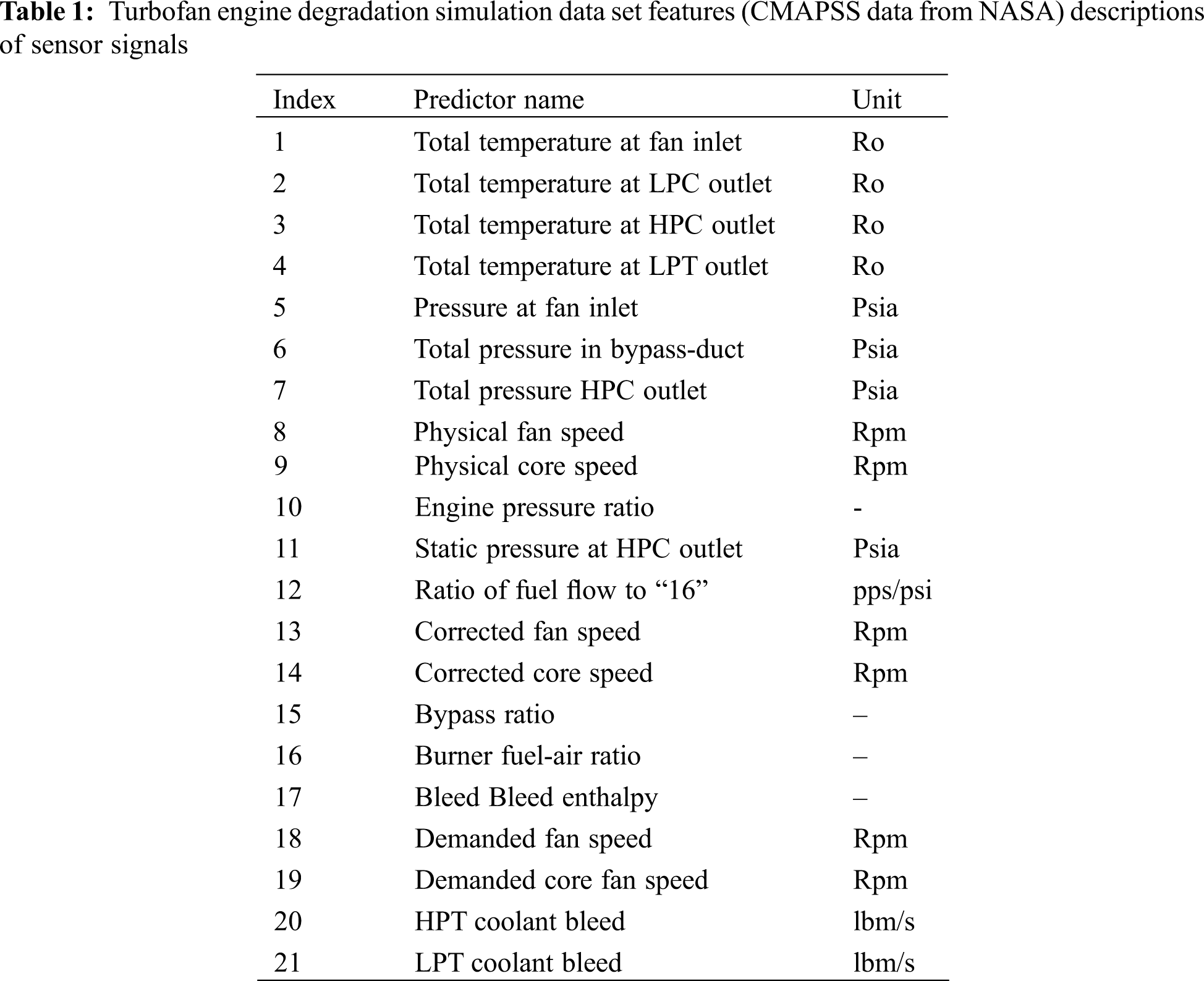
Different types of measurement carried out are: (i) Temperature measurement, (ii) Pressure measurement, (iii) RPM measurement (iv) Air Mass flow measurement and the dataset features are given in Table 1.
Prognostics and Health Management (PHM) in predictive maintenance offers various advantages to prevent catastrophic failures. Atamuradov et al. [4] illustrated that the major contributions of PHM are fault detection, isolation of faults, and prognosis of failures that allow estimation of RUL and make suitable decisions for maintenance. The major role of PHM is to estimate RUL with high accuracy to overcome unexpected failures. Gouriveau et al. [5] classified the several RUL methods into three categories (i) physics-based approach, (ii) data-driven approach, and (iii) hybrid approach. Physics-based approach needs extensive knowledge of the physical background and is based on the mathematical model of algebraic or differential equations. These models are primarily suitable to predict RUL when the available data is limited and insufficient. The data-driven approach, however, predicts RUL when sufficient failure data is available. Data-driven models are highly promoted and used by researchers with advanced technologies that are adopted in the industrial systems for collecting and monitoring the data. Hybrid approaches are the ones that estimate RUL combining both the physics-based and data-driven based approaches.
Increase in the high dimensionality of data collected from multiple sensors of a complex system leads to a critical challenge of extracting the relevant features of performance degradation, thereby affecting the efficiency of prediction reported by Sharma et al. [6]. The manual feature extraction methods for such complex systems require substantial human labor, where in most of the information is either lost or uncertain in its performance. Yang et al. [7] proposed traditional and familiar unsupervised feature extraction methods like Principal Component Analysis (PCA) and Linear Discriminant Analysis (LDA). They project the high dimensionality of data to a low dimensional space using data correlation but suffer from the linear projection. Tenenbaum et al. [8] and Roweis et al. LLE [9] proposed nonlinear feature extraction methods ISOMAP and LLE. These methods follow a predetermined way of extracting, which may not be suitable for low-dimensional space. Besides the above, machine learning and deep learning-based methods are introduced by LeCun et al. [10] to treat the highly varying and nonlinear raw data to overcome the human labor in designing features.
Traditional multivariate time series analysis like Simple Exponential Smoothing (SES) and Autoregressive Integrated Moving Average (ARIMA) were used to analyze high-dimensional data. But in due course, several machine learning models such as Linear Regression, Logistic regression, Decision Trees, Support Vector Machines are also proposed to solve the prediction and classification problems. Advancement of deep learning technology and graphical processing motivated the researchers to use deep learning techniques to estimate the RUL with better accuracy. Deep learning-based hierarchical structures include various stacked processing layers that automatically learn high-level representations from the high dimensional space, and thereby improve the classification or prediction. In general, deep learning algorithms outperform the conventional machine learning algorithms, that include ANN, DNN, LSTM, DBN, and CNN. The various deep learning algorithms are reviewed and classified into discriminative and generative models. Discriminative models are constructed based on feature engineering and model tuning that automatically learn the mapping between multivariate data inputs and the classification results, where generative models are model-based classifiers that perform an unsupervised initial training step followed by the learning phase of the classifier. The most prevalent and widely used RUL prediction architectures are adapted to a single method like CNN, DNN or RNN applied directly to raw multivariate data.
The present work is aimed at an innovative image-based feature engineering technique for preprocessing as a discriminate deep learning model. The raw form of multivariate data is first encoded into images considering various batch sizes of sequence lengths. The concept of feature extraction, involves transforming the raw input data into images to achieve more accurate predictions.
The major contributions of the present work are as the following:
• To extend the 2D image transformation method for Multivariate Time Series classification from the univariate time series input to Multivariate inputs.
• The innovative image concatenation method transforms one batch of data into multiple images, combines them as single two-dimensional image aggregation, and provides multiple channels for Convolution Neural Network.
• The same process is experimented with various sequence lengths for different batches of data to investigate classification and prediction accuracy by using the relatively simple network.
• The results show that selecting the size of the sequence length in the image transformation method contributes significantly to improve the classification and prediction accuracy.
The present paper is structured as follows: Section 2 provides a review of deeplearning models applied on the NASA C-MAPSS dataset, data encoding method, and convolution neural network architecture. Section 3 describes the methods adapted for data transformation, image aggregation variants, and the hyperparameter setting. The Implementation is discussed with a specific turbofan engine dataset in Section 4. The experimental results and effectiveness of the proposed model are illustrated in Section 5 followed by conclusions in Section 6.
Multivariate time series (MTS) data accessible from various sources may be used to determine the operating status or health of the devices. Yang et al. [11] developed a binary classification model using a machine-learning algorithm to classify defects from collected time-series data to improve production quality in smart manufacturing. Wang et al. [12] categorize the current Time-Series Classification approaches from various perspectives. Spectral analysis and wavelet analysis are examples of frequency-domain methods, while auto-correlation, auto-regression, and cross-correlation analysis are examples of time-domain methods. In terms of classification strategy, there are two types: instance-based and feature-based approaches. The former uses the Euclidean distance-based 1-Nearest Neighbor (1-NN) proposed by Xing et al. [13] to quantify the similarity between any incoming test sample and the training set and assigns a mark to the most similar class. Joeng and coauthors [14] Dynamic’s Time Wrapping (DTW) is also a common and widely used method in this category. Optimal classification boundaries were sought by Eads and coinvestigators [15], Nanopoulos and coworkers [16], and Rodigrez et al. [17] in order to derive more discriminative and representative features for use by a pattern classifier. Eckmann and coworkers [18] given the method of recurrence plots to visualize the repeated patterns of dynamic systems. Silva and coinvestigators [19] used this tool to compare recurrence plots of time series and suggested the use of a compression distance approach to calculate similarity. Methods focused on mapping from time series to network based on the network’s topology, which is used as a way to characterize the time series suggested by Donner et al. [20] and Campanharo et al. [21]. Since many of these approaches do not allow a reconstruction of the original data, it’s difficult to tell how topological properties apply to time series. Wang et al. [22] suggested three techniques to image time series, two based on Gramian Angular Fields (GAF) and one based on Markov Transition Fields (MTF). The majority of time series problems, such as classification (e.g., Fulcher et al. [23] and Lei et al. [24]); time-series clustering (e.g., Aghabozorgi et al. [25]; Bandara et al. [26]); and anomaly detection (e.g., Hyndman et al. [27]), are due to feature representations. Nonetheless, the network structure and hyper-parameters setting has a significant impact on the performance of neural networks. When it comes to achieving higher output in a mission, a deeper layer is often needed. Therefore, a lot of computing power is needed. Our time series imaging approach has the advantage of having many well-trained neural network models for imaging classification. Based on the pre-trained model with ImageNet, we fix the parameters of the previous layers and fine-tune the last few layers for our mission. Malhotra et al. [28] built TimeNet, a deep recurrent neural network for extracting features from time series. Fawaz et al. [29] published a recent survey on promising deep neural network applications for time series classification in a variety of fields. It transforms signals using down sampling and smoothing operators, followed by a local convolution point, to extract features at different frequencies and scales. On multichannel time-series signals of human activities, a deep CNN is used. Zheng et al. [30] proposed supervised feature learning with ConvNet to identify time series data by explicitly using time series data as inputs. ConvNet was also used by Gamboa [31] for time series analysis, with positive results. Yazdanbakhsh and Dick transformed an image using same-size segments in a time series with a sliding window and a Dilated Convolution Neural Network for classification. Rather than using raw time series data as input, Wang et al. [32,33] transformed univariate time series data into various images, such as Gramian Angular Fields (GAF) and Markov Transition Fields (MTF), which were then used as ConvNet inputs. In fact, this image-based paradigm gave birth to a new branch of deep learning approaches that involve image transformation as a feature engineering technique. The computer vision feature extraction principle was used to inspire the transformation of time series into photographs. The spatially invariant filters (or features) are learned from raw input time series, where the ConvNet approach alleviated the problems of (1) temporal information loss and (2) the learned features no longer being time-invariant, which are both problems with conventional multi-layer-filtering methods. Chen et al. [34] used the same structure, RPMCNN (Relative Position Matrix with ConvNet), to perform classification using transform 2D images from time-series data as inputs in their most recent work. Encoding univariate time series data to 2D images as an input to ConvNet yielded promising results for all of them. The operating status or the health condition of the machines can be identified from the joint learning of feature representation, and the selection of sequence length for recurrence plot fed into CNN increases the regression and classification performance.
Major advantage of using recurrence plots is to encode multivariate time series data to graphically used images. The visual representations inspect the higher dimensional phase space trajectories. In addition, the resultant image obtained provides insights into the way time series data evolved over time. Four different topologies based on the characteristics the image exhibits, for time series data are given below.
• Homogeneous: typical of stationary and autonomous systems. For example, randomly generated time series.
• Periodic: the recurrence plot identifies oscillations even in systems where it is hard to recognize.
• Drift: typical of systems variables with slow variations over time.
• Disperse: abrupt changes are presented due to extreme events in the data.
Recurrence plots mainly focus on detecting hidden anomalies or rare events along with the series. A Recurrence plot identifies periodicity of the signal from the same repeated pattern observed over the two-dimensional space. The diagonal oriented lines presented by the oscillating systems show a mosaic architecture indicating that the states’ evolution is very common at various time points. In addition, anomalies are shown as isolated standalone points, and the duration of that constant state of being or a gradual state change is marked as the time length in the form of vertical or horizontal. Above all, the huge potential of dispersing structure in recurrence plots is to detect hidden anomalies. The transformed images reveal the hidden anomalies at a glance using recurrence plots. This benefits the process of detecting a rare event from the historical data by creating 2D images within a fixed time period to feed CNN. This procedure is similar to recognizing shapes from a picture or identifying a human face using CNN.
Convolution Neural Network (CNN) is widely used in recent times to detect meaningful insights and patterns in computer vision. A typical CNN architecture consists of a convolution layer, pooling layer, fully connected layer along with the input and output layers. The convolution layer uses a linear function to extract meaningful features like edge, color, and gradient orientation from the input image. The resultant matrix is a dot product with a filter covering the input image. The popular activation function, such as ReLU, plays a nonlinear role between the convolution and pooling layers to reduce the vanishing gradient problem to improve the performance of the model. The pooling layer mainly focuses on reducing the spatial dimensions of the feature map yet preserving significant information. There are various pooling methods, like max-pooling and min-pooling which extract the maximum or minimum value from each patch of the feature map. The pooled feature map is converted into the dense layer by flattening from two dimensions to one dimension after passing through multiple convolutions and pooling layers. Finally, the feed-forward neural network (FFNW) is used to calculate the different weights between the nodes and obtain the probabilities of various classes.
3 The Proposed TimeImageNet Model
Sensor data is increasing enormously due to the increase in IoT Adaptions in various industries. Sensor data is typically time series in nature with dynamic changes in the sensor values within a fraction of time. In applications like aerospace and automotive, anomalies are vital aspects to be considered in understanding the system. Stationarity requirements can be one of the critical tasks to be accomplished for the model development. In many Artificial Intelligence solutions, predicting unusual events has become an important area of research and development. Often, the most common fields of application that deal with unusual events are anomaly detection, predictive maintenance, customer churn prediction, and survival analysis. Considering the areas mentioned above, any unusual or rare occasion can be imagined as a particular state or condition that happens under specific circumstances, differing from typical activity but having a significant economic impact. Hence, identification of the degradation pattern is considered as a trigger to the system’s performance. Estimating the probable occurrence and predicting the likelihood of failure of the machine, a maintenance methodology is essential to optimize resources and maintain appliances before they fail, reducing unplanned downtime.
Although there are several unsupervised conventional methods to extract the features of performance degradation, the procedures were unable to modify the model parameters automatically according to the feedback available from the prediction. The inability to extract the trend information from available data is the major shortcoming of major prognostics algorithms. So, it is essential to extract the prominent features automatically that would provide better insight regarding the underlying degradation trend. The two main steps in this solution methodology are imaging of sensor signals using Recurrence Plots and the classification using CNNs. The core principle behind this methodology is to graphically identify the structures and patterns inherent in the sensor data that act as an encoding of the time series data. This kind of new approach makes the methodology more general and appropriate for dealing with large amounts of data generated from industrial equipment by implementing a deep learning technique for feature extraction.
The present research work is conducted on the Turbofan Engine Degradation Simulation Data from C-MAPSS (Commercial Modular Aero-Propulsion System Simulation), which is synthetic data collected from a thermodynamic simulation model by the Prognostic Center of Excellence of National Aeronautics and Space Administration (NASA). Once the target asset selection is made, the dataset must get prepared before applying Machine Learning Models. Data gathering, RUL calculation, data scaling and normalization, and feature selection come under data preparation/preprocessing part as CNN is only taking images as an input. In this study, time-series data has been converted into the images as shown in Fig. 2.

Figure 2: Proposed TimeImageNet overall framework
At last, training, testing, and evaluation of the model will be held. Finally, RUL estimation is shown as the regression output.
3.1 Multivariate Time Series Encoding to Images
In the present study an imaging technique called the recurrence plot is employed for initial preprocessing. This encoding method allows visualizing the periodicities of an operational trajectory by phase space with all dynamical information inherent in the time series. Periodicities and irregular cyclicities are two types of recurring behavior that can be found in time-series data. The main goal is to figure out when such trajectories revert to a previous state. The way of converting a time series x to a recurrence plot is formulated in the below Eq. (1).
where R is the recurrence matrix, R(i, j) is the element of the matrix R, i is the time indexing on the x-axis, and j is the time indexing on the y-axis of the recurrence plot.
First, the raw 1D time-series signals were converted into Two Dimensional recurrent texture images, which are then followed by the combined learning of features and classifier in one unified model. The raw one-dimensional time-series multivariate signals are first converted into two-dimensional recurrence texture images, and then the combination of feature extraction and classification are implemented in a single unified model.
3.2 Deep Learning for Time Series Classification and Prediction
The Convolutional Neural Networks have proven to be effective at managing large amounts of data. While they have initially been developed for visual tasks, voice recognition, and language processing. Recent advancements have focused their application on time series classification. One of the Deep learning approaches is to automatically extract relevant features that can provide constant prediction time. The Two convolution layers with their corresponding ReLU and pooling layers are stacked in this architecture. Each convolution employs a total of 64 filters. The implemented CNN will train the model by taking the input of images created by the force sensors. The related features will be picked up by the deep learning structure.
The Turbofan Engine Degradation Simulation Data set consists of 21 output parameters where each unit provides the following information: The data set contains multiple time series features categorized into four training and test subsets named FD001, FD002, FD003, and FD004 [13]. The data set is simulated sensor data collected from several turbofans, where the initial recording is the operation with typical behavior and then progressively ends up with a failure. The two failure modes of the turbofans are the degradation of the fan and the high-pressure compressor.
In this sub-section, various experimental results have been presented to evaluate the performance of the model for RUL estimation and classification. It includes data gathering, preparation/preprocessing, sampling of time series with various sequence lengths. Choose a particular window size of fixed sequence length for all engine cycles. Encode them into images for feature extraction and train the CNN model with the obtained training images. Following the same steps, construct the model for different sequence lengths like 5, 10, 15, 20, 25, etc. Validate the model with the testing data and check the error criteria as shown in Fig. 3.

Figure 3: Methodology for estimation of RUL of turbofan engine
4.1 Understanding of the Dataset through the Plots
The columns in the CMAPSS dataset are labeled for all the training, testing, and ground truth data sets and then loaded. The plots in Fig. 4 show that unit 69 has the most cycles, unit 39 has the fewest cycles, and unit 40 has the most periodic cycles.

Figure 4: Plotting for the number of cycles of each unit
Plotting of each attribute in the data set identifies attributes containing constant data values. Based on the identification, all the constant features have been eliminated in this step. To have an overview of the data set at our disposal, it is recommended to plot the data as shown in Fig. 5.

Figure 5: Plotting of data set attributes
Feature Selection, Data Normalization, labeling & RUL calculation commonly come under the Data Preparation step. Training & testing dataset will be preprocessed to achieve better results having good accuracy.
1)Feature Selection: Different sensors in gas turbine-based turbofan engines are having very different responses to the performance degradation process. Some sensors show unclear inclinations because of noise or insensitivity to degradation trends. Choosing unresponsive parameter data may reduce the RUL estimation accuracy. To improve the performance of the estimation model, sensors that are more responsive to the performance degradation process are chosen as inputs to the RUL estimation model.
2)Data Normalization: After the elimination of some constant columns and selection of informative columns, the linear function (i.e., min-max normalization function) that best preserves the original performance degradation pattern of the aircraft engine is chosen to map the data for each selected sensor to [−1, 1].
3)Prepare Target columns to train the model for RUL estimation. It is essential to have a set of input and output data columns, where the input data is the information recorded from various sensors, and the target data is the Remaining Useful Life of the engine. As it is impossible to accurately estimate the RUL information, in many industrial applications, the databases for prognosis applications do not maintain the RUL information for training. Therefore, one should derive the RUL column (i.e., the time remaining before the end of each turbofan data recording). It can be derived as follows:
RUL Derivation: Let ‘u’ be a unit number, and each unit contains certain number of cycles. To calculate RUL, first, the last cycle of each unit has been searched, which is denoted here as X. ‘n’ is the total number of cycles for each unit and ‘i’ denotes the current cycle number. As covered in the methodology section, finding the last cycle of each unit and then subtracting a current cycle from it will result in RUL for each row. In the case of the training set, the last cycle (time of failure) is provided in the data set itself.
4)Labelling: In the case of the classification approach, one more column containing class labels needs to be derived, which will be derived from the RUL column. For 0 to 15 remaining cycles, the given label is 2, 16 to 45 remaining cycles are labelled as one, and for the RUL, which are greater than 45, will be classified as 0. The category labelled as two is the most economically valuable. Except for the convolutional neural network, the data preparation part for other models is done up to this step and resultant dataset is shown in the Fig. 6.

Figure 6: Training data after calculating RUL and adding classification Labels
4.3 Generating Sequence for Transforming Time-Series into Images
To achieve the recurrence plot, first, the time series data is to be extracted in sequence with specific window size. A strategy called a sliding window is used for the extraction of the time series in sequence. This sliding window puts the time series segments as a collection of short pieces of signals. As an example, Unit 1 contains 192 cycles and considers window size as 15. As a result of this generating sequence process, a total of 167 sequences are generated of window size 15, as shown in the Fig. 7 below.

Figure 7: Generating sequence basing on window size 15
4.4 Samples Converted to Images Using Recurrence Plots for Classification
Sample Recurrence Plot of image size 15 × 15 × 17 is the resultant representation after applying the Recurrence plot technique for image encoding as shown in Fig. 8.

Figure 8: Recurrence plots of the subsamples of the dataset
4.5 Multivariate Time Series Training and Test Data Converted to Images for Prediction of RUL
In a similar fashion, all the training data and test data are encoded into image format, and proper labeling is attached for each image sequence for all the 100 engines. The labeling is given as 1 Out 0 for engine one first image sequence, 1 Out 1 for engine one’s second image sequence, and so on until the last image sequence of engine 1. A similar kind of labeling is applied for all engines in the training and test data sets. Figs. 9 and 10 show the snapshots of different images generated and stored at one location in the first stage of transformation.

Figure 9: Snap shot of recurrence plots of the training data

Figure 10: Snapshot of recurrence plots of the test data
4.6 Model Fitting and Evaluation
Estimation of RUL using Convolutional Neural Network: The proposed model is carried out with Python∗ (using Keras). The model is based on the combination of Recurrence plots and CNN. The CNN model is used to extract the spatial features and temporal features. The CNN model consists of three convolution layers. The first CNN layer consists of 32 filters, the second layer of 64 filters, and the third layer with 128 filters. A fixed-size window is given as an input layer while training the model of CNN. The input shape was depending on the images created from the recurrence plot. All the layers used feature maps with 3 × 3 convolution, MaxPooling of size 2 × 2, and a Dropout = 0.25. Rectified Linear Unit Relu is applied with the same padding for all convolution layers as the activation function. The fully connected dense neural layer contains 128 hidden neurons and output neurons with Dropout = 0.5. The trained CNN model gave promising results by processing the image data given as input.
The RUL estimation is performed by using the regression approach coupled with the CNN architecture. Each image is labelled with the continuous variable, which is further used for training on each image. The remaining life estimation is conducted at various length scales of 5, 10, 15, 20, 25 and 50. Regression analyses result in comparison with results quoted in the literature. Hence it is evident that time series to image conversion can be used for performing the RUL estimation, as shown in Table 2.
The effect of down sampling at different scales and frequencies plays a major role in extracting features. The resultant plots are fed into the CNN model built, and the model is compiled and evaluated for different sampling sizes. Among the window sizes of different sequence lengths, length of 15 gave less Root Mean Square Error (RMSE) result as 28.0590364.
Results in Table 2 clearly shows that there is a significant impact of choosing the sequence length on the estimated prediction results and its accuracy. Locking the sequence length of 15 the investigation is conducted further for different epochs for the same sequence length. The results are tabulated below in the Table 3.


The increase in iterations reduced the root mean square error for 40 epochs with improved performance compared to other traditional models. The comparison with other models is tabulated in the Table 4.

5.2 Classification Result and Its Accuracy
The classification model is applied on images generated with different sequence lengths and the results are recorded respectively for each sequence length as shown in the Table 5. The result for the window size length 15 is observed as the better result compared with all other sequence lengths. Now, the sequence length 15 is further investigated and used to generate the sequence of images and feed into the CNN model. The results generated are given in the Table 6. Considering these results, we can say that sampling the time series data for image encoding plays a major role in improving the model’s performance and obtaining better results. Fig. 11 shows that the accuracy of the model is 0.94 when compared with other sampling lengths or window sizes. The proposed model is also compared with other models and results are given in the Table 7.

Figure 11: Classification result and its accuracy for the sequence length 15


Data collected from multiple sensors for almost every second are recorded as time series. This multiple variable time series data is graphically represented to explore features. The new features which are unnoticeable during the exploratory analysis phase were revealed through the visual representation of the multivariate time series data set. The suggested model uses Recurrence plots and the CNN model to detect the abnormal behavior and anomalies in the components by processing images. The ability to detect hidden features from images is a notable enhancement when dealing with time series. At times, the images were prone to noise addition that can confuse neural network and render the output corrupt, which must be further enhanced and improved.
Funding Statement: The authors received no specific funding for this study.
Conflicts of Interest: The authors declare that they have no conflicts of interest to report regarding the present study.
1. Gouriveau, R., Medjaher, K., Ramasso, E., Zerhouni, N. (2013). Phm-prognostics and health management-de la surveillance au pronostic de defaillances de systems complexes. Techniques de L’Ingenieur, 9. DOI 10.51257/a-v1-mt9570. [Google Scholar] [CrossRef]
2. Ding, S. H., Kamaruddin, S. (2015). Maintenance policy optimization-literature review and directions. International Journal of Advanced Manufacturing Technology, 76(5–8), 1263–1283. DOI 10.1007/S00170-014-6341-2. [Google Scholar] [CrossRef]
3. Kalyani, S., Venkat Rao, K., Mary Sowjanya, A. (2020). Integrated intelligent framework for sensor data analysis. World Academics Journal of Engineering Sciences, 7(3), 52–59. [Google Scholar]
4. Atamuradov, V., Medjaher, K., Dersin, P., Lamoureux, B., Zerhouni, N. (2017). Prognostics and health management for maintenance practitioners-review, implementation and tools evaluation. International Journal of Prognostics and Health Management, 8(60), 1–31. DOI 10.36001/IJPHM.2017.V8I3.2667. [Google Scholar] [CrossRef]
5. Gouriveau, R., Medjaher, K., Zerhouni, N. (2017). Du concept de phm a la maintenance predictive 1: Surveillance et Pronostic, vol. 3. ISTE Group. [Google Scholar]
6. Sharma, A., Paliwal, K. K. (2015). Linear discriminant analysis for the small sample size problem: An overview. International Journal of Machine Learning and Cybernetics, 6(3), 443–454. DOI 10.1007/s13042-013-0226-9. [Google Scholar] [CrossRef]
7. Yang, W. H., Dai, D. Q., Yan, H. (2008). Feature extraction and uncorrelated discriminant analysis for high-dimensional data. IEEE Transactions on Knowledge and Data Engineering, 20(5), 601–614. DOI 10.1109/TKDE.2007.190720. [Google Scholar] [CrossRef]
8. Tenenbaum, J. B., de Silva, V., Langford, J. C. (2000). A global geometric framework for nonlinear dimensionality reduction. Science, 290(5500), 2319–2323. DOI 10.1126/science.290.5500.2319. [Google Scholar] [CrossRef]
9. Roweis, S. T., Saul, L. K. (2000). Nonlinear dimensionality reduction by locally linear embedding. Science, 290(5500), 2323–2326. DOI 10.1126/science.290.5500.2323. [Google Scholar] [CrossRef]
10. LeCun, Y., Bengio, Y., Hinton, G. (2015). Deep learning. Nature, 521(7553), 436–444. DOI 10.1038/nature14539. [Google Scholar] [CrossRef]
11. Yang, H. C., Li, Y. Y., Hung, M. H., Cheng, F. T. (2017). A cyber-physical scheme for predicting tool wear based on a hybrid dynamic neural network. Journal of the Chinese Institute of Engineers, 40(7), 614–625. DOI 10.1080/02533839.2017.1372223. [Google Scholar] [CrossRef]
12. Wang, X., Smith, K. A., Hyndman, R. J. (2006). Characteristic-based clustering for time series data. Data Mining and Knowledge Discovery, 13(3), 335–364. DOI 10.1007/s10618-005-0039-x. [Google Scholar] [CrossRef]
13. Xing, Z., Pei, J., Yu, P. (2011). Early prediction on time series: A nearest neighbor approach. International Joint Conference on Artificial Intelligence, pp. 1297–1302. Pasadena, California, USA. [Google Scholar]
14. Jeong, Y., Jeong, M., Omitaomu, O. (2011). Weighted dynamic time warping for time series classification. Pattern Recognition, 44(9), 2231–2240. DOI 10.1016/j.patcog.2010.09.022. [Google Scholar] [CrossRef]
15. Eads, D., Glocer, K., Perkins, S., Theiler, J. (2005). Grammar-guided feature extraction for time series classification. Proceedings of the Conference on Neural Information Processing Systems, Vancouver, British Columbia, Canada. [Google Scholar]
16. Nanopoulos, A., Alcock, R., Manolopoulos, Y. (2001). Feature-based classification of time-series data. International Journal of Computer Research, 10, 49–61. DOI 10.5555/766914.766918. [Google Scholar] [CrossRef]
17. Rodriguez, J., Alonso, C. (2004). Interval and dynamic time warping-based decision trees. Proceedings of the 2004 ACM Symposium on Applied Computing, pp. 548–552. Nicosia, Cyprus. DOI 10.1145/967900. [Google Scholar] [CrossRef]
18. Eckmann, J. P., Kamphorst, S. O., Ruelle, D. (1995). Recurrence plots of dynamical systems. World Scientific Series on Nonlinear Science Series A, 16, 441–446. DOI 10.1142/WSSNSA. [Google Scholar] [CrossRef]
19. Silva, D. F., De Souza, V. M., Batista, G. E. (2013). Time series classification using compression distance of recurrence plots. 2013 IEEE 13th International Conference on Data Mining, pp. 687–696. Dallas, TX, USA. [Google Scholar]
20. Donner, R. V., Small, M., Donges, J. F., Marwan, N., Zou, Y. et al. (2011). Recurrence-based time series analysis by means of complex network methods. International Journal of Bifurcation and Chaos, 21(4), 1019–1046. DOI 10.1142/S0218127411029021. [Google Scholar] [CrossRef]
21. Campanharo, A. S., Sirer, M. I., Malmgren, R. D., Ramos, F. M., Amaral, L. A. N. (2011). Duality between time series and networks. PLoS One, 6(8), e23378. DOI 10.1371/journal.pone.0023378. [Google Scholar] [CrossRef]
22. Wang, Z., Oates, T. (2015). Imaging time-series to improve classification and imputation. Proceedings of the 24th International Conference on Artificial Intelligenc, pp. 3939–3945. Buenos, Aires, Argentina. [Google Scholar]
23. Fulcher, B., Jones, N. (2014). Highly comparative feature-based time-series classification. IEEE Transactions on Knowledge and Data Engineering, 26(12), 3026–3037. DOI 10.1109/TKDE.69. [Google Scholar] [CrossRef]
24. Lei, Y., Wu, Z. (2020). Time series classification based on statistical features. EURASIP Journal on Wireless Communications and Networking, 46, 1–13. DOI 10.1186/s13638-020-1661-4. [Google Scholar] [CrossRef]
25. Aghabozorgi, S. R., Ying Wah, T., Herawan, T., Jalab, H. A., Shaygan, M. A. et al. (2014). A hybrid algorithm for clustering of time series data based on affinity search technique. The Scientific World Journal, 1–12. DOI 10.1155/2014/562194. [Google Scholar] [CrossRef]
26. Bandara, K., Bergmeir, C., Smyl, S. (2020). Forecasting across time series databases using recurrent neural networks on groups of similar series: A clustering approach. Expert Systems with Applications, 140, 112896. DOI 10.1016/j.eswa.2019.112896. [Google Scholar] [CrossRef]
27. Hyndman, R. J., Wang, E., Laptev, N. (2015). Large-scale unusual time series detection. Proceedings of the IEEE International Conference on Data Mining, pp. 14–17. Atlantic City, NJ, USA. [Google Scholar]
28. Malhotra, P., Vishnu, T. V., Vig, L., Agarwal, P., Shroff, G. (2017). Timenet: Pre-trained deep recurrent neural network for time series classification. Proceedings of the 25th European Symposium Artificial Neural Networks, Computational Intelligence and Machine Learning, pp. 607–612. Bruges, Belgium. [Google Scholar]
29. Fawaz, H. I., Forestier, G., Weber, J., Idoumghar, L., Muller, P. A. (2019). Deep learning for time series classification: A review. Data Mining and Knowledge Discovery, 33(4), 917–963. DOI 10.1007/s10618-019-00619-1. [Google Scholar] [CrossRef]
30. Zheng, Y., Liu, Q., Chen, E., Ge, Y., Zhao, J. L. (2014). Time series classification using multi-channels deep convolutional neural networks. Proceedings of the International Conference on Web-Age Information Management, pp. 298–310. Macau, China. [Google Scholar]
31. Gamboa, J. (2017). Deep learning for time-series analysis. arXiv:1701.01887. [Google Scholar]
32. Wang, Z., Oates, T. (2015). Encoding time series as images for visual inspection and classification using tiled convolutional neural networks. Proceedings of the Workshops at Association for the Advancement of Artificial Intelligence Conference on Artificial Intelligence, pp. 40–46. Honolulu, HI, USA, 27. [Google Scholar]
33. Wang, Z., Oates, T. (2015). Imaging time-series to improve classification and imputation. Proceedings of the 17th International Conference on Artificial Intelligence, pp. 3939–3945. Las Vegas, NV, USA. [Google Scholar]
34. Chen, W., Shi, K. (2019). A deep learning framework for time series classification using relative position matrix and convolutional neural network. Neurocomputing, 359, 384–394. DOI 10.1016/j.neucom.2019.06.032. [Google Scholar] [CrossRef]
 | This work is licensed under a Creative Commons Attribution 4.0 International License, which permits unrestricted use, distribution, and reproduction in any medium, provided the original work is properly cited. |