Sound & Vibration

DOI: 10.32604/sv.2021.014157

ARTICLE

Modeling of Dark Solitons for Nonlinear Longitudinal Wave Equation in a Magneto-Electro-Elastic Circular Rod

Hulya Durur1, Asıf Yokuş2, Doğan Kaya3 and Hijaz Ahmad4,*

1Department of Computer Engineering, Faculty of Engineering, Ardahan University, Ardahan, Turkey
2Department of Mathematics, Faculty of Science, Firat University, Elazig, Turkey
3Department of Mathematics, Istanbul Commerce University, Istanbul, Turkey
4Department of Basic Sciences, University of Engineering and Technology, Peshawar, Pakistan
*Corresponding Author: Hijaz Ahmad. Email: hijaz555@gmail.com
Received: 03 September 2020; Accepted: 28 September 2020

1  Introduction

Nonlinear evolution equations (NLEEs) are used in various fields such as biological sciences, plasma physics, quantum mechanics, fluid dynamics and engineering. Many methods have been used to obtain solutions of NLEEs from past to present.

In particular, (1/G′)− expansion method that we will consider in this study produces hyperbolic type traveling wave solution, while the sub equation method produces dark solitons. Generally, dark solitons are solutions that contain tangent function.

We know that solitons have an important place in wave theory. There are many solitons that offer a mathematical perspective to many physical phenomena. Some of these are dark soliton, bright soliton, peaked solitary, topological soliton, non-topological soliton, singular soliton and so on. The mathematical expressions of these solitons appear as a solution of NLEEs.

It is very difficult to obtain the analytical solution of NLEEs. However, with the help of classical wave transformation, traveling wave solutions can be obtained by converting to ordinary differential equations. Traveling wave solutions, which have an important place in wave theory and contain many physical events, are important for mathematics. Different types of traveling wave solutions are available with different methods. Some of these methods are auxiliary equation method [1], (G′/G)− expansion method [2], Homotopy perturbation method [3], sumudu transform method [4], (1/G′)− expansion method [5,6], finite element method [7], variational iteration method (VIM) and modified VIM algorithms [8–15], Meshless methods [16], Homotopy analysis, Homotopy-Pade methods [17], decomposition method [18], the first integral method [19], Clarkson–Kruskal direct method [20], residual power series method [21], collocation method [22], F-expansion method [23], homogeneous balance method [24], the auto-Bäcklund transformation method [25], new sub equation method [26,27], Exp-function method [28] and so on [29–38].

Let’s take the LWE in a magneto-electro-elastic circular rod [39]

utt−η2uxx−(η2u2+qutt)xx=0, (1)

where η is the linear longitudinal wave velocity and q is the dispersion parameter for a magneto-electro-elastic circular rod, all of which depend on the material property and geometry [40].

The real-world physical response of a magneto-electro-elastic circular rod LWE is the combination of piezomagnetic and piezoelectric BaTiO3 [39]. The solutions offered especially for those working in this field are important. It will become more important with the physical meaning of the constants in the solution.

In this study, some researchers have examined the physically precious LWE. In the study of Iqbal et al. wave solutions have been obtained with extended auxiliary equation mapping and extended direct algebraic mapping methods [39]. Ilhan et al. have provided solutions including complex, hyperbolic and trigonometric functions with sine-Gordon expansion method [40]. Baskonus et al. have been presented topological, non-topological and singular soliton solutions using the extended sinh-Gordon equation expansion method [41]. Also, Baskonus et al. have obtained hyperbolic, complex and complex hyperbolic function solutions with the modified exp expansion function method [42]. In their study, Yang et al. achieved solitary wave solutions that peaked using direct integration with the boundary condition and symmetry condition [43]. Younis et al. have been presented dark, bright and singular solitons solutions with the solitary wave ansatz method [44].

In this study, we will present different solutions from the solutions presented in the literature. In particular, we offer a different solution than the dark solitons that Younis et al. present in their work.

2  Sub-Equation Method

Consider the sub-equation method for the solving NLEEs. Regard the NLEEs as

ℵ(u,ut,ux,utt,uxx,...)=0. (2)

Applying the wave transmutation

U(ξ)=u(x,t),ξ=kx+wt, (3)

Eq. (2) converts into ODE

T(U,U′,U′′,...)=0, (4)

where w is arbitrary constant. In the form it is supposed that Eq. (4) has a solution

U(ξ)=∑i=0naiϕi(ξ),an≠0, (5)

in here ai,(0≤i≤n) are constants to be determined, n is a positive integer value which is going to be attained in Eq. (4) by balancing term is found according to the principle of balance and the solution of Riccati equation is ϕ(ξ)

ϕ′(ξ)=μ+(ϕ(ξ))2, (6)

where μ is an arbitrary constant. Some exclusive solutions are given of the Riccati equation in (6) as follows:

ϕ(ξ)={−−μtanh⁡(−μξ),μ<0−−μcoth⁡(−μξ),μ<0μtan⁡(μξ),μ>0−μcot⁡(μξ),μ>0−1ξ+r,μ=0(risacons.) (7)

In Eq. (4), if we apply the Eqs. (6) and (5), we attained the new polynomial with respect φ(ξ) a nonlinear algebraic equation system in ai,(i=0,1,...,n) setting all the coefficients of to zero yields ϕi(ξ),(i=0,1,...,n). To find solutions in nonlinear algebraic equations to we determine constants μ,τ,k,r,ai,(i=0,1,...,n). Substituting attained constants from this system and by the aid of the formulas (7) the solutions of Eq. (6) into Eq. (5). Then, we obtain analytic solutions for Eq. (2).

Using this analytical method, trigonometric provides solutions of hyperbolic and algebraic type. These solutions are in Eq. (7) formats. Especially our tanh solution contains dark soliton feature [45]. This method is a reliable, effective and powerful analytical method in obtaining the analytical solution of many differential equations.

3  The (1/G’)-Expansion Method

Consider a general form of NLEEs,

Ω(u,∂u∂t,∂u∂x,∂2u∂x2,...)=0. (8)

Let u=U(ξ)=u(x,t),ξ=kx+wt,w≠0, where w is a constant and the speed of the wave. We can convert it into the following nODE for U(ξ) :

℧(U,kU′,τU′,k2U′′,...)=0. (9)

The solution of Eq. (9) is assumed to have the form

U(ξ)=a0+∑i=1nai(1G′)i, (10)

where ai,i=0,1,...,n are constants, n is the balancing term that we need to calculate based on the homogeneous balance principle. G=G(ξ) provides the following second order IODE:

G′′+λG′+δ=0, (11)

where λ and δ are constants to be determined after,

1G′(ξ)=1−δλ+Bcosh⁡(ξλ)−Bsinh⁡(ξλ), (12)

where B is integral constant.

After calculating the n balancing term, the structure of the solution function of the assumed Eq. (10) emerges. The necessary derivatives of this solution are taken and replaced in the Eq. (9), and after some algebraic operations, a polynomial that accepts the expression (1/1G′G′)i,(i=0,1,2,...,n) as a variable can be created. Considering the zero polynomial property, the coefficients of the variable are equal to zero and an algebraic system of equations is obtained. We can reach the solution of the algebraic equation system using ready-made package programs. These solutions are the coefficients of the solution function of the default Eq. (10). When these coefficients are replaced in Eq. (10), there is a solution of Eq. (9). Finally, the classical wave transformation is reversed and the solution of Eq. (8) is reached.

4  Application of Sub-Equation Method

If we apply the transform in the Eq. (3) to the Eq. (1), we find

w2U′′−η2k2U′′−η2(U2)′′−qw2U(4)=0, (13)

or

(w2−η2k2)U′′−η2(U2)′′−qw2U(4)=0. (14)

If we take the integral twice according to ξ to the Eq. (14) and neglecting the integration constant with zero, we obtain

(w2−η2k2)U−η2(U2)−qw2U′′=0, (15)

In Eq. (15), we get n=2 from the balance principle and in Eq. (5), the following situation is obtained

U(ξ)=a0+a1ϕ(ξ)+a2(ϕ(ξ))2, (16)

If the equation given by (16) is placed in the Eq. (15) and the necessary arrangements are made, we can write the following equation system:

(ϕ(ξ))0:w2a0−k2η2a0−12k2ηa02−2k2qw2μ2a2=0,(ϕ(ξ))1:w2a1−k2η2a1−2k2qw2μa1−k2ηa0a1=0,(ϕ(ξ))2:−12k2ηa12+w2a2−k2η2a2−8k2qw2μa2−k2ηa0a2=0,(ϕ(ξ))3:−2k2qw2a1−k2ηa1a2=0,(ϕ(ξ))4:−6k2qw2a2−12k2ηa22=0.} (17)

a0,a1,a2 and μ constants are attained from Eq. (17) system with the aid of packet program.

Case 1: If μ<0,

a0=−w2+k2η2k2η,a1=0,a2=−12qw2η,μ=w2−k2η24k2qw2, (18)

Substituting values (18) into (16), we can also present the dark soliton for Eq. (1) using the classical wave transformation inverse, that is, using the ξ=kx+wt , as follows:

u1(x,t)=−w2+k2η2k2η+3(w2−k2η2)tanh⁡[12(tw+kx)−w2−k2η2k2qw2]2k2η. (19)

Case II: If μ<0,

a0=−w2+k2η2k2η,a1=0,a2=−12qw2η,μ=w2−k2η24k2qw2, (20)

Substituting values (20) into (16), we can also present the singular for Eq. (1) using the classical wave transformation inverse, that is, using the ξ=kx+wt , as follows:

u2(x,t)=−w2+k2η2k2η+3(w2−k2η2)coth⁡[12(tw+kx)−w2−k2η2k2qw2]2k2η. (21)

Case III: If μ>0,

a0=−w2+k2η2k2η,a1=0,a2=−12qw2η,μ=w2−k2η24k2qw2, (22)

Substituting values (22) into (16), we attain trigonometric soliton for Eq. (1)

u3(x,t)=−w2+k2η2k2η−3(w2−k2η2)tan⁡[12(tw+kx)w2−k2η2k2qw2]2k2η. (23)

Case IV: If μ>0,

a0=−w2+k2η2k2η,a1=0,a2=−12qw2η,μ=w2−k2η24k2qw2, (24)

Substituting values (24) into (16), we attain trigonometric soliton for Eq. (1)

u4(x,t)=−w2+k2η2k2η−3(w2−k2η2)cot⁡[12(tw+kx)w2−k2η2k2qw2]2k2η. (25)

Case V: If μ=0,

w=k2η2,a0=−w2+k2η2k2η,a1=0,a2=−12qw2η,μ=w2−k2η24k2qw2, (26)

Substituting values (26) into (16), we attain rational traveling wave solution for Eq. (1)

u5(x,t)=−12k2qη(r+kx+tk2η2)2. (27)

5  Application of (1/G’)-Expansion Method

Considering Eq. (15), we get balancing term n=2 and in Eq. (10), the following situation is obtained:

u(ξ)=a0+a1(1G′)+a2(1G′)2,a2≠0. (28)

Replacing Eq. (28) into Eq. (15) and the coefficients of the algebraic Eq. (1) are equal to zero, can find the following algebraic equation systems:

Const:w2a0−k2η2a0−12k2ηa02=0,(1G′[ξ])1:w2a1−k2η2a1−k2qw2λ2a1−k2ηa0a1=0,(1G′[ξ])2:−3k2qw2λδa1−12k2ηa12+w2a2−k2η2a2−4k2qw2λ2a2−k2ηa0a2=0,(1G′[ξ])3:−2k2qw2δ2a1−10k2qw2λδa2−k2ηa1a2=0,(1G′[ξ])4:−6k2qw2δ2a2−12k2ηa22=0. (29)

Case 1.

a0=−2k2qηλ21+k2qλ2,a1=−12k2qηλδ1+k2qλ2,a2=−12k2qηδ21+k2qλ2,w=kη1+k2qλ2, (30)

Replacing values Eq. (30) into Eq. (28) and we have the following hyperbolic type solutions for Eq. (1):

6  Results and Discussion

In this study, the LWE of a magneto-electro-elastic circular rod has been successfully produced using two different analytical methods. These solutions are emphasized to be hyperbolic, rational, dark soliton and trigonometric type traveling wave solutions. Generating the solutions of this equation is mathematically valuable as much in terms of physical meaning. The u solutions presented in this article represent the electrostatic potential of the magneto-electro-elastic circular rod. Also, using this potential, a different physical perspective can be presented. If we represent the pressure of this physical event with P, the P pressure can be calculated for different analytical solutions as follows:

P(x,t)=−ρ∂u(x,t)∂t, (32)

The potential u calculated here and the P pressure magneto-electro-elastic circular rod can offer different interpretations and different perspectives on the physical event [46–49].

The figures presented in this work are the graphs of solitons representing the standing wave. Fig. 1 represents the dark soliton, Fig. 2 represents the singular soliton, Figs. 3 and 4 represent the trigonometric solitons, Fig. 5 represents the rational soliton, and Fig. 6 represents the graphics of hyperbolic type solitons.

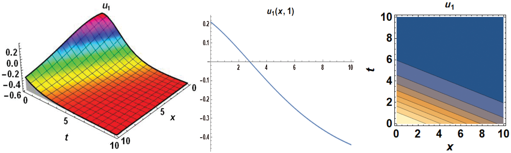
Figure 1: 3D, 2D and contour graphs respectively for w=0.5,η=2.65,q=2,k=0.2 values of Eq. (19)

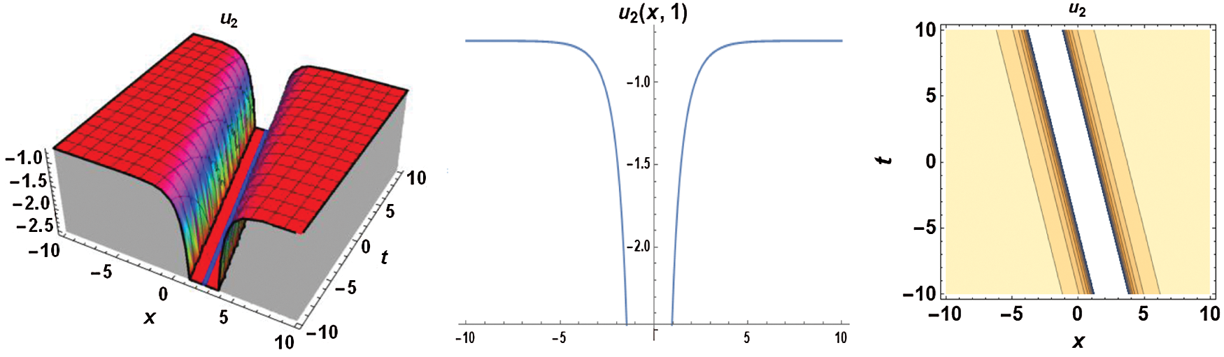
Figure 2: 3D, 2D and contour graphs respectively for w=0.5,η=0.5,q=2,k=2 values of Eq. (21)

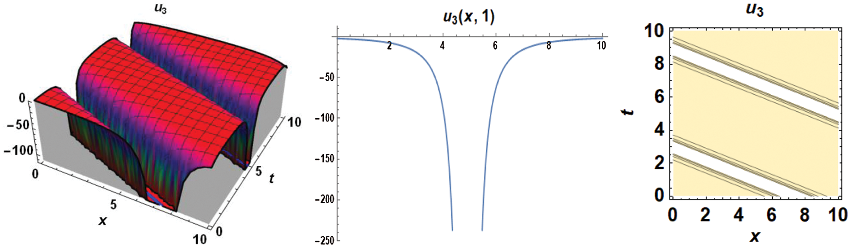
Figure 3: 3D, 2D and contour graphs respectively for w=0.5,η=2,q=2,k=0.2 values of Eq. (23)

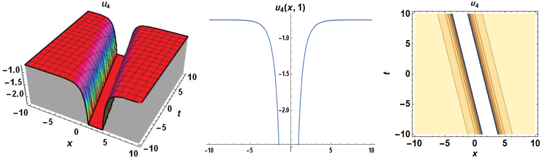
Figure 4: 3D, 2D and contour graphs respectively for w=0.5,η=0.5,q=2,k=2 values of Eq. (25)

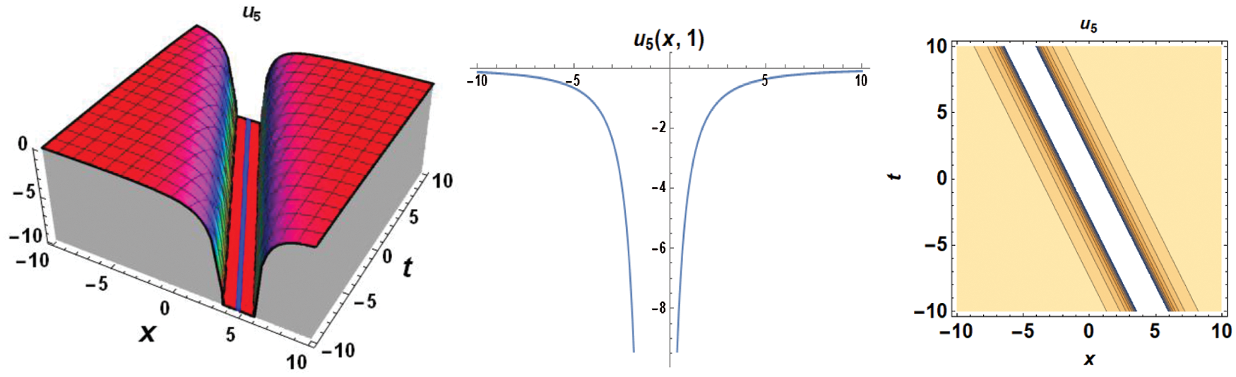
Figure 5: 3D, 2D and contour graphs respectively for r=0.5,η=0.5,q=2,k=2 values of Eq. (27)

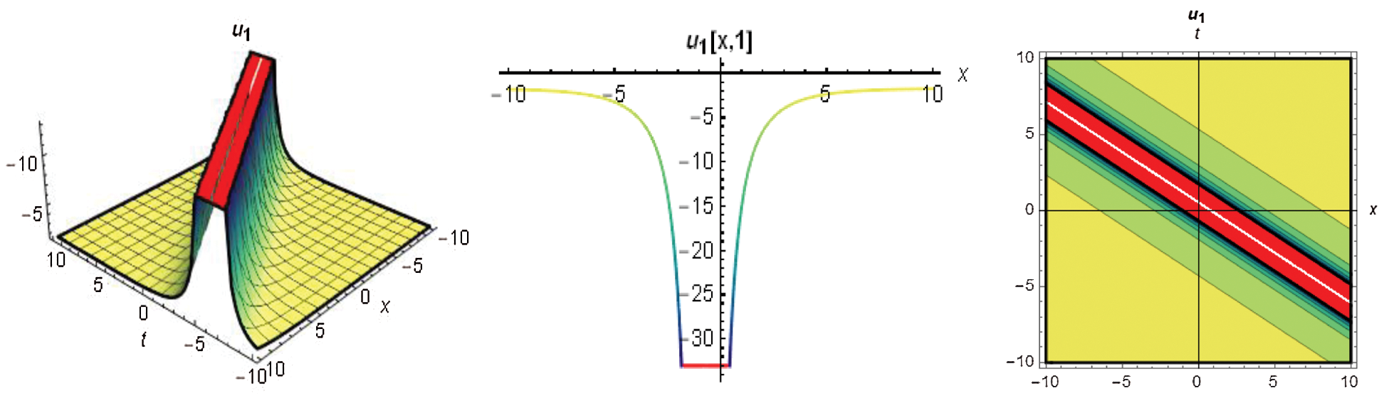
Figure 6: 3D, 2D and contour graphs respectively for c1=0.9,δ=0.3,λ=0.5,q=3,k=1,η=2 values of Eq. (31)

7  Conclusions

In this study, we have achieved hyperbolic, rational, dark soliton and trigonometric traveling wave solutions for the LWE in a magneto-electro-elastic circular rod using sub equation method and (1/G′) -expansion method. By giving arbitrary values to the constants in the solution obtained, 3D, 2D and contour graphics of the solution representing the stationary wave are presented. It has been observed that the methods used are easy, effective and powerful, and solutions of NLEEs can be obtained. It would be even more valuable to add a physical meaning to these solutions in the future. Computer package program was used in the construction of these solutions.

Funding Statement: The authors received no specific funding for this study.

Conflicts of Interest: The authors declare that they have no conflicts of interest to report regarding the present study.

This work is licensed under a Creative Commons Attribution 4.0 International License, which permits unrestricted use, distribution, and reproduction in any medium, provided the original work is properly cited.