Sound & Vibration

DOI: 10.32604/sv.2021.015938

ARTICLE

Corrected Statistical Energy Analysis Model in a Non-Reverberant Acoustic Space

Al Munawir1, Azma Putra2,*, Iwan Prasetiyo3, Wan Mohd Farid Wan Mohamad2 and Safarudin Herawan4

1Jurusan Teknik Mesin, Universitas Teuku Umar, Meulaboh, 23615, Indonesia
2Fakulti Kejuruteraan Mekanikal, Universiti Teknikal Malaysia Melaka, Melaka, 76100, Malaysia
3Acoustic Laboratory, Department of Engineering Physics, Institut Teknologi Bandung, Bandung, 40132, Indonesia
4Department of Industrial Engineering, Bina Nusantara University, Jakarta, 11480, Indonesia
*Corresponding Author: Azma Putra. Email: azma.putra@utem.edu.my
Received: 25 January 2021; Accepted: 26 May 2021

1  Introduction

Several methods exist to predict noise level inside the acoustic space such as Finite Element Analysis (FEA) and Statistical Energy Analysis (SEA). The FEA is implemented for low frequency range where distinct mode in the energy is important. The SEA is applied for high frequency range, where the energy level behaves ‘statistically’ (in which only its average value is of interest) and while the use of the FEA will be too costly. SEA have been widely used in aerospace [1], automobile and railway vehicle [2,3], ship building industry and also building acoustics [4]. In SEA, a structure is divided into subsystems, that are characterized by their modal density and damping loss factor, and the energy flow between subsystems is described using the coupling loss factor.

The coupling loss factor (CLF) and damping loss factor (DLF) are the important SEA parameters to be obtained from the SEA method apart from the identification of the weak coupling region. They determine the proportionality of the energy flows between any two SEA sub-systems and the energy absorption in each subsystem. In particular, good predictions of CLF are critically important to obtain good estimation of the noise and vibration in a system. Fahy [5] outlines two methods of calculating coupling loss factor: (1) modal approach; (2) wave approach. Modal approach is proposed based on an assumption of uncorrelated modal of two subsystems interacting to exchange energy where two reciprocal situations related to sinusoidal load and transmission coefficient are considered. On the other hand, wave approach is based on the wave transmission through each subsystem to the joints.

In practice, for multipoint coupling, the CLF and DLF can be determined either using power energy injection method [6–8], or deterministic formulation and numerical method as presented in James et al. [9,10]. Price et al. [11] formulated the CLF between room and cavity, assuming that transmission from room to cavity is the same as transmission from room to room. Mace et al. [12] predicted the coupling loss factor using SEA theory for systems consisting of rectangular plates. It is found that if the damping is large enough (weak coupling), the response is independent of the shape of the plates, while for lighter one (strong coupling) the response is dictated by the specific geometry of each plate. Ahmida et al. [13] proposed the coupling loss factor model via the Spectra Element Method (SEM). By using the SEM approach, the CLFs can be obtained for arbitrary framed structure connections.

Experimental approaches are also applicable for determining the CLF as demonstrated by Hopkins [14] who predicted the CLF for bending wave transmission between coupled plates or Cushieri et al. [15] presented a method for calculating the dissipation and CLF from SEA model of a fully assembled machinery structure. The method is based on the measurements of the total loss factors and the energy ratios between the subsystems of the machine structure when they are fully assembled. All approaches again assumed that the subsystem must have high modal overlap (reverberant energy), the condition which makes the SEA method only works for high frequency range.

A modified SEA formulation for the non-resonant response was proposed by Renji et al. [16]. The model applied different expression for the CLFs based on the sound power transmission and absorption coefficient of the structure. It was found that the non-resonant response was significant for thin light panels. Ribeiro et al. [17] developed a prediction method of the sound field inside large acoustic spaces where it is not possible to assume a uniform reverberant field due to attenuation and scattering. The method separates the direct and reverberant sound field contributions by the SEA framework using a correction to the traditional SEA equation.

In this paper, an improved SEA model in a non-reverberant acoustic space is proposed where such a condition is not ideal for the conventional SEA to be employed properly due to non-uniform modal density in a subsystem. The modelling technique is proposed by removing the direct field component from the total measured sound energy. This method has been applied in a reverberant space of a car cabin as in Putra et al. [18]. However in this paper, the model is again explained in details and experiment was conducted in a more controlled acoustic space in laboratory. The reminder of this paper is organized as follows: in Section 2, method of classical SEA and proposed SEA model for non-reverberant space are presented. Section 3 explains the experimental setup followed by Section 4 which presents the results of calculations, analysis, and validation. Finally, important findings are summarized in the conclusions.

2  Literature Review

2.1 Power Injection Method

The power injection method (PIM) is one of the techniques used to estimate the SEA parameters, namely the coupling loss factor and the damping loss factor. Fig. 1 shows a system divided into two subsystems each is injected with input power Pin. Based on the power balance principle, the input power at subsystem i is given by

Pin,i=ωηiEi+∑j=1i≠1N⁡ωηijEi−∑j=1i≠1N⁡ωηjiEj (1)

where ω is the frequency angular, E is the energy, ηi is the damping loss factor at the i-th subsystem, ηij is the coupling loss factor from the i-th to the j-th subsystem. The first term on the right-hand side of Eq. (1) is the dissipation of power in the subsystem i, while the second and third terms correspond to the flow of energy between subsystems due to coupling.

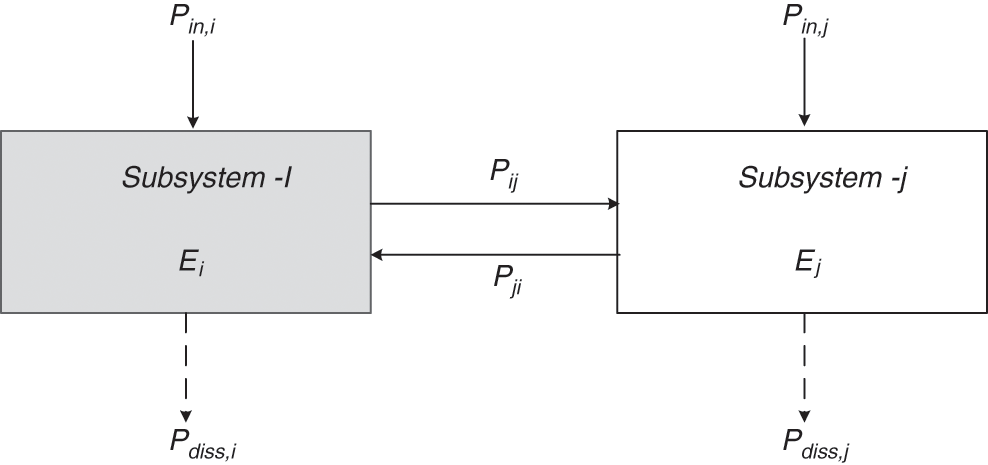
Figure 1: Schematic diagram of SEA model

Eq. (1) can be written in matrix form as

{Pin,1Pin,2}=ω[η1+η12−η21−η12η2+η21]{E1E2} (2)

If only subsystem-1 is excited over some frequency band with measured input power P1(1) , while P2 = 0, thus

{P1(1)0}=ω[η1+η12−η21−η12η2+η21]{E1(1)E2(1)} (3)

where E1(1) and E2(1) are the measured energies in each subsystem due to the injected power in subsystem-1. Now subsystem-2 is excited with the input power P1(2)

{0P2(2)}=ω[η1+η12−η21−η12η2+η21]{E1(2)E2(2)} (4)

where E1(2) and E2(2) are the measured energies due to the injected power in subsystem-2. Combining Eqs. (3) and (4) yields

[η1+η12−η21−η12η2+η21]=1ω[P1(1)00P2(2)][E1(1)E1(2)E2(1)E2(2)]−1 (5)

and therefore the SEA parameters can be obtained by

[η1+η12−η21−η12η2+η21]=1ω[P1(1)00P2(2)][E1(1)E1(2)E2(1)E2(2)]−1 (6)

The coupling loss factors are dependent on geometrical details of the connection and different wave types can be generated in structures. Relations between transmission coefficient and corresponding coupling loss factors have been derived for some common structural connections such as room to room, plate to room, plate to plate and room to plate couplings.

When coupling from room to room or room to cavity, the coupling loss factor can be calculated as [11]

η12=τ12cS4ωV (7)

where τ12 is transmission coeficient between subsystem-1 and subsystem-2, c is speed of sound in air and V is the volume in the subsystem. In room acoustics, the most common way to calculate the damping loss factor is to use the reverberation time given by

η=2.2fT60 (8)

where T60 is the reverberation time and f is the frequency. The reverberation time is defined as the time required for the energy to decrease by 60 dB from a steady state condition (after the sound source is switched off). The formula for reverberation time is given by

T60=0.16VA (9)

where A is the total absorption area in a room.

2.2 Corrected SEA Model in a Non-Reverberant Acoustic Space

In an enclosed acoustic space, the total energy of the sound field at any given location is the sum of energy from the direct field Edir radiated by the sound source and the reverberant field Erev created by the reflections

E=Edir+Erev (10)

For a room with highly reflective, non-parallel walls, for instance in a reverberant chamber, the sound field can be ‘diffuse’, where the acoustic mode in a frequency band has high modal overlap. According to Schroeder [19], this is only valid above a certain starting frequency where the frequency is proportional to the volume of the room and inversely proportional to its reverberation time.

If the walls of a room are damped with sound absorbers, the reverberation time is shorter and the ‘Schroeder frequency’ increases. The direct field component dominates wider frequency range of the total sound field. As the SEA model is based on the assumption of reverberant energy, a correction is thus important to separate the direct field component from the total energy. Under a steady-state condition, the general power balance equation in Eq. (1) for N subsystems can be expressed as

Pin,i(1−α¯i)=ωηiErev,i+∑j=1i≠1N⁡ωηijErev,i−∑j=1i≠1N⁡ωηjiErev,j (11)

where α¯i is the average absorption coefficient in the i-th subsystem and Erev,i is the reverberant field component after the removal of the direct field component from the measured energy in the corresponding subsystem. Here the term Pin,i(1−α¯i) only accounts for the loss of the power at the first reflection.

2.3 Elimination of the Direct Field Component

In Ribeiro et al. [17], the assumption was that the sound propagates spherically and the component of the direct field can be obtained an inverse formula. However, the power of the sound source must be known. In this paper, a new approach is proposed to determine the direct field component from the measured acoustic signal in the corresponding subsystem. The direct field component can be identified from the measured impulse response, h(t) where this is obtained by applying the inverse Fast Fourier Transform (FFT) to the measured frequency response function (FRF), H (ω) in the subsystem expressed as

h(t)=iFFT(H(ω)) (12)

For a sound field which is not completely reverberant (there is still a significant direct field energy), the impulse response will be indicated by an early high peak which is the direct field component, and followed by other smaller peaks, which are the reflected signals building up the reverberant energy. This direct field component can be removed from the signal by applying a unit step window function given by

w(t)={0,fort≤ta1,fort>ta (13)

where ta is the arrival time of the first reflection.

The corrected impulse response is thus given by

hc(t)=h(t)×w(t) (14)

The FRF without the direct field component can be obtained by re-applying the FFT to the corrected impulse response.

Hc(t)=FFT(hc(t)) (15)

The illustration of the methodology is shown in Fig. 2.

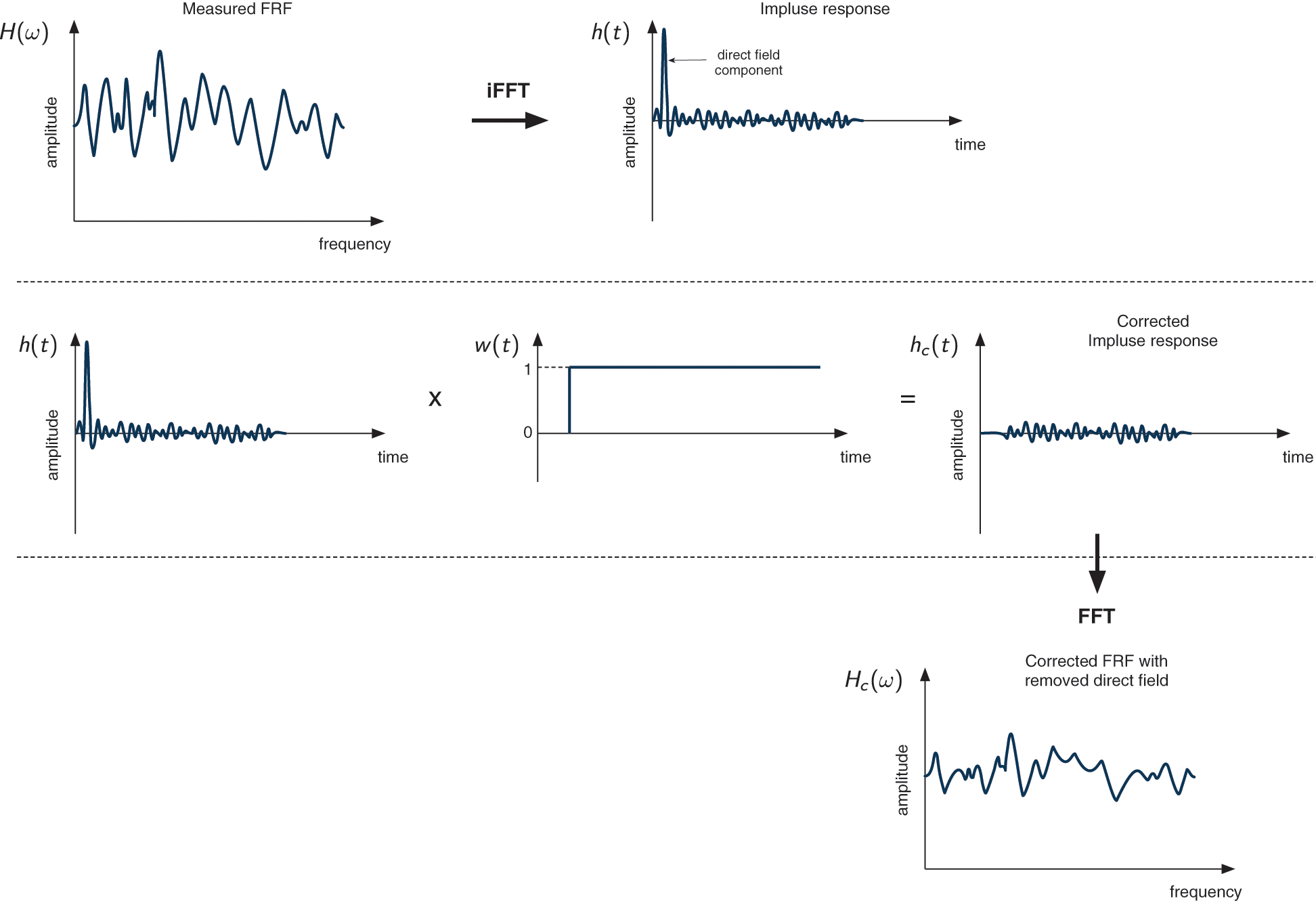
Figure 2: Diagram methodology to remove the direct field component

3  Experimental Work and Result Analysis

3.1 Experimental Subsystems

In order to validate the proposed corrected SEA model in an acoustic space, a controlled room is required to conveniently set the reverberant and non-reverberant condition. For this purpose, a coupled-box made of 1 mm mild steel plates each having volume of roughly 0.18 m3 was constructed. Each box is designed with non-parallel walls to optimize the generation of diffuse field for the reverberant condition. The boxes were separated by a solid partition made of the same panel as a coupling between the two acoustic spaces where the panel has an opening area of 150 × 150 mm at the middle. The box can be seen in Fig. 3.

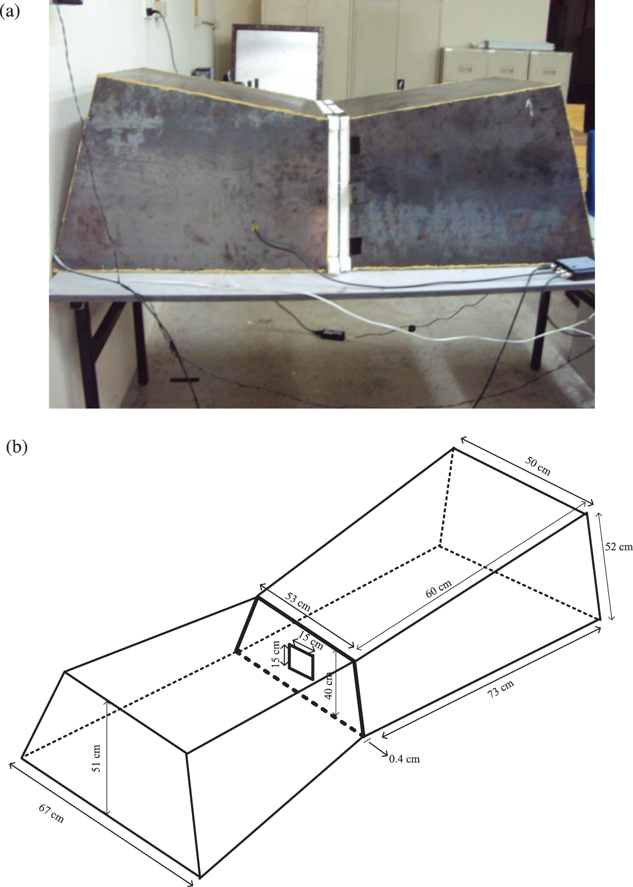
Figure 3: (a) The experimental coupled-box with two subsystems and (b) the schematic diagram of the box

The setup of the experimental SEA with the coupled-box is shown in Fig. 4. The power injection method was implemented where the room was excited by broadband white noise from the loudspeaker. The acoustic microphones then measured the sound pressure level and the data were processed by a signal analyzer.

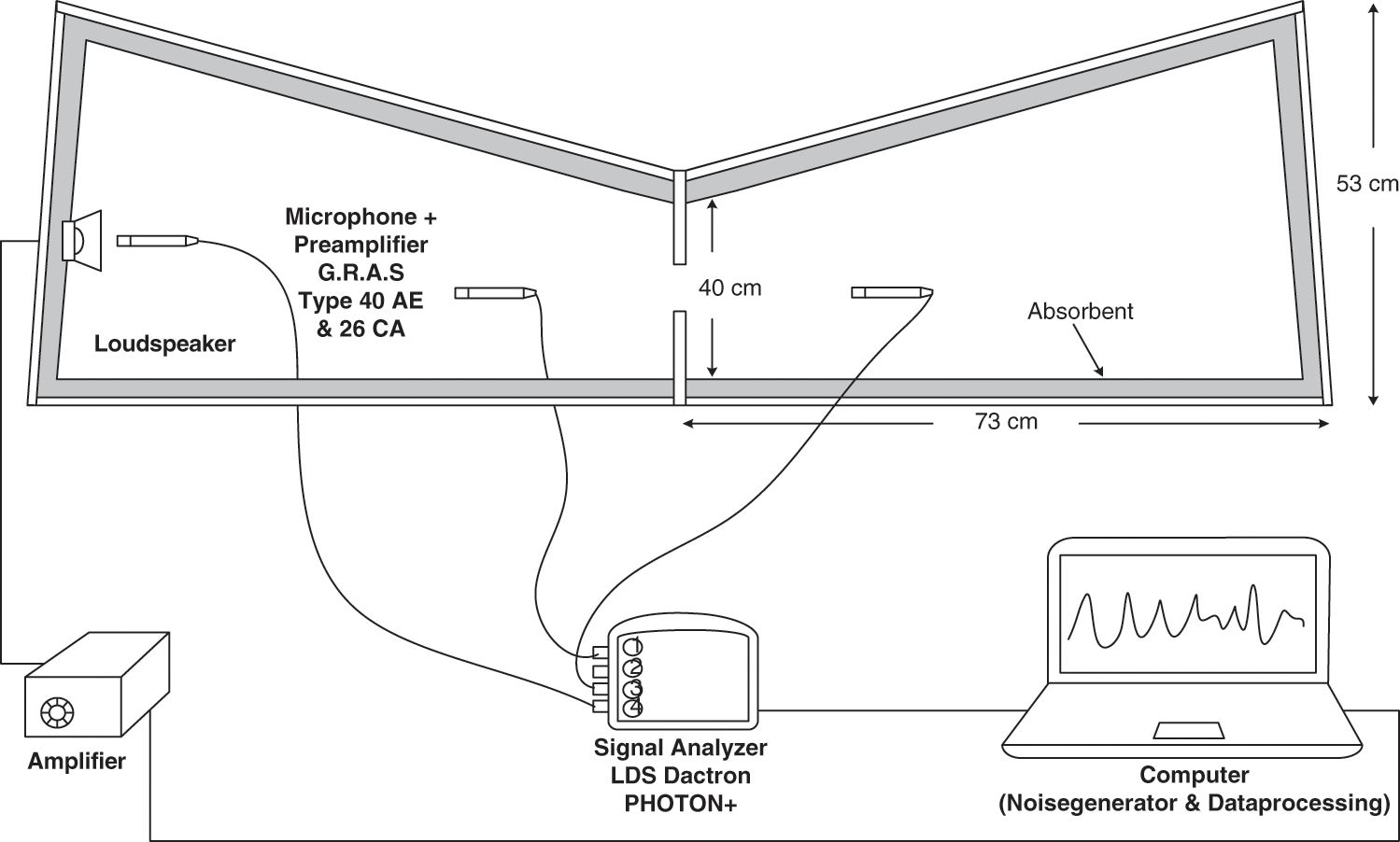
Figure 4: Measurement setup for the experimental SEA

The data was recorded as the frequency response function (FRF) between the signal from the source to that from the response point. For this purpose, the reference microphone was located in front of the loudspeaker. Assuming the system is linear, this technique eliminates the dependency of the results on the amplification of the loudspeaker and to ensure fair comparison were made among sets of experiments. The measured FRF is defined as

H(ω)=Sxx(ω)Syy(ω)|Sxy(ω)|2 (16)

where Sxx and Syy are the auto-spectra from the reference microphone and the response microphone, respectively and Sxy is the cross-spectrum between the two microphones. The response microphone was positioned in four locations in the room to obtain the spatial average of the sound pressure.

3.2 Measurement of Sound Power

The accuracy of the SEA method depends on the accuracy of the input power required in the power balance equation. The sound power measurement from the loudspeaker was therefore conducted according to BS-ISO 3746 [20] to provide good precision of measurement and good accuracy of results. The measurement was done in a semi-anechoic chamber.

The experimental setup for the sound power measurement is shown in Fig. 5. The acoustic pressure was measured over ten measurement locations forming a hemispherical surface enclosing the loudspeaker. The measurement distance between loudspeaker and each of microphone positions is 1 m. The sound power from the loudspeaker was also measured in terms of the FRF, i.e., the squared pressure measured from the response microphone normalised by the squared pressure from the reference microphone as represented in Eq. (16).

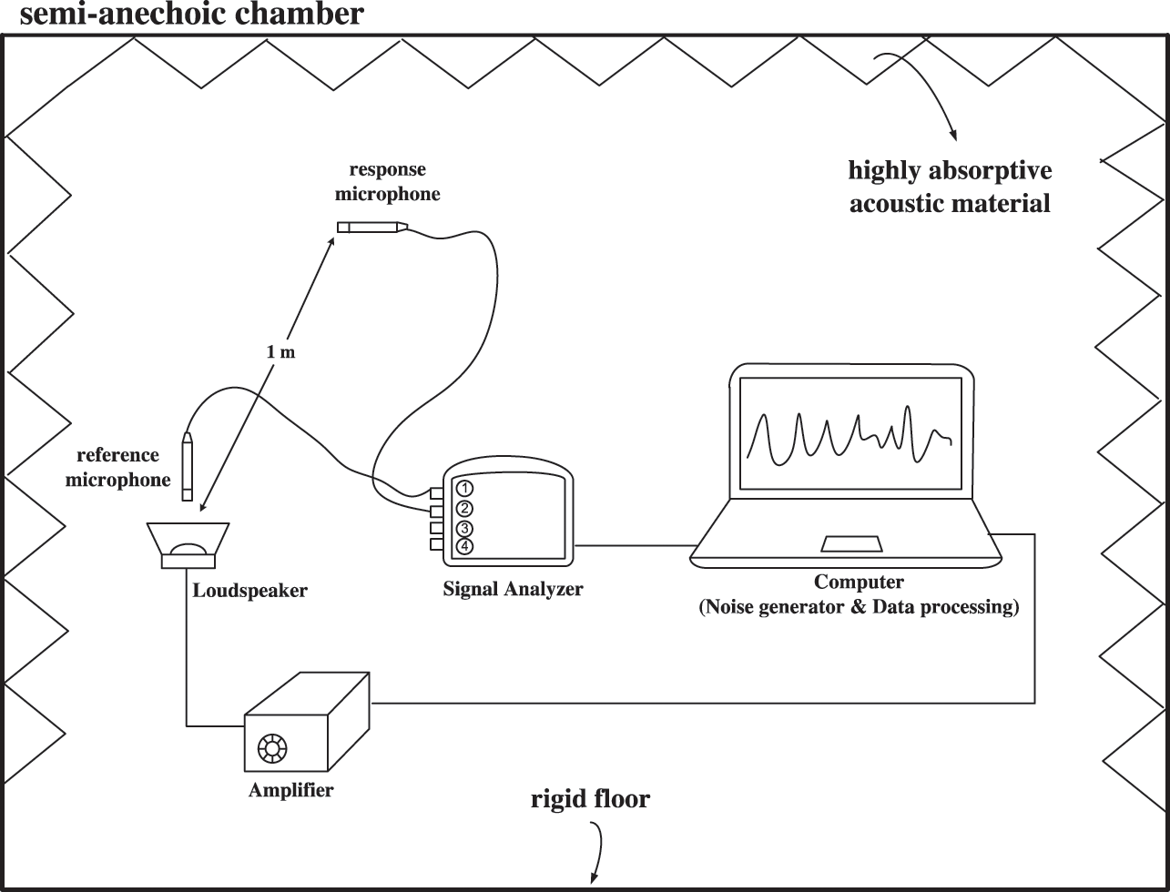
Figure 5: Experimental setup for the sound power measurement inside the semi-anechoic chamber

The equivalent ‘normalised’ sound power level is calculated by

P^(ω)=(H(ω)ρc2)×S (17)

where S=2πr2 is the area of the hemispherical surface with r is the distance of the response microphone from the loudspeaker, ρ is the density of air and c is the speed of sound.

The measured normalised sound power level in one-third octave bands can be seen in Fig. 6. It shows that the sound power is almost flat from 500 Hz to 6 kHz, which can provide sufficient injected energy for the whole corresponding frequency bands. The next section presents the estimation of the SEA parameters, namely the coupling loss factor (CLF) and damping loss factor (DLF) from the reverberation and non-reverberation conditions.

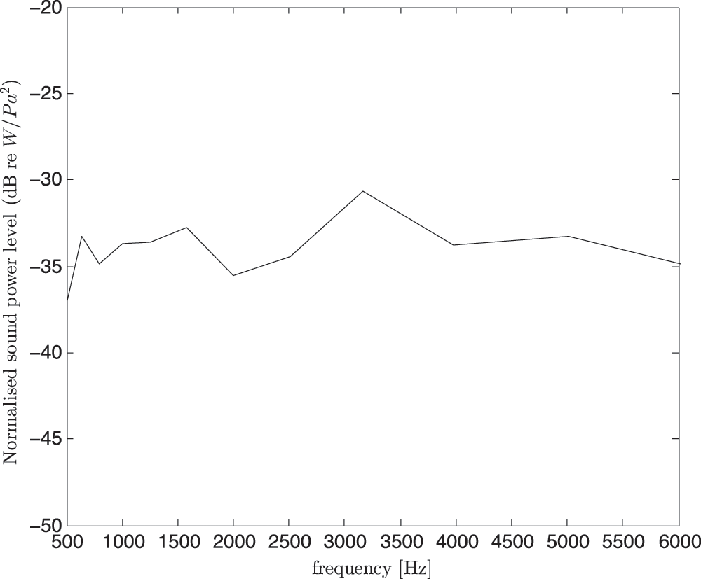
Figure 6: Measured normalised sound power from the loudspeaker

3.3 Measurement of CLF and DLF in Reverberant Condition

The determination of CLF and DLF from reverberation condition was first conducted in the coupled-box system with empty condition, that is without the presence of any absorbent materials to provide strong sound reflections (diffused field). The sound power measurement from the loudspeaker was conducted according BS-ISO 3746 [20], and the energy in the corresponding subsystem here can be considered as the normalised energy (by the squared pressure) expressed as

E^=Hi(ω)Viρc2 (18)

where Vi is the volume of subsystem i, ρ is the air density and c is the speed of sound.

Fig. 7 shows the measured impulse response where multiple peaks can be seen indicating signals reflected from the surfaces where these built up a reverberant field.

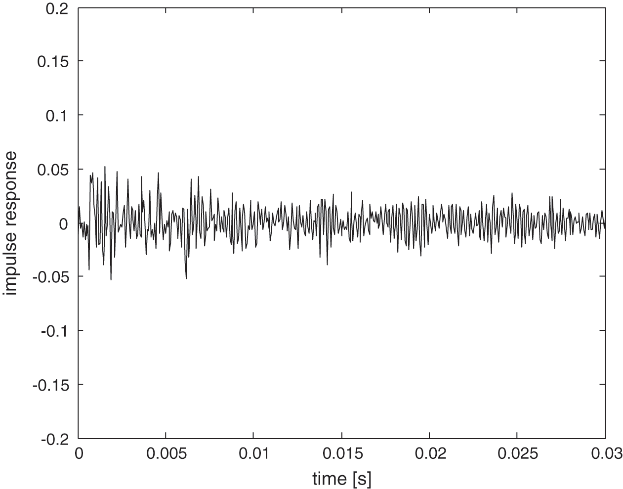
Figure 7: Measured impulse response in the reverberant condition

Fig. 8 plots the measured energy in one-third octave band in each subsystem using the power injection method mentioned in Section 2.1. The difference of energy level of roughly 3–5 dB between two subsystems can be seen as a result of some energy loss through the partition (coupling) and through dissipation.

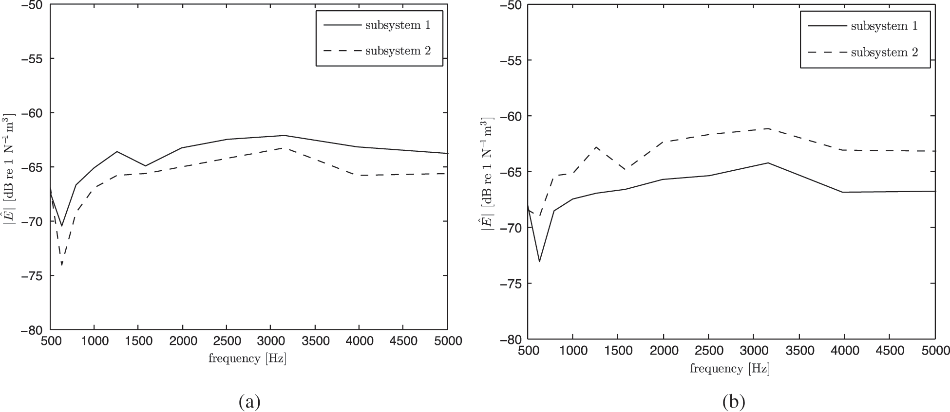
Figure 8: Measured normalised energy in the subsystems with the sound power injected in: (a) subsystem-1 and (b) subsystem-2

Fig. 9 shows the estimated CLF where good agreement with the theoretical CLF from Eq. (7) above 1.5 kHz can be seen indicating diffuse sound field above this frequency for such a small acoustic room.

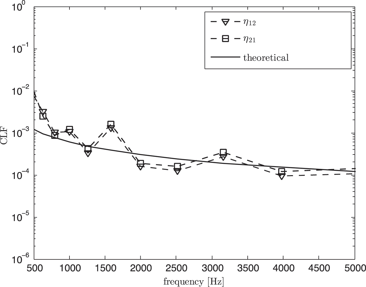
Figure 9: Coupling loss factor (CLF) obtained from experimental SEA in a reverberant condition compared with the theoretical value (Eq. (7))

Fig. 10 shows the measured DLF where good agreement with the theoretical DLF from Eq. (9) can also be seen above 1.5 kHz. The reverberation time required to calculate the theoretical DLF was measured using dBsolo sound analyzer type SWT001. Large discrepancy below 1.5 kHz might be due to the inaccuracy when measuring the reverberant time for low frequency at a relatively small space.

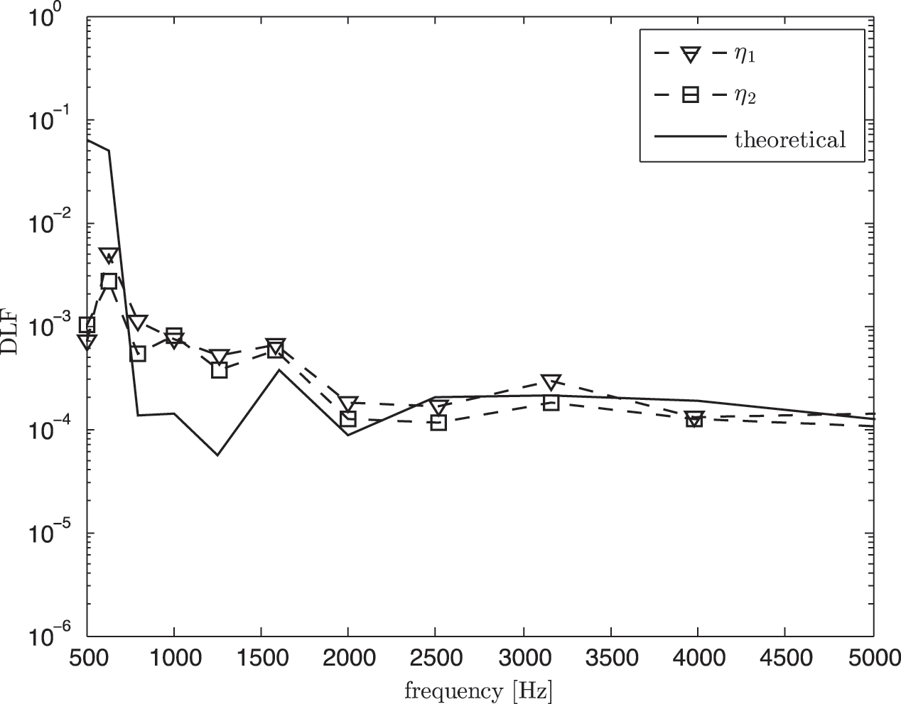
Figure 10: Damping loss factor (DLF) from experimental SEA in a reverberant condition compared with the theoretical value (Eq. (8))

3.4 Measurement of CLF and DLF in the Non-Reverberant Condition

In order to realize the non-reverberant condition, absorbent materials made of sponge were now installed on the inner room surfaces for both subsystems (see Fig. 11) except on the partition. The absorption coefficient of the sponge was measured using the transfer function method in an impedance tube according to BS-ISO 10534 [21].

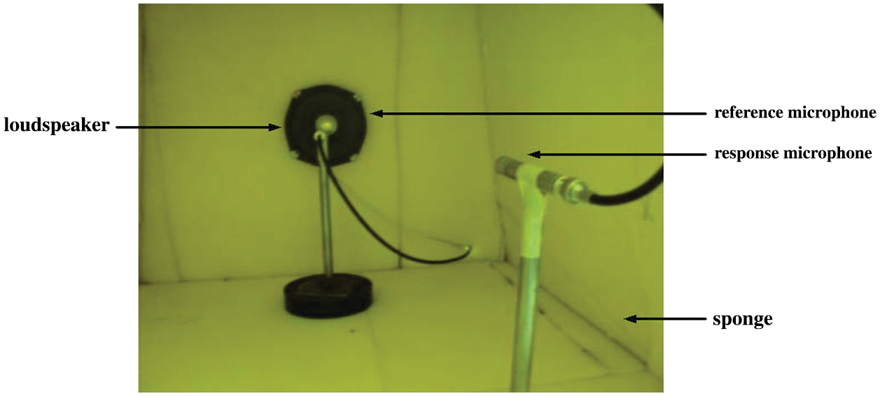
Figure 11: Arrangement of experimental SEA in the non-reverberant condition with sound absorbent attached on the wall

Fig. 12 shows the normalised energy in the injected subsystem before and after the presence of the sound absorber. It can be seen that the energy was suppressed by almost 10 dB due to the dissipation of sound energy by the absorbent.

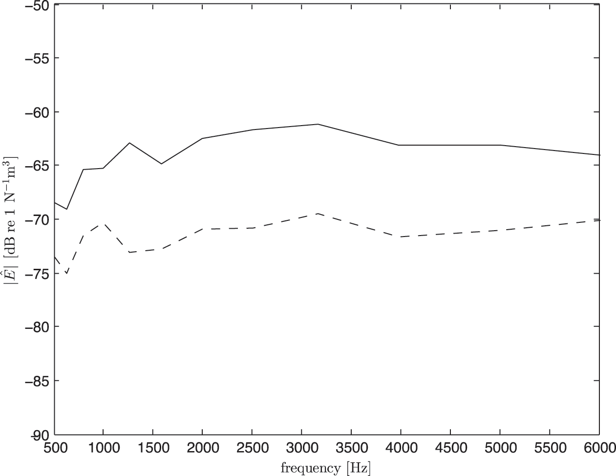
Figure 12: Measured impulse response in the non-reverberant after removing the direct field component

Fig. 13 shows the measured impulse response in the box from the non-reverberant condition. Compared to the result from Fig. 5, the direct field component here now is clearly seen by a single distinct peak signal almost at the initial time at around t = 0.001 s. Using the windowing process (see again Fig. 2), this direct field component was removed as shown in Fig. 14.

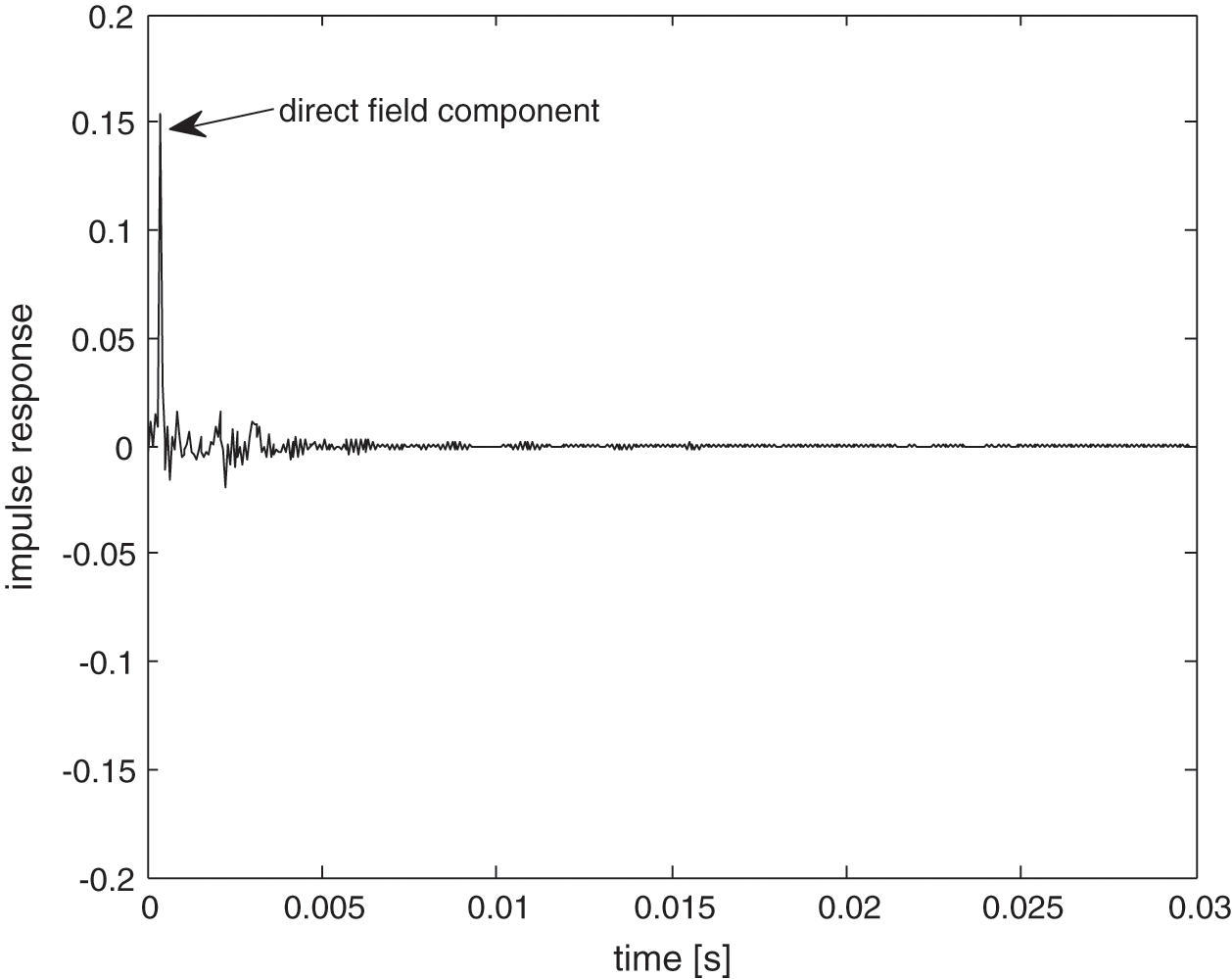
Figure 13: Measured impulse response in the non-reverberant condition

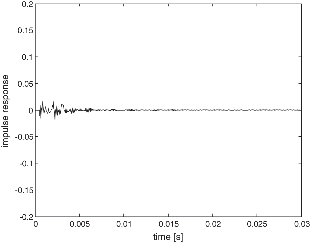
Figure 14: Measured impulse response in the non-reverberant after removing the direct field component

Fig. 15 presents the energy level before and after direct field correction were performed where difference of nearly 5 dB indicates that the direct field component significantly contributes to the total sound field.

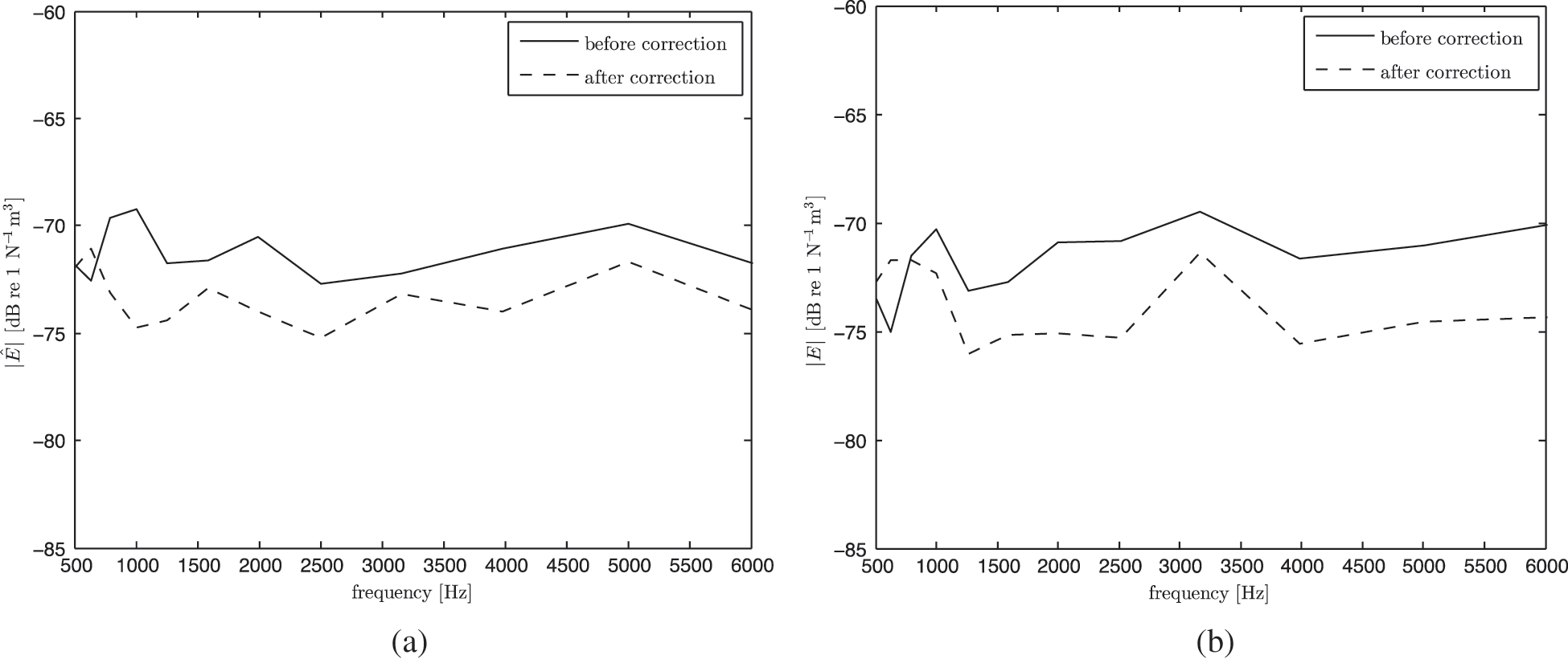
Figure 15: Measured normalised energy in the subsystems with the sound power injected in: (a) subsystem-1 and (b) subsystem-2 before and after removing the direct field component

Fig. 16 shows the coupling loss factor obtained using the classical SEA model in Eq. (6), that is before removing direct field component. It can be seen that the measured CLF overestimates the theory. By using the corrected SEA model in Eq. (11), the results as seen in Fig. 17 now have better agreement with the theoretical CLFs at high frequency above 1.5 kHz.

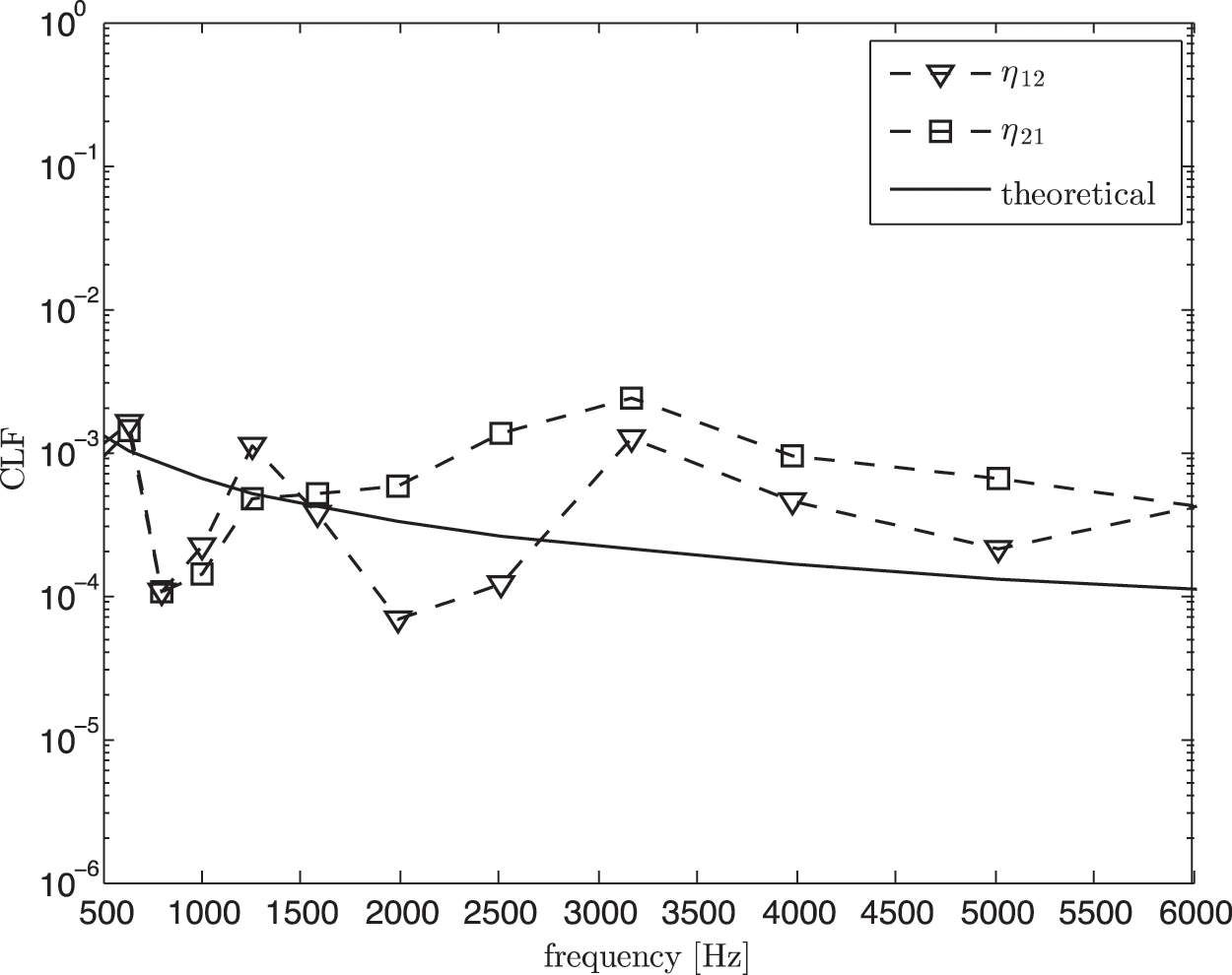
Figure 16: Coupling loss factor (CLF) from experimental SEA in non-reverberant condition before removing the direct field component (classical SEA model) compared with the theoretical value (Eq. (7))

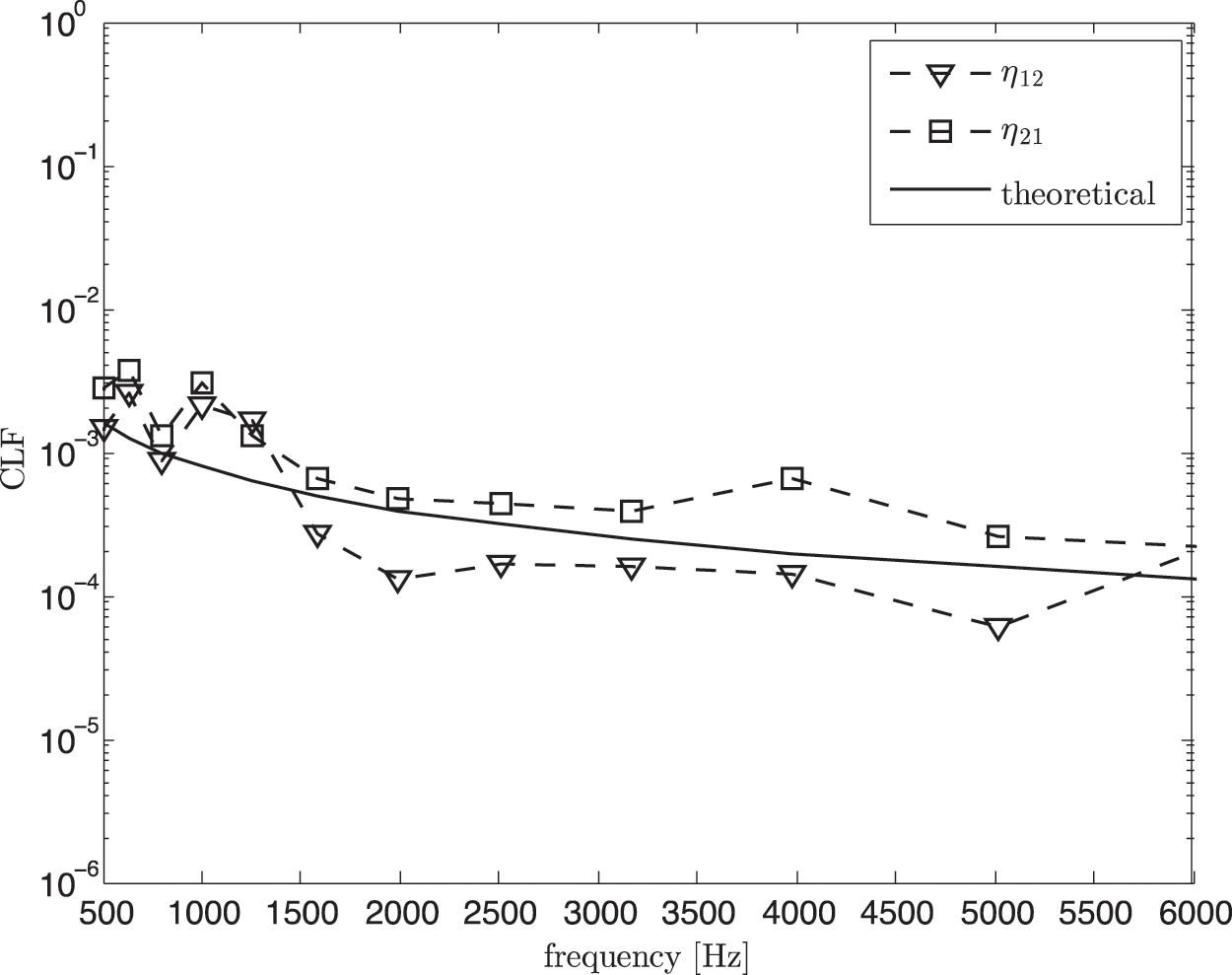
Figure 17: Coupling loss factor (CLF) from experimental SEA in non-reverberant condition after removing the direct field component (corrected SEA model) compared with the theoretical value (Eq. (7))

Fig. 18 shows the damping loss factor from the classical SEA model which can also be seen to overestimate the theory due to the domination of the direct field component. After removing the direct field component, again good agreement is obtained as seen in Fig. 19 between the estimated DLF and the theory at high frequency above 1.5 kHz. Same as the results in Fig. 10, the theoretical DLF was calculated using Eq. (8).

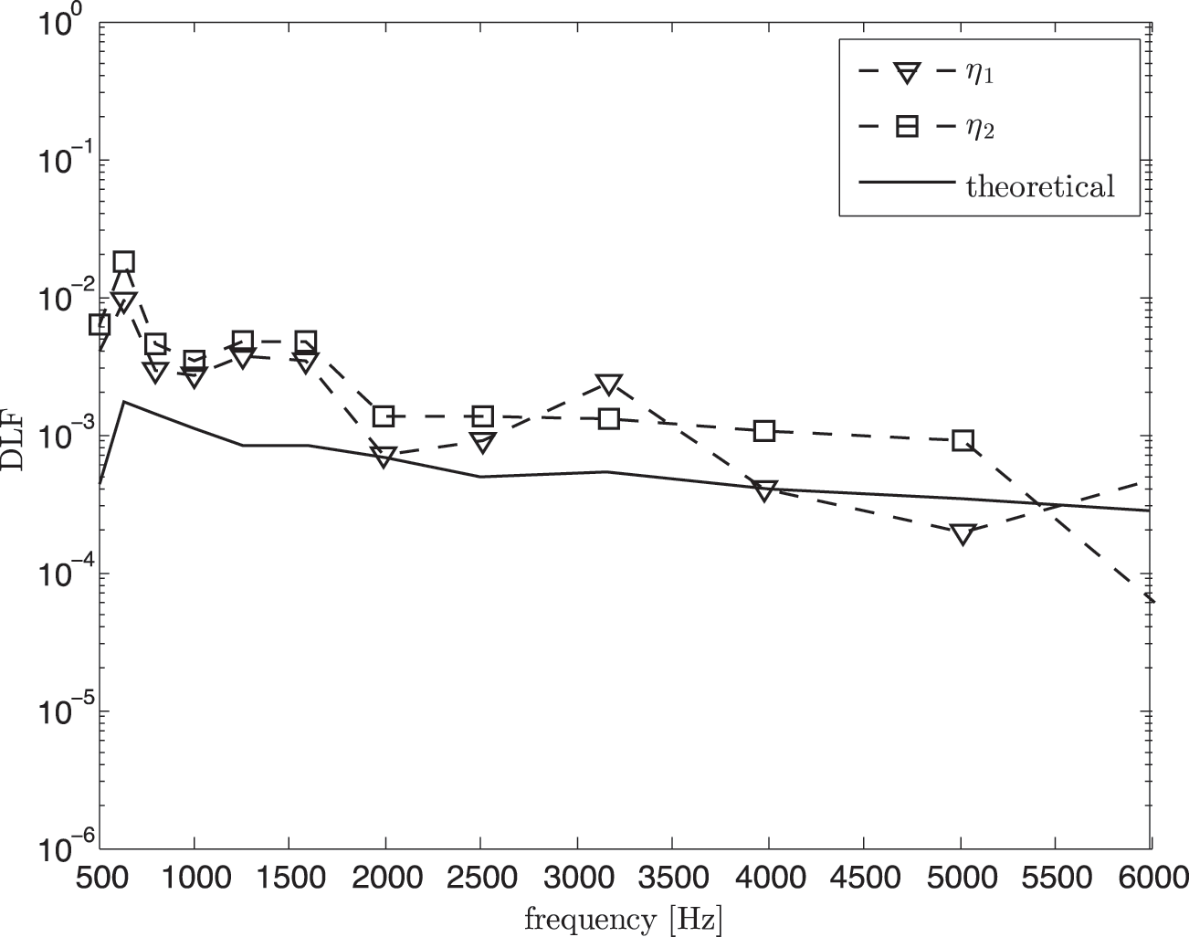
Figure 18: Damping loss factor (DLF) from experimental SEA in non-reverberant condition before removing the direct field component (classical SEA model) compared with the theoretical value (Eq. (8))

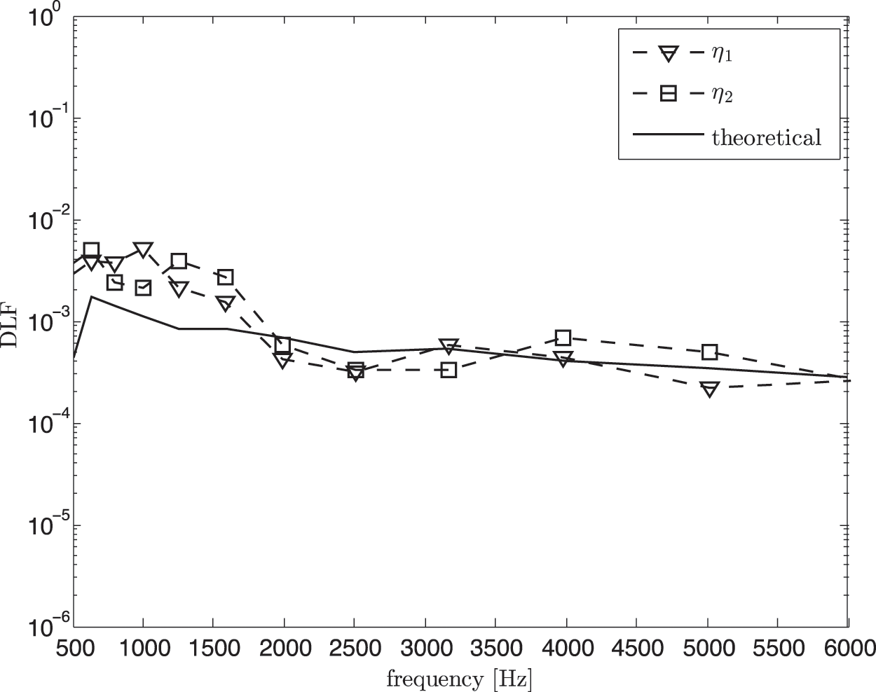
Figure 19: Damping loss factor (DLF) from experimental SEA in non-reverberant condition after removing the direct field component (corrected SEA model) compared with the theoretical value (Eq. (8))

4  Conclusion

A new approach in the SEA modelling has been proposed to solve problem in a non-reverberant acoustic space, where direct field component is dominant in the energy of a subsystem. The model eliminates the direct field component from the total sound energy and the classical SEA equation is modified to account only the reverberant components. The model is validated through an experimental SEA in a controlled environment in a steel box with two rooms. The results show that the corrected SEA model give more accurate SEA parameters (coupling loss factors and damping loss factors) to the theoretical values. This corrected SEA model can be applied in an acoustic space where the presence of absorbing materials may prevent the reverberant condition and thus use of classical SEA may not be valid, such as car cabin, airplane cabin, small room with acoustic materials, and large room. The model can be extended to be used for prediction of noise level radiated from a vibrating panel to a non-reverberant acoustic space.

Funding Statement: The authors gratefully acknowledge the financial support provided for this project by the Ministry of Higher Education Malaysia (MoHE) under Fundamental Research Grant Scheme No. FRGS/1/2016/FTK-CARE/F00323.

Conflicts of Interest: The authors declare that they have no conflicts of interest to report regarding the present study.

References

 1.  Petrone, G., Melillo, G., Laudiero, A., De Rosa, S. (2019). A Statistical Energy Analysis (SEA) model of a fuselage section for the prediction of the internal Sound Pressure Level (SPL) at cruise flight conditions. Aerospace Science and Technology, 88, 340–349. [Google Scholar]

 2.  Lee, H. R., Kim, H. Y., Jeon, H. J. (2019). Application of global sensitivity analysis to statistical energy analysis: Vehicle model development and transmission path contribution. Applied Acoustics, 146, 368–389. [Google Scholar]

 3.  Forssén, J., Tober, S., Frid, A. (2012). Modelling the interior sound field of a railway vehicle using statistical energy analysis. Applied Acoustics, 73(4), 307–311. [Google Scholar]

 4.  Jang, H., Hopkins, C. (2018). Prediction of sound transmission in long spaces using ray tracing and experimental Statistical Energy Analysis. Applied Acoustics, 130, 15–33. [Google Scholar]

 5.  Fahy, F. J. (1994). Statistical energy analysis: A critical overview. Philosophical Transactions of the Royal Society of London. Series A: Physical and Engineering Sciences, 346(1681), 431–447. [Google Scholar]

 6.  Fung, A. K., Davis, E. B. (2005). Prediction of airplane aft-cabin noise using statistical energy analysis. Journal of the Acoustical Society of America, 118(3), 1847. [Google Scholar]

 7.  Cacciolati, C., Guyader, J. I. (1994). Measurement of SEA coupling loss factors using point mobilities. Philosophical Transactions of the Royal Society of London. Series A: Physical and Engineering Sciences, 346(1681), 465–475. [Google Scholar]

 8.  Thite, A. N., Mace, B. R. (2007). Robust estimation of coupling loss factors from finite element analysis. Journal of Sound and Vibration, 303(3), 814–831. [Google Scholar]

 9.  James, P. P., Fahy, F. J. (2000). A modal interaction indicator for qualifying cs an indicator of strength of coupling between SEA subsystems. Journal of Sound and Vibration, 235(3), 451–475. [Google Scholar]

10. Craik, R. J. M. (2003). Non-resonant sound transmission through double walls using statistical energy analysis. Applied Acoustics, 64(3), 325–341. [Google Scholar]

11. Price, A. J., Crocker, M. J. (1970). Sound transmission through double panels using statistical energy analysis. Journal of the Acoustical Society of America, 47(3A), 683–693. [Google Scholar]

12. Mace, B. R., Rosenberg, J. (1998). The SEA of two coupled plates: An investigation into the effects of subsystems irregularity. Journal of Sound and Vibration, 212(3), 395–415. [Google Scholar]

13. Ahmida, K. M., Arruda, J. R. F. (2003). Estimation of the SEA coupling loss factors by means of spectral element modeling. Journal of the Brazilian Society of Mechanical Sciences and Engineering, 25, 259–263. [Google Scholar]

14. Hopkins, C. (2009). Experimental statistical energy analysis of coupled plates with wave conversion at the junction. Journal of Sound and Vibration, 322(1), 155–166. [Google Scholar]

15. Cushieri, J. M., Sun, J. C. (1994). Use the statistical energy analysis for rotaring machinery, Part I: Determination of dissipation and coupling loss factors using energy ratios. Journal of Sound and Vibration, 170, 181–190. [Google Scholar]

16. Renji, K., Nair, P. S., Narayanan, S. (2001). Non-resonant respons using statical energy analysis. Journal of Sound and Vibration, 241(2), 253–270. [Google Scholar]

17. Ribeiro, R., Smith, M. (2005). Use of SEA to model the sound filed in large acoustic spaces. Forum Acousticum, pp. 79–84. Budapest. [Google Scholar]

18. Putra, A., Munawir, A., Farid, W. M. (2015). Corrected statistical energy analysis model for car interior noise. Advances in Mechanical Engineering, 7(1). DOI 10.1155/2014/304283. [Google Scholar] [CrossRef]

19. Schroeder, M. R. (1996). The “Schroeder frequency” revisited. Journal of the Acoustical Society of America, 99(5), 3240–3241. [Google Scholar]

20. ISO, Standard ISO 3746 Acoustics (2010). Determination of sound power levels and sound energy levels of noise sources using sound pressure—Survey method using an enveloping measurement surface over a reflecting plane. [Google Scholar]

21. ISO, Standard 10534–2 Acoustics (1998). Determination of sound absorption coefficient and impedance in impedance tubes–transfer function method. [Google Scholar]

This work is licensed under a Creative Commons Attribution 4.0 International License, which permits unrestricted use, distribution, and reproduction in any medium, provided the original work is properly cited.