Sound & Vibration

DOI: 10.32604/sv.2021.014445

ARTICLE

He’s Homotopy Perturbation Method and Fractional Complex Transform for Analysis Time Fractional Fornberg-Whitham Equation

Yanni Zhang1,2 and Jing Pang1,2,*

1College of Science, Inner Mongolia University of Technology, Hohhot, 010000, China
2Inner Mongolia Key Laboratory of Statistical Analysis Theory for Life Data and Neural Network Modeling, Inner Mongolia University of Technology, Hohhot, 010000, China
*Corresponding Author: Jing Pang. Email: pang_j@imut.edu.cn
Received: 28 September 2020; Accepted: 18 June 2021

1  Introduction

Over the last few years, the study of the fractional calculus and applications in the area of life science, physics and the engineering has been paid a great attention. The fractional calculus are also used in many other fields, such as optics, solitary waves, control theory of dynamical systems, and so on, which can be derived by linear or nonlinear fractional order differential equations. Recently, the studies of nonlinear problems and their effects are of widely significance. Many analytical and approximation methods have been presented to solve nonlinear fractional differential equations such as [1–11]. The homotopy perturbation method (HPM) [12–14] is widely applied to various science and engineering problems. This method was first proposed by He [12]. Fractional complex transform was suggested also by He et al. [15–19], which converts the fractional differential equation into its equivalent differential equation, so that the HPM can be effectively used. Now it is considered as a powerful method to find the approximation solutions of nonlinear fractional order differential equations.

In this paper, we study the time fractional Fornberg-Whitham (FW) equation [20] as follows:

∂βu∂tβ−∂3u∂x2∂t+∂u∂x=u∂3u∂x3−u∂u∂x+3∂u∂x∂2u∂x2t>0,0<β≤1 (1)

with the initial condition:

u0(x,0)=ex2 (2)

here β is the fractal dimensions of the fractal medium and ∂β∂tβ is He’s fractional derivative defined [21–23]:

∂βu∂tβ=1Γ(n−β)dndtn∫t0t(s−t)n−β−1[u0(s)−u(s)]ds (3)

where u0(x,t) is the solution of its starting point of the nonlinear fractional order model. When β=1 , Eq. (1) becomes to be the original Fornberg-Whitham (FW) model which is a significant mathematical equation in mathematical physics. This equation was presented by Parkes et al. [24–26] in 1978 which describes nonlinear water waves with peakon solutions. The peakon solution is a special solitary wave solution which is peaked in the limiting case. The FW equation has been found to require peakon results as a simulation for limiting wave heights as well as the frequency of wave breaks. Now many scholars have researched the FW model for the fractional-order derivative because of its fractional calculus applications.

2  HPM Procedure

To illustrate the basic ideas of this method [27–32], we consider the following nonlinear functional equation:

A(u)−f(r)=0,r∈Ω (4)

with the following boundary conditions:

B(u−∂u∂n)=0,r∈Λ (5)

where A is a general functional operator, B is a boundary operator, f(r) is a known analytical function, and Λ is the boundary of the domain Ω . The operator A can be decomposed into two operators L and N , where L is linear, and N is nonlinear operator. Eq. (4) can be written as follows:

L(u)+N(u)−f(r)=0 (6)

Using the homotopy technique, we construct a following homotopy:

H(ξ,p)=(1−p)[L(v)−L(u0)]+p[A(v)−f(r)]=0p∈[0,1],r∈Ω (7)

where the homotopy parameter p is considered as a small parameter.

Obviously, we can get:

H(ξ,1)=A(ξ)−f(r) (8)

The HPM uses embedding parameter p as an expanding parameter, and basic assumption is that the solution of Eq. (6) can be specified as a power series in p :

ξ=ξ0+pξ1+p2ξ2+p3ξ3+… (9)

When p→1 , the approximate solution of Eq. (1):

u=limp→1⁡ξ=ξ0+ξ1+ξ2+ξ3+… (10)

3  HPM Implementation

According to the HPM, the first step is to transform the fractional model equation into its equivalent differential equation:

y=tβΓ(1+β) (11)

Eq. (1) can be written into its equivalent differential equation form:

∂u∂y−∂3u∂x2∂y+∂u∂x−u∂3u∂x3+u∂u∂x−3∂u∂x∂2u∂x2=0 (12)

Applying the HPM process, substituting Eq. (11) into Eq. (7), we have a set of equations that is to be simultaneously solved:

∂u0∂y−ex2=0,u0(x,0)=ex2 (13)

∂u1∂y−∂3u0∂x2∂y+∂u0∂x−u0∂3u0∂x3+u0∂u0∂x−3∂u0∂x∂2u0∂x2=0,u1(x,0)=0 (14)

−3∂u1∂x∂2u0∂x2=0,u2(x,0)=0 (15)

−3∂u1∂x∂2u1∂x2−3∂u2∂x∂2u0∂x2=0,u3(x,0)=0 (16)

We can get a solution for the Eqs. (13)–(16) in the form:

u0(x,y)=ex2(y+1) (17)

u1(x,y)=−ex2(14y+14y2) (18)

u2(x,y)=ex2(124y3−116y) (19)

u3(x,y)=−ex2(1192y4−196y3−164y2+164y) (20)

Proceeding in the above manner, the rest of the components can be obtained. Thus we got the approximate solution which has the following form:

uapprox(x,y)=ex2(1+4364y−1564y2+596y3−1192y4+…) (21)

Substituting Eq. (11) in Eq. (21) , we get:

uapprox(x,t)=ex2(1.3pc1+4364[tβΓ(1+β)]−1564[tβΓ(1+β)]2++596[tβΓ(1+β)]3−1192[tβΓ(1+β)]4+…) (22)

4  Numerical Results and Discussion

The exact result [20] of Eq. (1):

u(x,t)=e(x2−23t) (23)

In Figs. 1 and 2, the approximate solution obtained by fractional complex transform and HPM and actual solution of Eq. (1) are plotted. It is observed that HPM solutions are in closed contact with the exact solution. In Figs. 3 and 4, the solutions of Eq. (1) at various fractional-order of the derivatives are plotted which showns that the balancing phenomena between dispersion and nonlinearity is valid.

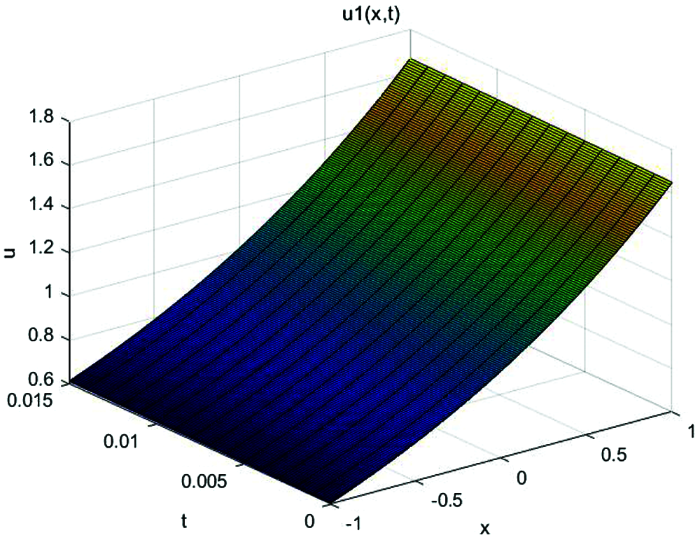
Figure 1: Approximate solution of Eq. (1) for β=1

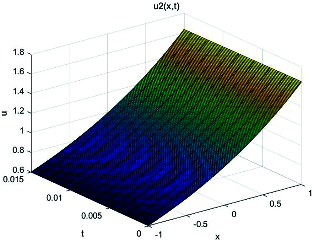
Figure 2: Exact solution of Eq. (1) for β=1

Figure 3: Approximate solution of Eq. (1) for β=0.8

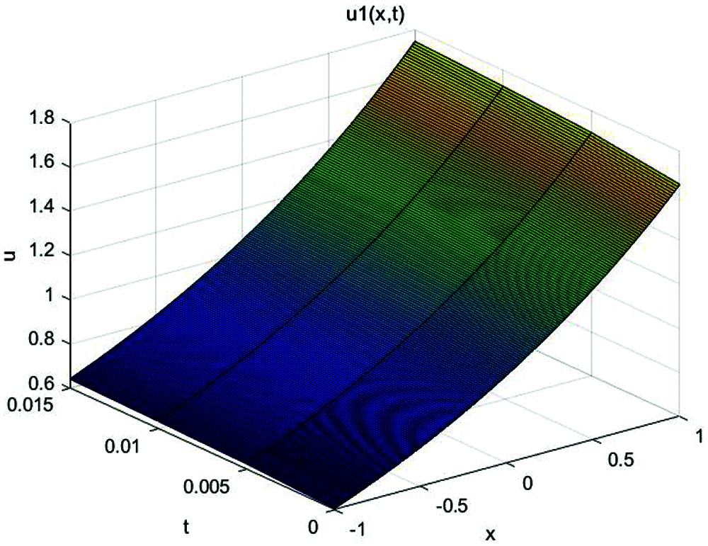
Figure 4: Approximate solution of Eq. (1) for β=0.6

In Figs. 5 and 6, the the approximate solutions of Eq. (1) at different fractional order of the derivatives are plotted. This behavior illustrated that there is directly relationship between both the width and the height of the solitary wave and the value of β . We can change the shape of solitary wave with the help of adjusting the value of fractal order β are plotted. In Figs. 7 and 8, the numerical results illustrated which confirms the high accuracy of the method.

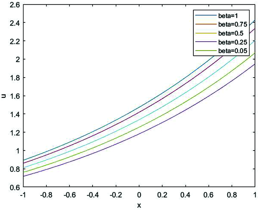
Figure 5: The relationship between β and amplitude of Eq. (1) for t=0.3

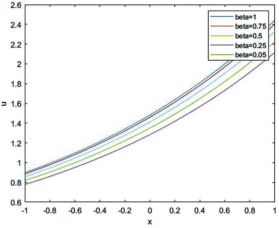
Figure 6: The relationship between β and amplitude of Eq. (1) for t=0.5

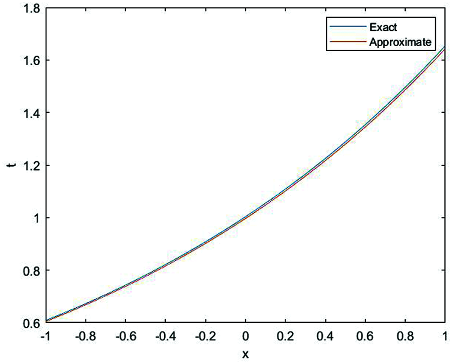
Figure 7: The relationship between exact solution (blue) and approximate solution (red) of Eq. (1) for β=1 , t=0.005

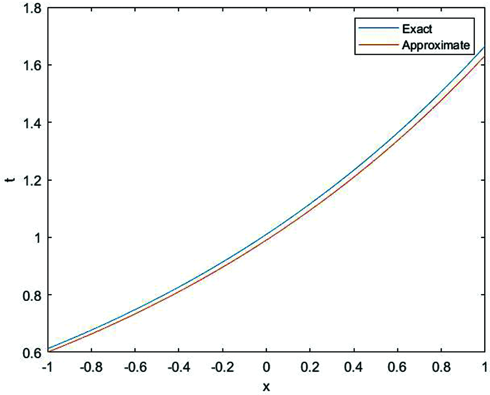
Figure 8: The relationship between exact solution and approximate solution (red) of Eq. (1) for β=1 , t=0.015

5  Conclusion

In this manuscript, a mathematical technology is used to find the solution of time fractional Fornberg-Whitham equation. The fractional-derivatives are discussed within He’s fractional derivative. The solutions are determined for fractional-order problems which shows the high accuracy and efficiency. This is easy and can be extended to other nonlinear differential equations with fractal derivatives in science and engineering.

Funding Statement: The work was supported by the National Natural Science Foundation of China under Grant No. 11561051.

Conflicts of Interest: The authors declare that we have no conflicts of interest to report regarding the present study.

References

 1.  He, J. H., Ji, F. Y. (2019). Taylor series solution for Lane-Emden equation. Journal of Mathematical Chemistry, 57(8), 1932–1934. DOI 10.1007/s10910-019-01048-7. [Google Scholar] [CrossRef]

 2.  He, J. H. (2019). The simplest approach to nonlinear oscillators. Results in Physics, 15(1), 102546. DOI 10.1016/j.rinp.2019.102546. [Google Scholar] [CrossRef]

 3.  Wang, Y., An, Y., Wang, X. Q. (2019). A variational formulation for anisotropic wave traveling in a porous medium. Fractals–An Interdisciplinary Journal on the Complex Geometry of Nature, 27(4), 1950047. DOI 10.1142/S0218348X19500476. [Google Scholar] [CrossRef]

 4.  Wang, K. L., He, C. H. (2019). A remark on Wang’s fractal variational principle. Fractals-an Interdisciplinary Journal on the Complex Geometry of Nature, 27(8), 1950134. DOI 10.1142/S0218348X19501342. [Google Scholar] [CrossRef]

 5.  He, C. H., Shen, Y., Ji, F. Y., He, J. H. (2019). Taylor series solution for fractal bratu-type equation arising in electrospinning process. Fractals–An Interdisciplinary Journal on the Complex Geometry of Nature, 28(1), 2050011. [Google Scholar]

 6.  He, J. H. (2020). Taylor series solution for a third order boundary value problem arising in architectural engineering. Ain Shams Engineering Journal, 11(4), 1411–1414. DOI 10.1016/j.asej.2020.01.016. [Google Scholar] [CrossRef]

 7.  Ahmad, H. (2019). Variational iteration algorithmi with an auxiliary parameter for wave-like vibration equations. Journal of Low Frequency Noise Vibration and Active Control, 38(3–4), 1113–1124. DOI 10.1177/1461348418823126. [Google Scholar] [CrossRef]

 8.  Ahmad, H., Seadawy, A. R., Khan, T. A., Thounthong, P. (2020). Analytic approximate solutions for some nonlinear parabolic dynamical wave equations. Journal of Taibah University for Science, 14(1), 346–358. DOI 10.1080/16583655.2020.1741943. [Google Scholar] [CrossRef]

 9.  He, J. H. (2021). A modified Li-He’s variational principle for plasma. International Journal of Numerical Methods for Heat and Fluid Flow (ahead-of-print). [Google Scholar]

10. He, J. H. (2019). Lagrange crisis and generalized variational principle for 3-D unsteady flow. International Journal of Numerical Methods for Heat and Fluid Flow, 30(3), 1189–1196. DOI 10.1108/HFF-07-2019-0577. [Google Scholar] [CrossRef]

11. He, J. H., Sun, C. (2019). A variational principle for a thin film equation. Journal of Mathematical Chemistry, 57(5), 2075–2081. DOI 10.1007/s10910-019-01063-8. [Google Scholar] [CrossRef]

12. He, J. H. (1999). Homotopy perturbation technique. Computer Methods in Applied Mechanics and Engineering, 178(3–4), 257–262. DOI 10.1016/S0045-7825(99)00018-3. [Google Scholar] [CrossRef]

13. He, J. H. (2000). A coupling method of a homotopy technique and a perturbation technique for non-linear problems. International Journal of Non-Linear Mechanics, 35(1), 37–43. DOI 10.1016/S0020-7462(98)00085-7. [Google Scholar] [CrossRef]

14. He, J. H. (2005). Application of homotopy perturbation method to non-linear wave equation. Chaos Solitons Fractals, 26(3), 695–700. DOI 10.1016/j.chaos.2005.03.006. [Google Scholar] [CrossRef]

15. He, J. H., Li, Z. B. (2012). Converting fractional differential equations into partial differential equations. Thermal Science, 1(2), 331–334. DOI 10.2298/TSCI110503068H. [Google Scholar] [CrossRef]

16. Li, Z. B., He, J. H. (2010). Fractional complex transform for fractional differential equations. Mathematical and Computational Applications, 15(5), 970–973. DOI 10.3390/mca15050970. [Google Scholar] [CrossRef]

17. Li, Z. B., Zhu, W. H., He, J. H. (2012). Exact solutions of time fractional heat conduction equation by the fractional complex transform. Thermal Science, 16(2), 335–338. DOI 10.2298/TSCI110503069L. [Google Scholar] [CrossRef]

18. Ain, Q. T., He, J. H. (2019). On two-scale dimension and its applications. Thermal Science, 23(3B), 1707–1712. [Google Scholar]

19. He, J. H., Ji, F. Y. (2019). Two-scale mathematics and fractional calculus for thermodynamics. Thermal Science, 23(4), 2131–2133. DOI 10.2298/TSCI1904131H. [Google Scholar] [CrossRef]

20. Singh, J., Kumar, D., Kumar, S. (2013). New treatment of fractional Fornberg-Whitham equation via laplace transform. Ain Shams Engineering Journal, 4(3), 557–562. DOI 10.1016/j.asej.2012.11.009. [Google Scholar] [CrossRef]

21. Wang, Q. L., Shi, X., He, J. H., Li, Z. B. (2018). Fractal calculus and its application explanation of biomechanism of polar bear hairs. Fractals–An Interdisciplinary Journal on the Complex Geometry of Nature, 26(6), 1850086. DOI 10.1142/S0218348X1850086X. [Google Scholar] [CrossRef]

22. He, J. H. (2014). A tutorial review on fractal space time and fractional calculus. International Journal of Theoretical Physics, 3(11), 3698–3371. [Google Scholar]

23. He, J. H. (2011). A new fractal derivation. Thermal Science, 15(1), S145–S147. DOI 10.2298/TSCI11S1145H. [Google Scholar] [CrossRef]

24. Parkes, E. J., Vakhnenko, V. O. (2005). Explicit solutions of the Camassa-Holm equation. Chaos Solitons Fractals, 26(5), 1309–1316. DOI 10.1016/j.chaos.2005.03.011. [Google Scholar] [CrossRef]

25. Whitham, G. B. (1967). Variational methods and applications to water waves. Philosophical Transactions of the Royal Society of London, 299(1456), 6–25. [Google Scholar]

26. Fornberg, B., Whitham, G. B. (1978). A numerical and theoretical study of certain nonlinear wave phenomena. Philosophical Transactions of the Royal Society of London, 289(1361), 373–404. [Google Scholar]

27. He, J. H. (2005). Periodic solutions and bifurcations of delay dierential equations. Physics Letters A, 347(4–6), 228–230. DOI 10.1016/j.physleta.2005.08.014. [Google Scholar] [CrossRef]

28. He, J. H. (2005). Application of homotopy perturbation method to nonlinear wave equations. Chaos Solitons Fractals, 26(3), 695–700. DOI 10.1016/j.chaos.2005.03.006. [Google Scholar] [CrossRef]

29. He, J. H. (2005). Limit cycle and bifurcation of nonlinear problems. Chaos Solitons Fractals, 26(3), 827–833. DOI 10.1016/j.chaos.2005.03.007. [Google Scholar] [CrossRef]

30. Das, S., Gupta, P. K. (2010). An approximate analytical solution of the fractional diusion equation with absorbent term and external force by Homotopy Pertur bation Method. Zeitschrift Für Naturforschung A, 65(3), 182–190. DOI 10.1515/zna-2010-0305. [Google Scholar] [CrossRef]

31. Yildirim, A., Kocak, H. (2009). Homotopy perturbation method for solving the space-time fractional advection dispersion equation. Advances in Water Resources, 32(12), 1711–1716. DOI 10.1016/j.advwatres.2009.09.003. [Google Scholar] [CrossRef]

32. He, J. H. (2006). Homotopy perturbation method for solving boundary value problems. Physics Letters A, 350(1–2), 87–88. DOI 10.1016/j.physleta.2005.10.005. [Google Scholar] [CrossRef]

This work is licensed under a Creative Commons Attribution 4.0 International License, which permits unrestricted use, distribution, and reproduction in any medium, provided the original work is properly cited.