Sound & Vibration

DOI: 10.32604/sv.2021.015014

ARTICLE

On Some Modified Methods on Fractional Delay and Nonlinear Integro-Differential Equation

A. A. Soliman1, K. R. Raslan2 and A. M. Abdallah3,*

1Department of Mathematics, Faculty of Science, Arish University, AL-Arish, Egypt
2Department of Mathematics, Faculty of Science, AL-Azhar University, Cairo Governorate, Egypt
3Basic Science Department, Higher Technological Institute, 10th of Ramadan City, Egypt
*Corresponding Author: A. M. Abdallah. Email: ahmedabdel3l@yahoo.com
Received: 16 November 2020; Accepted: 13 August 2021

1  Introduction

Recently, a variety of transformations were applied by some mathematicians which include widespread tremendous progress in the study of linear and nonlinear equations. A similar great transform to Laplace, Fourier and other transformations are so-called Sumudu transform [1,2]. Really, it does not require any conditions on the function to be transformed [3].

In order to solve various linear and nonlinear equations approximately, many researchers incorporate traditional methods into transformations, such as Laplace, Sumudu, differential transform method and others [4–19].

Henceforth, we focus our attention on the combination of the homotopy perturbation (HPM), series solution, homotopy analysis (HAM), Adomian decomposition method (ADM) and variational iteration methods (VIM) with Sumudu transform, then compares the previous composition in order to ensure the high accuracy and reliability and convergence for the offered methods. The above mentioned combination is namely modified methods. One can see those modified methods are considered to be a new powerful development technique to solve several problems. For more details, we point out those modified methods can be used to solve some non-linear fractional delay integro-differential equations. Nowadays, comparison between the preceding mentioned methods plays a vital role in the study of fractional delay and nonlinear integro-differential equation.

The plan of this discussion as follows. In Section one, the main concepts that are applied in our paper are considered. In Section two, the modified methods are mentioned. In Section three, computational scheme for the proposed problem discussed. In Section four, special cases are stated. Finally, the comparative study is concluded in Section five.

1.1 Preliminaries

Here, we now briefly recall some necessary definitions, preliminaries and properties are used further in this work as follows:

Definition 1.1. Let U be the set of functions such that

for a real number t t ∈ [0, ∞) the Sumudu transform of a function t u(t) over the set U(t) can be written as S[u(t)]=Λ(v)=∫0+∞1ve−tvu(t)dt=∫0+∞e−tu(vt)dt , where v ∈ ( − v1, v2).

The relation between Laplace and Sumudu transforms are as F[1s]=vΛ(v),sU[s]=Λ(1s), where L[(u(t)] = U(s).

For further properties of the Sumudu transform

[1]   

S[1]=1, (1)

[2]   

[2]S[tn]=unΓ(n+1), (2)

where Γ(n)=∫0+∞e−xxn−1dx,n∈N.

[3] Linearity of the Sumudu transform, if a,  b are constants,

S[au(t)+bv(t)]=aS[u(t)]+bS[u(t)], (3)

[4] For α ∈ [1, n], Sumudu transform of the Caputo fractional derivative is represented by

S[Dαu(t)]=Λ(v)vα−∑i=0k−1u(i)(0)vα−i. (4)

[5] The Sumudu transform of the Riemann-Liouville fractional integral of order α ∈ (0, ∞) is given as

S[Iαu(t)]=vαS[u(t)]. (5)

[6] The Caputo fractional derivative of order α > 0, defined for a continuous function by

Dαu(t)=In−αDαu(t)=1Γ(n−α)∫0t(t−s)n−α−1(dds)nu(s)ds, (6)

2  Formulation of the Problem

We describe the following fractional derivative in the Caputo sense

+λ2∫0tL(t,s)H(u(s))ds,α∈(0,1), (7)

under the initial condition:

u(0)=u0, (8)

where the fractional differential operator Dα describes in the Caputo sense, u(t) ∈ S = C([0, 1], ℝ+), τ is the time delay; t ∈ (0, + ∞), K, L:[0, 1] × ℝ → ℝ are the kernels of the Eq. (7), f(t) is an analytic functions, E,  G,  H: ℝ → ℝ are nonlinear Lipschitz continuous functions of u(t) and λ1, λ2 are real finite constants.

2.1 Modified Sumudu Homotopy Perturbation Method (MSHPM)

Taking the Sumudu operator S to both sides of Eq. (7), yields

+λ2∫01L(t,s)H(u(s))ds]. (9)

With the help of the linearity of Sumudu operator,

+λ2S[∫01L(t,s)H(u(s))ds]. (10)

Now, applying the property of the differentiation for Sumudu transform

+λ2S[∫01L(t,s)H(u(s))ds]. (11)

where c=∑i=0k−1u(i)(0)vα−i , then

+λ2vαS[∫01L(t,s)H(u(s))ds]. (12)

further, the solution u(t) and nonlinear functions can be described by infinite series as following:

u(t)=∑n=0∞pnun, (13)

E(u(t−τ))=∑n=0∞pnςn(u−τ), (14)

G(u(t))=∑n=0∞pnξn(u−τ), (15)

H(u(t))=∑n=0∞pnιn(u−τ), (16)

ςn(u−τ)=1n!∂n∂pn[E(∑i=0∞piui(t−τ))], (17)

ξn(u)=1n!∂n∂pn[G(∑i=0∞piui(t))], (18)

ιn(u)=1n!∂n∂pn[H(∑i=0∞piui(t))], (19)

substitute (13)–(16) in (12), we get

−pS−1[λ2vαS(∫01L(t,s)∑n=0∞pnιn(u)ds)+vαS(∑n=0∞pnςn(u−τ))]. (20)

On comparing of the two both sides of (20). Hence, we obtain

−S−1[λ1vαS(∫0tK(t,s)ξ1(u)ds)] (21)

−S−1[λ1vαS(∫0tK(t,s)ξ1(u)ds)] (22)

in the same manner, we can calculate un,  n > 1. The approximate solution is given by

the convergence of the series solutions are very easily with known methods.

2.2. Modified Sumudu Series Solution Method (MSSSM)

Evidently, on continuing the same fourth steps from Eqs. (9)–(12). As a result, by the aid of series solution method (12)

u(t)=∑i=0∞ciui, (23)

E(u(t−τ))=E(∑i=0∞ciui(t−τ)), (24)

G(u(t))=G(∑i=0∞ciui(t)), (25)

H(u(t))=H(∑i=0∞ciui(t)), (26)

in (12), taking (23)–(26) into consideration

∑i=1∞ciui=S−1[vαλ1S[∫0tK(t,s)G(∑n=0∞ciui(t))ds+∫01L(t,s)H(∑i=0∞ciui(t))ds]]+vαS(E(∑n=0∞ciui(u−τ)))]+S−1[vα(S[f(t)])]. (27)

By the comparison of the coefficients on two both sides (27) and Taylor series. Consequently, the existed solution is in a closed form.

2.3 Modified Sumudu Homotopy Analysis Method (MSHAM)

In this section, Sumudu transform directly coupled with a homotopy analysis method. For an embedding parameter α ∈ [0, 1], we construct the nonlinear operator

−λ2vαS[∫01L(t,s)H(ε(t;r))ds]−vαS[E(ε(t−τ;r)+f(t)], (28)

By HAM, the deformation equation of order zero is constructed as follows:

rc(t)N[ε(t:r)]=(1−r)S[ε(t;r)−u0(t)] (29)

where r,  c are the non zeros auxiliary parameter and functions respectively. ε(t;r) differ from u0(t) to u1(t). In particular, r = 0,

ε(t;0)=u0(t) (30)

ε(t;1)=u1(t) (31)

by Taylor series, we can expand

ε(t:r)=u0(t)+∑n=1∞un(t)rn, (32)

where un(t)=[1Γ(n+1)∂nε(t;r)∂rn]r=0. The Eq. (32) becomes

u(t)=u0(t)+∑n=1∞un(t), (33)

at r = 1. Differentiate (29) with respect to r, finally set r = 0 and divide by Γ(n + 1). However, the deformation equation of n −th order is expressed by

S[un(t)−δnun−1(t)]=cI(t)χn(un−1→)(t) (34)

where

And

δn={0n≤1,1n>1. (35)

By means of the inverse Sumudu transform operator S−1

un(t)=δnun−1(t)+cS−1[I(t)χn(un−1→)(t)]. (36)

The solution can be written as

u(t)=u0(t)+∑n=0Mun(t),where M→∞. (37)

2.4 Modified Sumudu Variational Iteration Method (MSVIM)

This section is based on the combination of variational iteration method with Sumudu transform.

Let us apply the inverse Sumudu transform of both sides (12).

+S−1[vα(c+S(f(t))]+λ2S−1[vαS(∫01L(t,s)H(u(s))ds)]. (38)

Now, differential the preceding equations with respect to t,

∂u(t)∂t=∂∂tS−1[vαS(E(u(t−τ)))]+λ1∂∂tS−1[vαS[∫0tK(t,s)G(u(s))ds)]+∂∂tS−1[vα(c+S(f(t))]+λ2∂∂tS−1[vαS(∫01L(t,s)H(u(s))ds)]. (39)

Due to the variational iteration method, the correct function can be rewritten as:

um+1=S−1[vαS(E(um(t−τ)))]+λ1S−1[vαS[∫0tK(t,s)G(um(s))ds)]+S−1[vα(c+S(f(t))]+λ2S−1[vαS(∫01L(t,s)H(um(s))ds)]. (40)

So, the limit of {um(t)}m≥0 is equivalent to the exact solution.

2.5 Modified Sumudu Decomposition Method (MSDM)

Upon using the Sumudu decomposition method, definition of the solution u(t) and the nonlinear functions are given by the infinite series

u(t)=∑j=0∞uj(t),E=∑j=0∞Xj(t),G=∑j=0∞Yj(t),H=∑j=0∞Zj(t) (41)

where, Xj,  Yj and Zj are the Adomian polynomials of u0, u1,  … ,  uj.

Now, the Adomian polynomials for the nonlinear functions are written as

Xj=1Γ(k+1)dkdψk[E(∑i=1∞ψjuj)],k=0,1,2,… (42)

Yj=1Γ(k+1)dkdψk[G(∑i=1∞ψjuj)],k=0,1,2,… (43)

Zj=1Γ(k+1)dkdψk[H(∑i=1∞ψjuj)],k=0,1,2,… (44)

The new recursive relation becomes

etc.,

Finally,

Substitute (41) in (12), we have

S(∑j=0∞uj)=vαλ1S[∫0tK(t,s)∑j=0∞Yj(t)ds]+vαλ2S[∫01L(t,s)∑j=0∞Zj(t)ds]+vαS(∑j=0∞Xj(u−τ))+vα(c+S[f(t)]) (45)

By Comparison of two both sides (45). The following iterative algorithm:

In general form,

Suggest that R(t) is decomposed into two parts:

Generally,

Example:

Dαu(t)=u2(t−τ)+t1−αΓ(2−α)−4∫01u3(s)ds−2∫0t(u(s)−1)ds (46)

with the initial condition: u(0) = 0,   with the exact solution u(t) = t  at τ = 1  and α = 0.75.

Solution:

(1) By MSHPM:

Taking Sumudu transform to both sides of (46)

S[Dαu(t)]=S[u2(t−τ)]+S[t0.25Γ(1.25)]−4S[∫01u3(s)ds]−2S[∫0t(u(s)−1)ds] (47)

From (4) with initial conditions, we gain

S[u(t)]=vαS[u2(t−τ)]+vαΓ(1.25)S[t0.25]−4vαS[∫01u3(s)ds]−2vαS[∫0t(u(s)−1)ds] (48)

That is, for a special value α = 0.75 and (48) is equivalent to

S[u(t)]=v−4v0.75S[∫01u3(s)ds]+v0.75S[u2(t−τ)]−2v0.75S[∫0t(u(s)−1)ds]. (49)

By homotopy perturbation Sumudu transform method, it follows immediately that,

S[∑i=0∞piui(t)]=v−4v0.75S[∫01∑i=0∞piξi(u)dt]+v0.75S[∑i=0∞piςi(u(t−τ))]−2v0.75S[∫0t(∑i=0∞piui(s)−1)ds] (50)

i.e.,

∑i=0∞piui(t)=t−pS−1[4v0.75S[∫01∑i=0∞piξi(u)dt]]+v0.75S[∑i=0∞piςi(u(t−τ))]−2v0.75S[∫0t(∑i=0∞piui(s)−1)ds] (51)

Repeat the above procedure until i = m, so the approximate solution is equal to the exact solution

(2) By MSSSM:

Throughout method of series solution in (46), for ci = 1

u(t)=∑i=0∞ui(t), (52)

(u(t−τ))2=∑i=0∞(ui(t−τ))2, (53)

u(t)=[∑i=0∞ui(s)]−1, (54)

u3(t)=∑i=0∞(ui(t))3, (55)

substituting (52)–(55) in (47)

∑i=0∞ui=S−1[vαS(t0.25Γ(1.25))−4vαS[∫01(∑i=0∞ui(s))3ds]+vαS[∑i=0∞(ui(t−τ))2]−2S−1[vαS[∫0t(∑i=0∞ui(s))−1ds] (56)

particularly, α = 0.75, τ = 1. By the argument the both sides (56). Then un tends to u0 = t whenever n → ∞.

(3) By MSHAM:

Put c(t) = 1, the zero-order deformation equation is readily given by:

(1−r)S[ε(t;r)−u0(t)]=rcN[ε(t:r)], (57)

where,

N[ε(t:r)]=S[ε(t;r)]+2vαS[∫0t(ε(s;r)−1)ds]+4vαS[∫01(ε(s;r))3ds]+vαS[(ε(t−τ;r)2+t0.25Γ(1.25)]. (58)

As a result

χn(un−1→)(t)=S[un−1(t)]+vαS[∫0t(un−1(s)−1)ds]+4vαS[∫01(ε(s:r))3ds]+vαS[(ε(t−τ:r))2+t0.25Γ(1.25)]. (59)

The n-th order deformation equation is obtained as

S[un(t)−δnun−1(t)]=cχn(un−1→)(t), (60)

Especially, if α = 0.75, c = 1 and from the relationship in (36), we find

u0(t)=S−1[v]=t (61)

u1(t)=S−1[χ1(u0→)(t)]=0 (62)

u2(t)=S−1[χ2(u1→)(t)]=0 (63)

For more generality un approaches to u0 = t as n → ∞ which gives the required solution.

(4) By MSVIM:

We construct the iteration formula as

um+1=S−1[vαS[(um(t−τ))2]]−2S−1[vαS[∫0t(um(s)−1)ds]]+S−1[vα(c+S(t0.25Γ(1.25))]−4S−1[vαS(∫01(um(s))3ds)]. (64)

In particular, α = 0.75, upon using the iteration formula

Hence, the general term um is obtained as um = t agrees well with the exact solution as m tends to infinity.

(5) By MSDM:

Obviously,

S(∑j=0∞uj(t))=vαλ1S[∫0t(um(s)−1)ds]+vαλ2S[∫01∑j=0∞Zjds]+vαS(∑j=0∞Xj(u−τ))+vα(c+S[t0.25Γ(1.25)]), (65)

set α = 0.75, it implies that

For more generality,

From Adomian decomposition, we have

Then it follows:

uj=0∀j≥1. Of course, the approximate solution approaches to t as j tends to infinity.

3. Computational Scheme for the Proposed Problem

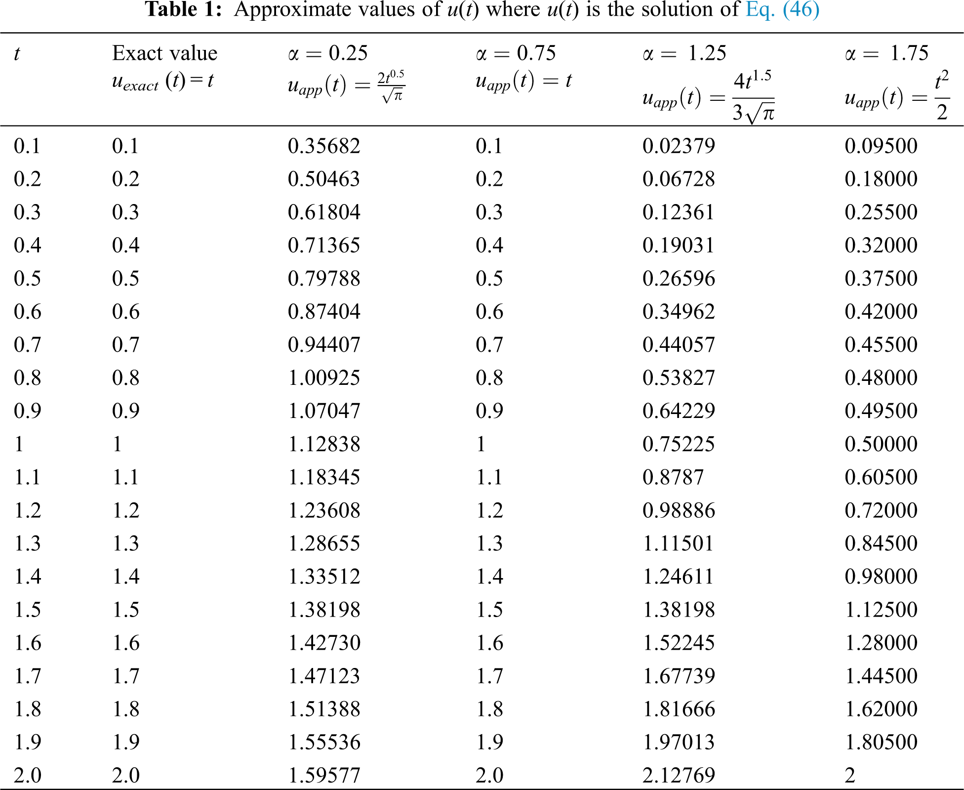
The estimate we will obtain in this section seems to be independent of interest. Without restriction of generality, we can assume α = 0.25,  0.75,  1.25 and α = 1.75 hold for t = 0.1,  0.2,  …, 2. We compute the experimentally determined solution of Eq. (46) for the different values of α with many values of t. This yields information about the analogue between the exact and approximate value of u(t).

Figs. 1–Figs. 4 show that there are intersections between exact uexact(t) = t and approximate value uapp(t)=2t0.5π,t,4t1.53π,t22 , respectively. Also, Tab. 1 contains all details.

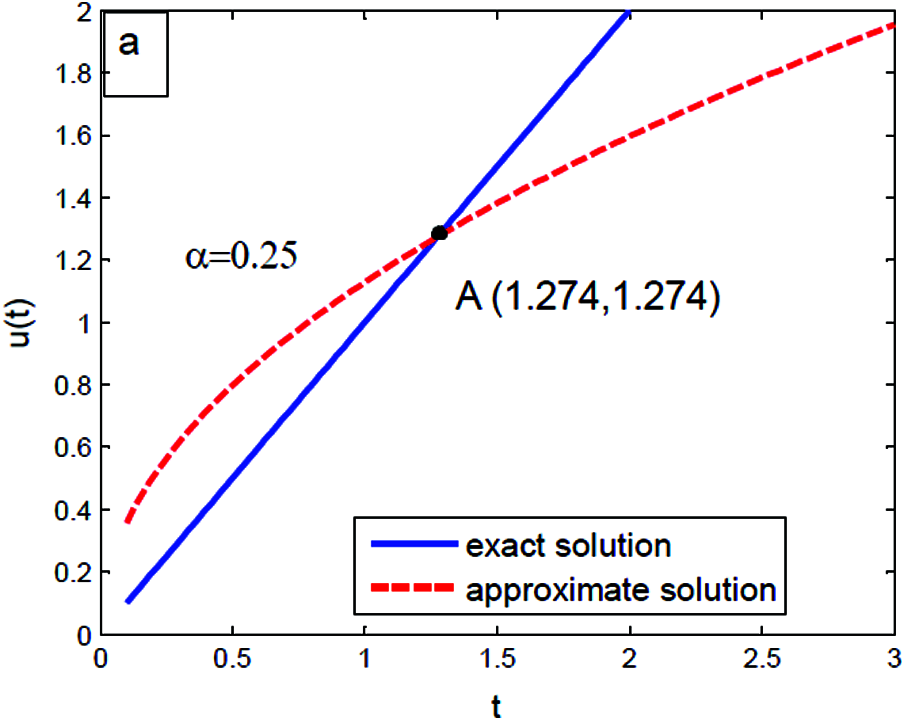
Figure 1: The experimentally determined solutions at t = 0.1, 0.2, …, 2 in Eq. (46) with α=0.25

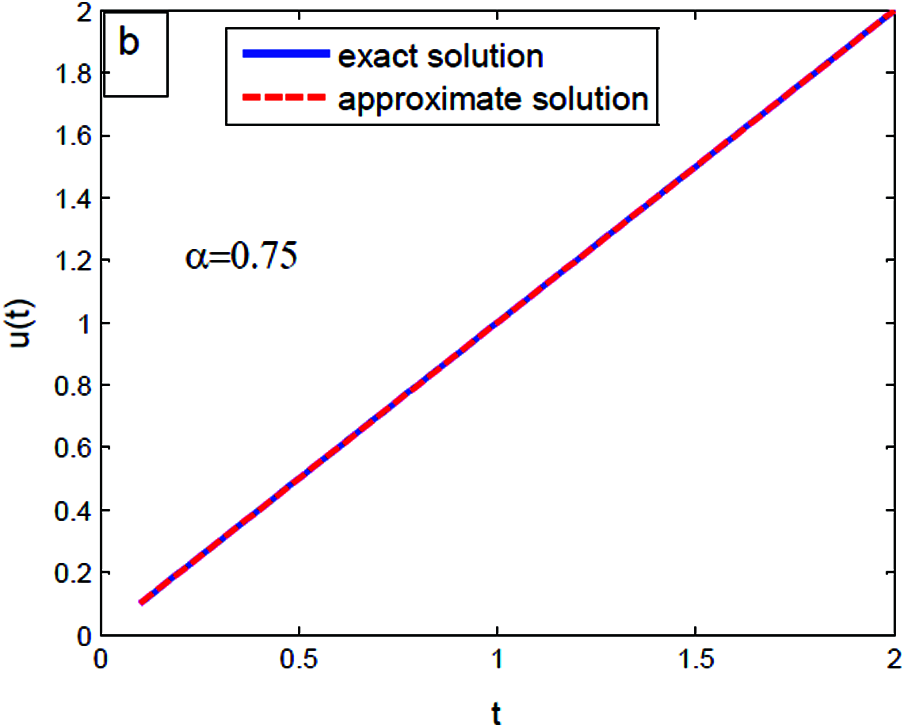
Figure 2: The experimentally determined solutions at t = 0.1, 0.2, …, 2 in Eq. (46) with α = 0.75

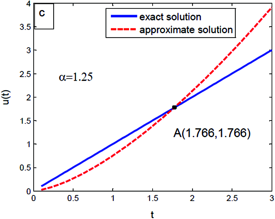
Figure 3: The experimentally determined solutions at t = 0.1, 0.2, …, 2 in Eq. (46) with α = 1.25

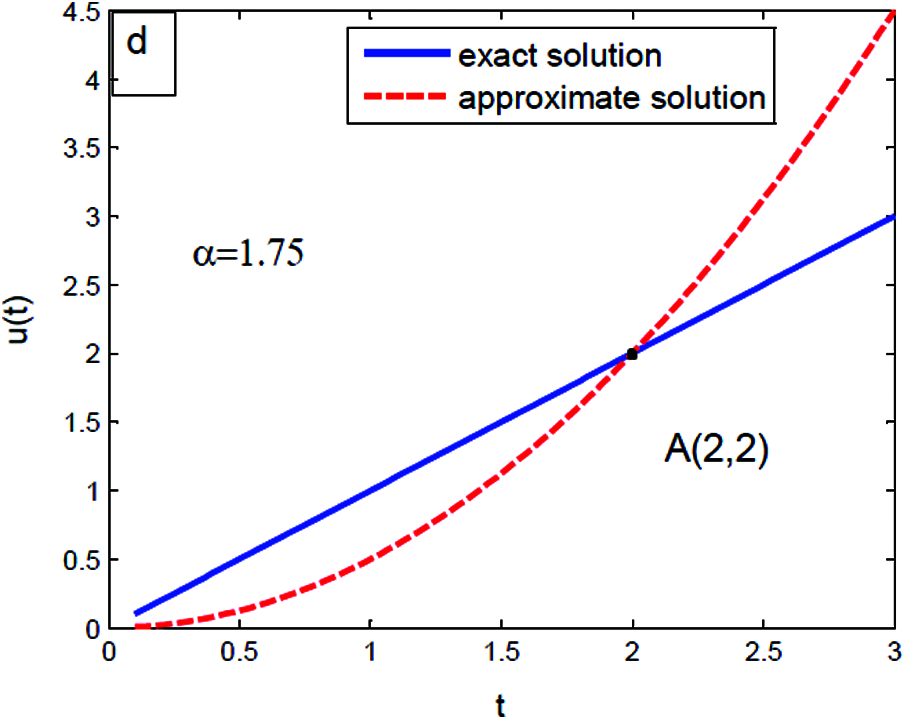
Figure 4: The experimentally determined solutions at t = 0.1, 0.2, …, 2 in Eq. (46) with α = 1.75

4  Special Cases

It is evident that this manuscript is more generalized from analogues papers. More remarkable special cases which are covered by a lot of last papers.

Remark 1 If the Eq. (7) has no delay item, it becomes fractional Volterra-Fredholm integro-differential equation [4].

Remark 2 If the Eq. (7) has no delay item and α = 1, it becomes integro-differential equation [2,14].

Remark 3 If the Eq. (7) has no delay item and it becomes Fractional integro-differential equation [11].

Remark 4 If the Eq. (7) has no delay item and no Volterra integral, it becomes fractional Fredholm integro-differential equation [8,11].

Remark 5 If the Eq. (7) has no delay item, no Volterra and no Fredholm integrals, it becomes fractional differential equation [5,9,11,16].

Remark 6 If the Eq. (7) has linear function of constant delay item, it becomes fractional Volterra-Fredholm integro-differential equation [15].

5  Conclusion

The benefit of modified several methods is that it successfully contributed to the rapidly progressing of the exact, approximate and numerical solutions. Also, modified methods are considered as a new powerful technique to solve a large range of equations such as differential, integral and integro-differential. At a certain value of α = 0.75 the approximate solution is equal to the exact solution. Also, the analogy between the exact and approximate solution differs from an example to others.

Acknowledgement: The authors are very grateful to the editors and reviewers for carefully reading the paper and for their comments and suggestions which have improved the paper.

Funding Statement: The authors received no specific funding for this study.

Conflicts of Interest: The authors declare that they have no conflicts of interest to report regarding the present study.

This work is licensed under a Creative Commons Attribution 4.0 International License, which permits unrestricted use, distribution, and reproduction in any medium, provided the original work is properly cited.