Sound & Vibration

DOI: 10.32604/sv.2022.011838

ARTICLE

A Suitable Active Control for Suppression the Vibrations of a Cantilever Beam

Y. A. Amer1, A. T. EL-Sayed2 and M. N. Abd EL-Salam3,*

1Mathematics Department, Science Faculty, Zagazig University, Zagazig, Egypt
2Basic Sciences Department, Modern Academy for Engineering and Technology, Cairo, Egypt
3Basic Sciences Department, Higher Technological Institute, 10th of Ramadan City, Egypt
*Corresponding Author: M. N. Abd EL-Salam. Email: mansour.naserallah@yahoo.com
Received: 31 May 2020; Accepted: 24 December 2021

1  Introduction

Many types of controllers are used for suppressing the vibrations of different non-linear dynamical systems such that, negative linear velocity feedback, negative cubic velocity feedback, non-linear saturation controllers (NSC), non-linear Integral Positive Position Feedback Controllers (NIPPF), the Integral resonant controllers (IRC) and time delay control. The technique of multiple time scales used to investigate the micro-beams non-linear vibrations for two different resonance cases (super-harmonic and harmonic resonances). From this investigation, there is a clear effect of the boundary conditions on the micro-beams vibrations [1]. Recently, the vibrations of many vibrating systems [2–7] has been studied. Because of the time delayed and active controls springiness [8–14] in controlling many vibrating system, many papers used time delay for suppressing the vibrations of non-linear systems. Abdelhafez et al. [15] investigated the effectiveness of time delays when the positive position controllers are used for suppressing the vibrations of a self-exited non-linear beam. They notified that, the time margin depends on the overall delays of the system τ1+τ2 . The authors in [16] investigated the influence of two different delays the first is displacement delay and the second is velocity delay in a cantilever beam. They used the method of multiple scales to determine all super-harmonic and sub-harmonic resonance cases.

Since the aim of most studies is to suppress the vibrations, one of the important types of control to vibrating systems is the PPF, which, described by a single degree of freedom system that, its frequency tuned to one of the structural frequencies. El-Ganaini et al. [17] presents the effectiveness of the PPF controller for decreasing the vibrations of nonlinear system at primary resonance and one-to-one internal resonance. They concluded that, PPF controller successful for systems that, has a small natural frequency. El-sayed et al. [18] achieved good results in decreasing the vibrations of vertical conveyor subject to external excitations by using PPF controllers such that, the vibrations in first mode reduced about 99.88% and the vibrations in the second mode reduced about 99.97% from its values without controllers. Ferrari et al. [19] offered an experimentally studying for the effectiveness of the PPF controllers on suspended the vibrations of sandwich plate. Niu et al. [20] realized the fractional-order positive position feedback (FOPPF) controller. They found that, the FOPPF controller gives better results comparing with PPF controller. Omidi et al. [21,22] presented three kinds of control to suppress the vibrations of vibrating systems such that, the Integral resonant controllers (IRC), PPF controllers and the non-linear Integral Positive Position feedback (NIPPF). The eminent type of decreasing the vibrations is NIPPF type. PPF controller and multimode modified positive position feedback (MMPPF) controllers are used for deceasing the vibrations of a flexible beam and a collocated structure, respectively [23,24].

In this article, four types of active vibrations controllers the linear velocity feedback control, the cubic velocity feedback control, NSC and PPF controller used to suppression the vibrations of a cantilever beam containing the cubic and fifth nonlinearity terms excited by an external force. The positive position feedback controller (PPF) is the suitable active control type for decreasing the cantilever beam’s vibrations. The approximate solution obtained applying the method of multiple scales up to first approximation. The stability of the cantilever beam investigated at the simultaneous resonance conditions (1:1 internal and primary). The behavior of the cantilever beam without and with PPF controller is simulated numerically. The influence of some chosen coefficient is illustrated numerically. The rapprochement between numeric and analytic solution is offered.

2  Mathematical Modelling

The equation of motion of a cantilever beam described by the following differential equation [15]:

x¨+α1x˙+β1x˙3+β2x˙5+ω12x+γ1x3+γ2x5+δ1(xx˙2+x2x¨)+δ2(x3x˙2+x4x¨)=fcos⁡(Ωt) (1)

where, x is the displacement of the cantilever beam. The damping coefficient represented by α1 . The nonlinearities terms coefficients are βj , γj and δj(j=1,2) . The excitation frequency and amplitude are Ω and f . For suppression the vibrations of the cantilever beam, we used four different types of controllers as the following.

The negative linear velocity feedback:

x¨+εα^1x˙+εβ^1x˙3+εβ^2x˙5+ω12x+εγ^1x3+εγ^2x5+εδ^1(xx˙2+x2x¨)+εδ^2(x3x˙2+x4x¨)=εf^cos⁡(Ωt)−εG^1 x˙ (2)

The negative cubic velocity feedback:

x¨+εα^1x˙+εβ^1x˙3+εβ^2x˙5+ω12x+εγ^1x3+εγ^2x5+εδ^1(xx˙2+x2x¨)+εδ^2(x3x˙2+x4x¨)=εf^cos⁡(Ωt)−εG^2 x˙3 (3)

The non-linear saturation controller:

x¨+εα^1x˙+εβ^1x˙3+εβ^2x˙5+ω12x+εγ^1x3+εγ^2x5+εδ^1(xx˙2+x2x¨)+εδ^2(x3x˙2+x4x¨)=εf^cos⁡(Ωt)+εη^1y2 (4a)

y¨+εα^2y˙+ω22y=εη^2xy (4b)

The positive position feedback controller:

x¨+εα^1x˙+εβ^1x˙3+εβ^2x˙5+ω12x+εγ^1x3+εγ^2x5+εδ^1(xx˙2+x2x¨)+εδ^2(x3x˙2+x4x¨)=εf^cos⁡(Ωt)+ελ^1y (5a)

y¨+εα^2y˙+ω22y=ελ^2x (5b)

where, ω1 and ω2 are the natural frequencies of the cantilever beam and the PPF controller. The control and feedback signals are λ^1 , η^1 , and λ^2 , η^2 . The feedback gains are G^1 and G^2 . To summarize the comparison between the four types of control, we explain the flowchart diagram as in Fig. 1.

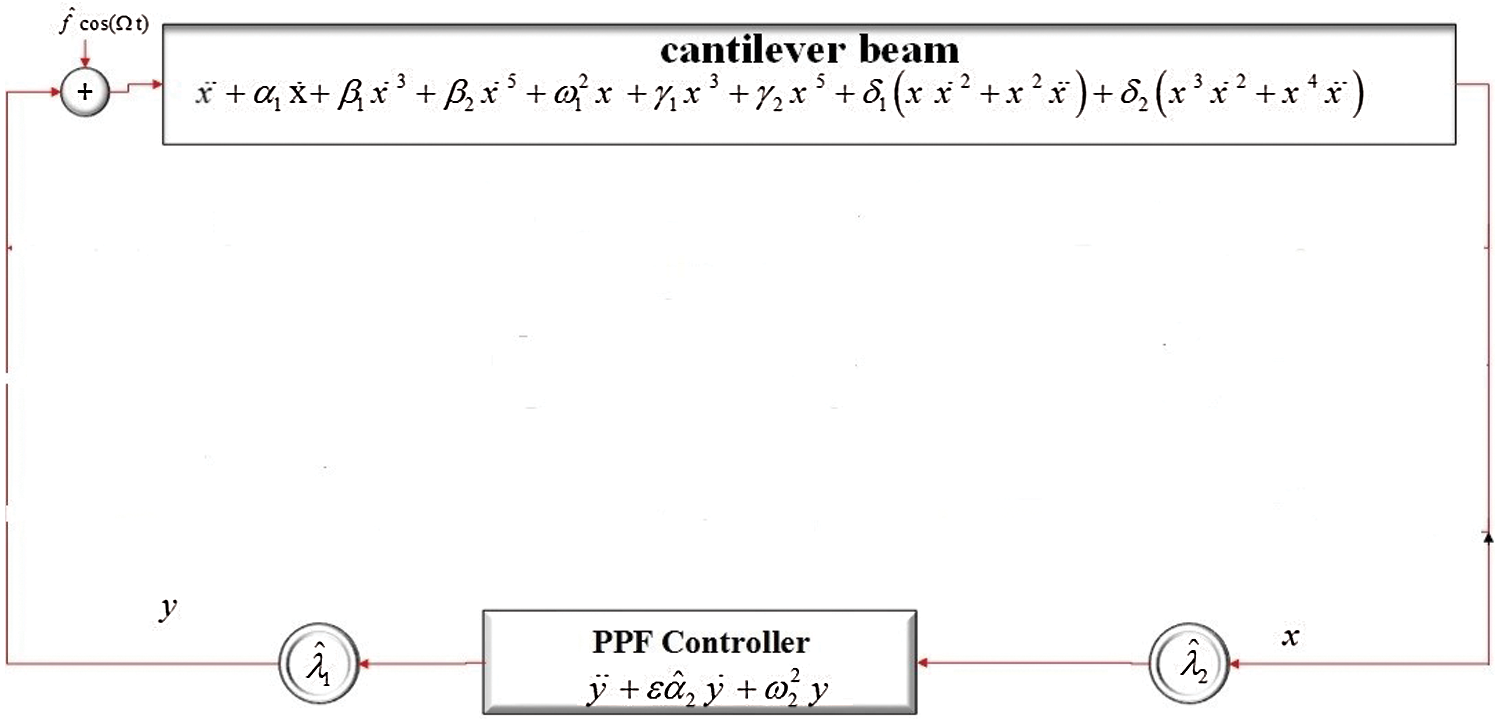
Figure 1: The flowchart diagram of the main system with PPF controller

2.1 Time History with Numerical Simulation

Numerically, the cantilever beam’s differential Eq. (1) was studied using Runge-Kutta 4th order method at the worst resonance case (One-to-one internal and primary resonance) at the following values of parameters:

ω 1 =1.4, β 1 =0.3331, β 2 =0.1299, γ 1 =0.3338, γ 2 =0.1319, δ 1 =3.2746, δ 2 =2.2, α 1 =0.005, f=0.01

At this study, we compare between four different types of controllers for suppressing the vibration of a cantilever beam. Fig. 2 presents the uncontrolled cantilever beam before using any type of controllers at the primary resonance case. In Fig. 3, we used two types of controllers to decrease the vibration of the system. The first type, is a negative cubic velocity feedback control which decreasing the vibration of the system to reach 0.13, so, the effectiveness of the control (Ea = amplitude of uncontrolled system/amplitude of controlled system) equal one as shown in Fig. 3a. The second type, is a negative linear velocity feedback control which decreasing the vibration of the system to reach 0.007, so, the effectiveness of the control Ea = 21 as shown in Fig. 3b. Fig. 4 illustrates the effectiveness of the non-linear saturation controller (NSC) on the cantilever beam. From this figure, we concluded that, the NSC controller minimized the vibration to reach 0.07 which means that Ea = 2. The positive position feedback controller (PPF) is the best type of controllers for suppressing the vibrations of the cantilever beam where it reduced the vibrations to 0.0006 and Ea = 250 as shown in Fig. 5. The solid lines elucidated the numerical solution of the main system before and after using the PPF controller while, dash lines elucidated the amplitude adjustments a1 and a2 for the generalized coordinates x and y . Finally, there is a good agreement between the numerical and analytical solutions of the main system and the PPF controller as presented in Figs. 2 and 5.

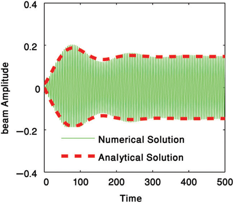
Figure 2: Uncontrolled system at primary resonance case

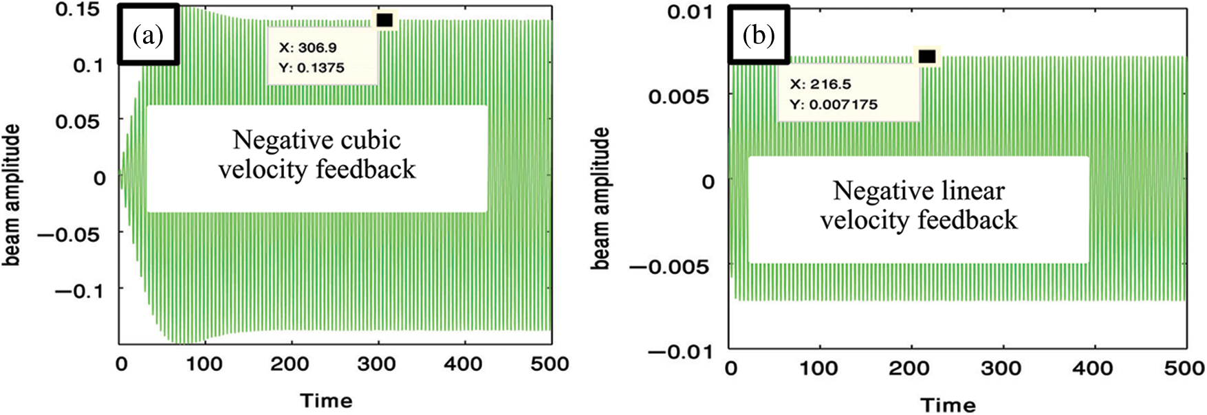
Figure 3: Negative cubic and linear velocity feedback for reducing the amplitude of the cantilever beam

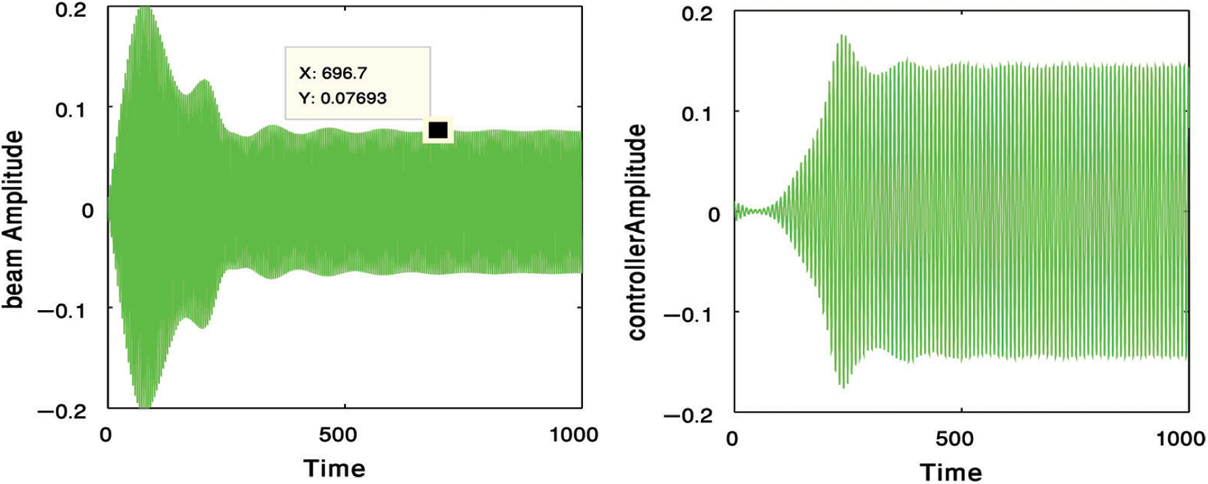
Figure 4: NSC controller for reducing the amplitude of the main system

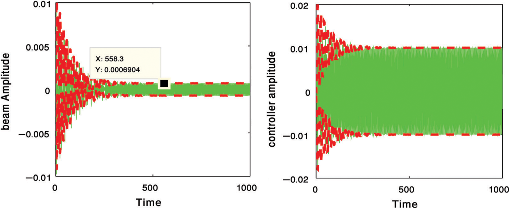
Figure 5: PPF controller for reducing the amplitude of the main system

2.2 Perturbation Analysis

According to the results that we obtained from Fig. 5, Which shows that the most appropriate controller is the PPF controller so we will study the main system after activating the PPF control. To get the approximate solution up to the first approximation, we applied the method of multiple scales [25,26] as the following:

x(t;ε)=x0(T0,T1)+εx1(T0,T1)+O(ε2)y(t;ε)=y0(T0,T1)+εy1(T0,T1)+O(ε2)} (6)

where, the fast scale is T0 and the slow scale is T1=εt . The derivatives using the multiple scales method take the forms:

ddt=D0+εD1+...d2dt2=D02+2εD0D1+...}Dj=∂∂Tj(j=0,1) (7)

Inserting Eqs. (4) and (5) in Eqs. (2) and (3) such that:

[D02+ω12]x0+ε[D02+ω12]x1=ε{f^cos⁡(Ωt)+λ^1y0−γ^1x03−γ^2x05−2D0D1x0−α^1D0x0−β^1(D0x0)3−β^2(D0x0)5−δ^1(x0(D0x0)2+x02D02x0)−δ^2(x03(D0x0)2+x04D02x0)}+O(ε2) (8)

[D02+ω22]y0+ε[D02+ω22]y1=ε[λ^2x0−2D0D1y0−α^2D0y0]+O(ε2) (9)

Equating the coefficients of the same power of ε :

O(ε0) :

[D02+ω12]x0=0 (10)

[D02+ω22]y0=0 (11)

O(ε) :

[D02+ω12]x1={f^cos⁡(Ωt)+λ^1y0−γ^1x03−γ^2x05−2D0D1x0−α^1D0x0−β^1(D0x0)3−β^2(D0x0)5−δ^1(x0(D0x0)2+x02D02x0)−δ^2(x03(D0x0)2+x04D02x0)} (12)

[D02+ω22]y1=[λ^2x0−2D0D1y0−α^2D0y0] (13)

Solving the homogenous differential Eqs. (10) and (11) to get the following:

x0(T0,T1)=A(T1)eiω1T0+A¯(T1)e−iω1T0 (14)

y0(T0,T1)=B(T1)eiω2T0+B¯(T1)e−iω2T0 (15)

Denote that A and B, are complex functions in T1 . For computation the right hand sides of Eqs. (12) and (13), we will replace x0 and y0 by its values in Eqs. (14) and (15) so that:

[D02+ω12]x1={[−2iω1D1A−iα^1ω1A−3iβ^1ω13A2A¯−10iβ^2ω15A3A¯2−3γ^1A2A¯+2δ^1ω12A2A¯−10γ^2A3A¯2+8δ^2ω12A3A¯2]eiω1T0+[iβ^1ω13A3+5iβ^2ω15A4A¯−γ^1A3−5γ^2A4A¯+2δ^1ω12A3+6δ^2ω12A4A¯]e3iω1T0+[−iβ^2ω15A5−γ^2A5+2δ^2ω12A5]e5iω1T0+[λ^1B]eiω2T0+[f^2]eiΩT0}+CC (16)

[D02+ω22]y1=[−2iω2D1B−iα^2ω2B]eiω2T0+[λ^2A]eiω1T0+CC (17)

The complex conjugate parts collected in the term CC. For getting the particular solutions of Eqs. (16) and (17), we will remove the secular terms such that:

x1(T0,T1)=H1(T1)e3iω1T0+H2(T1)e5iω1T0+H3(T1)eiω2T0+H4(T1)eiΩT0+CC (18)

y1(T0,T1)=H5(T1)eiω1T0+CC (19)

where Hj(j=1,...,5) offering complex functions in T1 which defined in the appendix. From the first approximation, we concluded the following resonance cases:

     i)  Primary resonance: Ω≅ω1

    ii)  Internal resonance: ω1≅ω2

   iii)  Simultaneous resonance: One-to-one internal and primary resonance.

3  Periodic Solutions

In this section, the selected one is simultaneous resonance ( Ω≅ω1 , ω1≅ω2 ) is used to discuss the solvability conditions, we will introduce two detuning parameters (σ1,σ2) so that:

Ω=ω1+εσ^1=ω1+σ1ω2=ω1+εσ^2=ω1+σ2} (20)

Including Eq. (20) into Eqs. (16) and (17) for compiling the solvability conditions as:

−2iω1D1A−iα^1ω1A−3iβ^1ω13A2A¯−10iβ^2ω15A3A¯2+(2δ^1ω12−3γ^1)A2A¯+(8δ^2ω12−10γ^2)A3A¯2+f^2eiσ^1T1+λ^1Beiσ^2T1=0 (21)

−2iω2D1B−iα^2ω2B+λ^2Ae−iσ^2T1=0 (22)

Exchanging A and B by the polar form as:

A(T1)=a1(T1)eiθ1(T1)B(T1)=a2(T1)eiθ2(T1)D1A(T1)=(a′1(T1)+ia1θ′1(T1))eiθ1(T1)D1B(T1)=(a′2(T1)+ia2θ′2(T1))eiθ2(T1)};()′=ddT1 (23)

where aj and θj(j=1,2) are the motion’s steady state phases and amplitudes. Subjoining Eq. (23) into Eqs. (21) and (22). For any two equal complex numbers, the real and imaginary parts are equal so that:

a1′=[−α^12]a1−[3β^1ω128]a13−[5β^2ω1416]a15+[f^2ω1]sin⁡ϕ1+[λ^12ω1]a2sin⁡ϕ2 (24)

a1θ1′=[3γ^18ω1−δ^1ω14]a13+[5γ^216ω1−δ^2ω14]a15−[f^2ω1]cosϕ1−[λ^12ω1]a2cos⁡ϕ2 (25)

a2′=[−α^22]a2−[λ^22ω2]a1sin⁡ϕ2 (26)

a2θ2′=−[λ^22ω2]a1cos⁡ϕ2 (27)

where, ϕ1=σ^1T1−θ1 and ϕ2=σ^2T1+θ2−θ1 . Back to the main system parameters, we have the following equations:

a˙1=[−α12]a1−[3β1ω128]a13−[5β2ω1416]a15+[f2ω1]sin⁡ϕ1+[λ12ω1]a2sin⁡ϕ2 (28)

a1θ˙1=[3γ18ω1−δ1ω14]a13+[5γ216ω1−δ2ω14]a15−[f2ω1]cosϕ1−[λ12ω1]a2cos⁡ϕ2 (29)

a˙2=[−α22]a2−[λ22ω2]a1sin⁡ϕ2 (30)

a2θ˙2=−[λ22ω2]a1cos⁡ϕ2 (31)

where, a1′=a˙1ε,a2′=a˙2ε,θ1′=θ˙1ε,θ2′=θ˙2ε and ()˙=ddt .

3.1 Fixed Point Solution

For steady-state solution, we maybe find the fixed point of the Eqs. (28)–(31) by putting a˙1=a˙2=0 and ϕ˙j=0(j=1,2) , so:

0=[−α12]a1−[3β1ω128]a13−[5β2ω1416]a15+[f2ω1]sin⁡ϕ1+[λ12ω1]a2sin⁡ϕ2 (32)

aσ1=[3γ18ω1−δ1ω14]a13+[5γ216ω1−δ2ω14]a15−[f2ω1]cosϕ1−[λ12ω1]a2cos⁡ϕ2 (33)

0=[−α22]a2−[λ22ω2]a1sin⁡ϕ2 (34)

a2(σ1−σ2)=−[λ22ω2]a1cos⁡ϕ2 (35)

From the preceding system, the trigonometric functions can be written as:

sin⁡ϕ1=[2ω1f]{[α12]a1+[3β1ω128]a13+[5β2ω1416]a15+[λ1ω2α22ω1λ2]a22a1} (36)

cosϕ1=[2ω1f]{[3γ18ω1−δ1ω14]a13+[5γ216ω1−δ2ω14]a15+[λ1(σ1−σ2)ω2λ2ω1]a22a1−σ1a1} (37)

sin⁡ϕ2=−[ω2α2λ2]a2a1 (38)

cos⁡ϕ2=−[2(σ1−σ2)ω2λ2]a2a1 (39)

Squaring then adding both sides of Eqs. (36) and (37) and Eqs. (38) and (39) to obtain the following two equations:

{[3γ18ω1−δ1ω14]a13+[5γ216ω1−δ2ω14]a15+[λ1(σ1−σ2)ω2λ2ω1]a22a1−σ1a1}2+{[α12]a1+[3β1ω128]a13+[5β2ω1416]a15+[λ1ω2α22ω1λ2]a22a1}2={f2ω1}2 (40)

ω22[4σ12+8σ1σ2+4σ22+α22]a22=[λ2a1]2 (41)

3.2 Equilibrium Solution of a Fixed Point

While in movement to evolve the steady state solution’s stability, start with the following procedures:

a1=a10+a11a2=a20+a21ϕ1=ϕ10+ϕ11ϕ2=ϕ20+ϕ21} (42)

where, a10 , a20 , ϕ10 and ϕ20 are the solutions of Eqs. (32)–(35). The perturbations a11 , a21 , ϕ11 and ϕ21 are very small comparing with a10 , a20 , ϕ10 and ϕ20 so, after substituting from Eq. (42) into Eqs. (28)–(31) we keep only the linear terms of a11 , a21 , ϕ11 and ϕ21 . From this procedure, we get the following system:

a˙11=r11a11+r12ϕ11+r13a21+r14ϕ21 (43)

ϕ˙11=r21a11+r22ϕ11+r23a21+r24ϕ21 (44)

a˙21=r31a11+r32ϕ11+r33a21+r34ϕ21 (45)

ϕ˙21=r41a11+r42ϕ11+r43a21+r44ϕ21 (46)

In the appendix, we defined the coefficients rij(i=1...4),(j=1...4) . The matrix form of the previous system can be written as:

[a˙11ϕ˙11a˙21ϕ˙21]T=[D][a11ϕ11a21ϕ21]T (47)

where [D] is the Jacobian of the previous Eqs. (43)–(46). The Eigen-values of [D] determined from extract the following determinant:

|λ−r11r12r13r14r21λ−r22r23r24r31r32λ−r33r34r41r42r43λ−r44|=0 (48)

which, are the roots of the following polynomial:

λ4+Γ1λ3+Γ2λ2+Γ3λ+Γ4=0 (49)

where Γi;(i=1,...,4) are the coefficients of Eq. (49) that, defined in the appendix. For the above system’s solution to be stable, the Routh-Hurwitz criterion must be satisfied such that:

Γ1>0,Γ1Γ2−Γ3>0,Γ3(Γ1Γ2−Γ3)−Γ12Γ4>0,Γ4>0 (50)

4  Numerical Investigation

Eqs. (40) and (41) solved numerically to obtain the graphical solution for the amplitudes of both cantilever beam and the PPF controller via the detuning parameter (σ1) which, represented by two peaks. Fig. 6 presents the frequency response curves of the cantilever beam and the PPF controller where, the stable solution represented by the solid line and the dash one using for the unstable solution. From this figure, we concluded that the minimum value of the cantilever beam amplitude occurs at σ1=0 which means that, the PPF controller is capable of suppress the vibrations of the cantilever beam at the primary resonance case. For increasing values of a harmonic excitation force, the amplitudes of both the main system and the PPF controller increase, the jump phenomena occurs and the minimum value of the cantilever beam amplitude occurs at σ1=0 as illustrates in Figs. 7a and 7b.

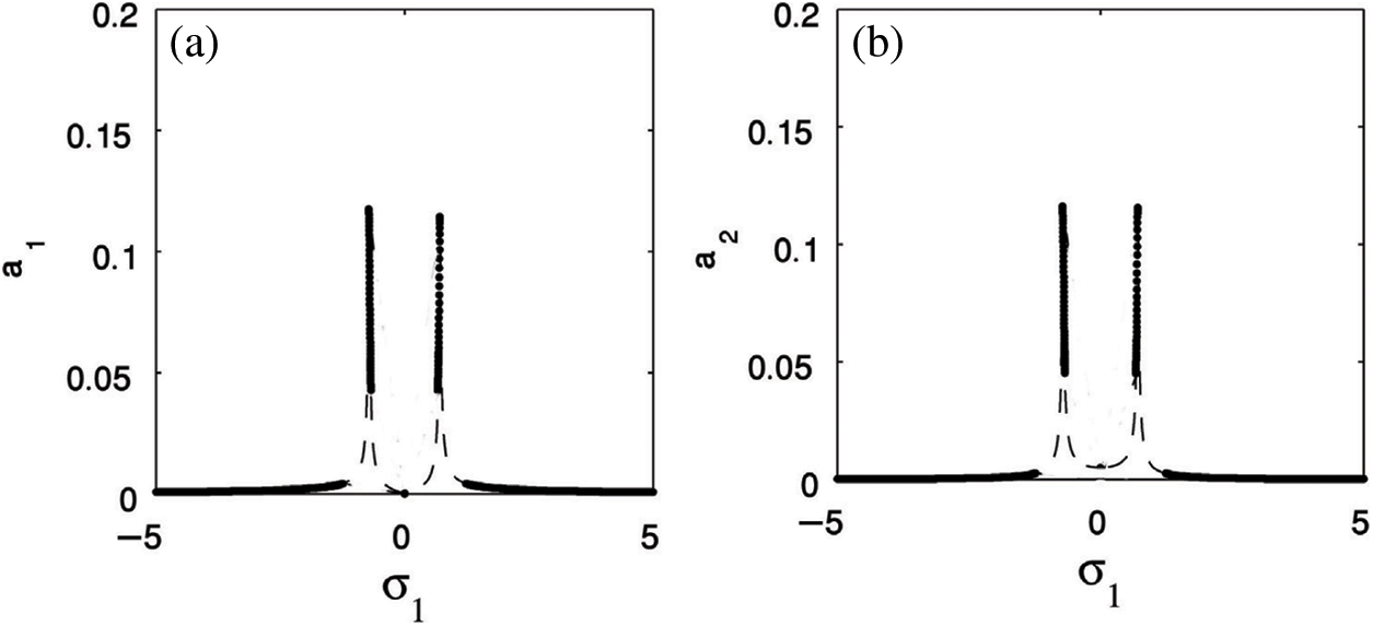
Figure 6: The response curves (a) The cantilever beam (b) The PPF controller

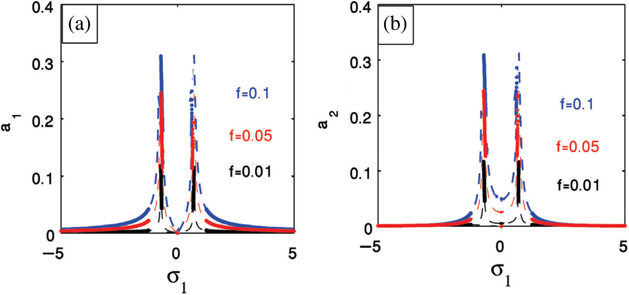
Figure 7: External force efficacy on (a) The cantilever beam (b) The PPF controller

For small values of natural frequency for σ2=0 , i.e., ( ω1=ω2 ), the cantilever peak amplitude and the PPF controller peak amplitude increases and the bandwidth of the vibration reduction increases so, in the case of small natural frequency the PPF controller is very acceptable as shown in Fig. 8. The bandwidth of the vibration reduction of the main system increases by increasing the values of the control signal λ1 and the feedback signal λ2 as represented in Figs. 9a and 10a. Fig. 9b shows that the PPF controller amplitude is monotonic decreasing function of the control signal λ1 . Fig. 10b shows that the PPF controller amplitude is monotonic increasing function of the feedback signal λ2 . For three different values of the internal detuning parameter σ2 , Fig. 11 shows the frequency response curves of both the cantilever beam and PPF controller. From this figure, the minimum of the steady state amplitudes of both the cantilever beam and PPF controller happens when σ1=σ2 . From Fig. 12, there is a good agreement between the frequency response curves (FRC) which given by the solid line and the numerical solution of Eq. (1) using (RK-4) that marked by green circles.

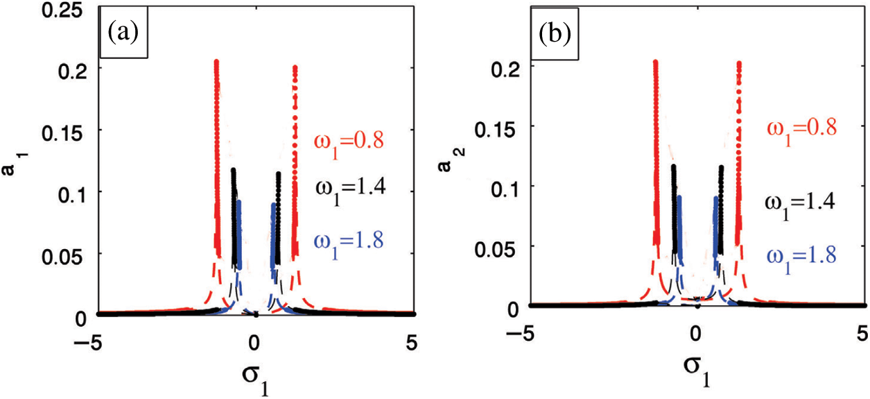
Figure 8: Natural frequency efficacy on (a) The cantilever beam (b) The PPF controller

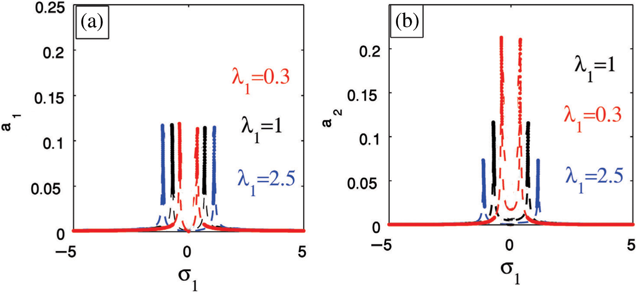
Figure 9: Control signal λ1 efficacy on (a) The cantilever beam (b) The PPF controller

Figure 10: Feedback signal λ2 efficacy on (a) The cantilever beam (b) The PPF controller

Figure 11: Detuning parameter σ2 efficacy on (a) The cantilever beam (b) The PPF controller

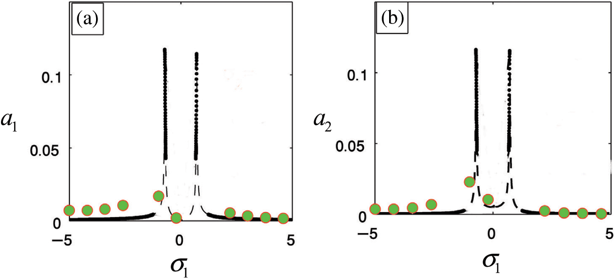
Figure 12: Comparison between the FRC solution and RK-4 solution

4.1 Influence of the Nonlinear Parameters

In the presence of the PPF controller, we studied the effectiveness of increases of all nonlinear parameters on the main system. The amplitude of the main system change either in decreasing or in increasing but this effect is very small so it do not appear clearly. For the nonlinear parameters β1 , γ1 and δ1 , the range of the amplitude of the main system from 0.00070069 to 0.00070087 as observed on Figs. 13a, 13c and 13e. For the nonlinear parameters β2 , γ2 and δ2 , the range of the amplitude of the main system from 0.00070071734 to 0.00070071736 as observed on Figs. 13b, 13d and 13f.

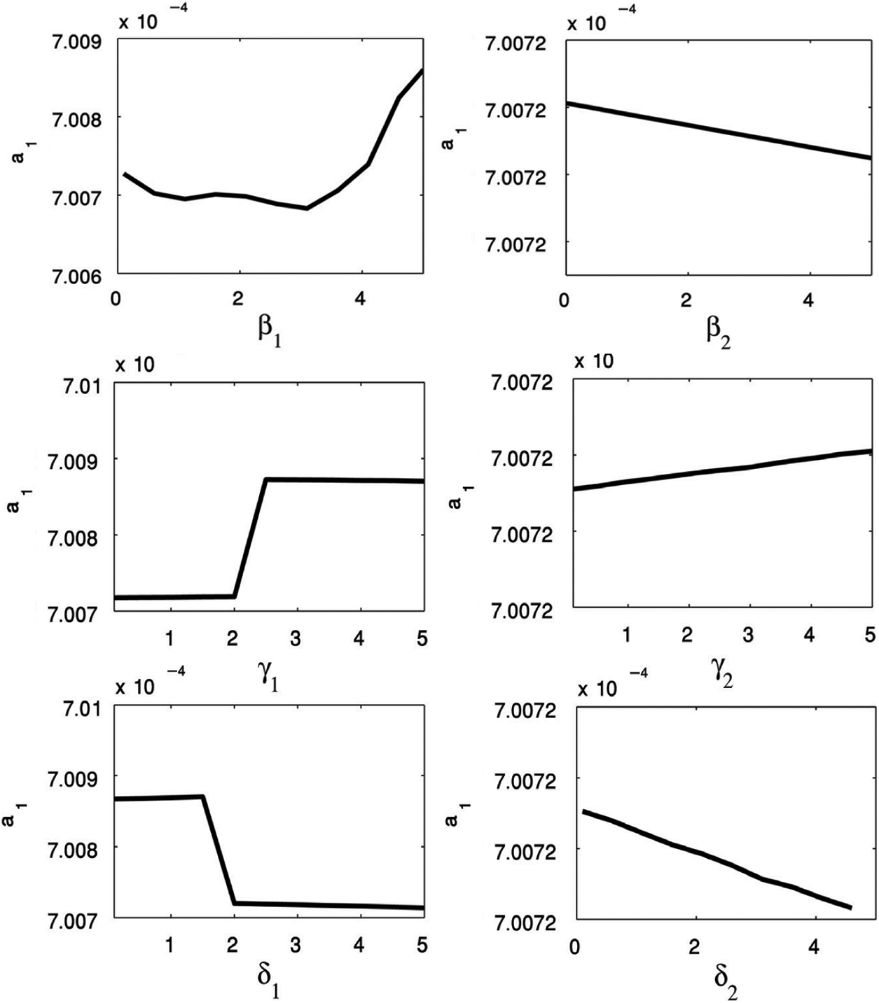
Figure 13: The influence of the nonlinear parameters on the main system amplitude

5  Conclusion

In this paper, we used four different types of active controllers for suppression the vibrations of the cantilever beam excited by an external force. Those four types are the linear velocity feedback control, the cubic velocity feedback control, the non-linear saturation controller (NSC) and the positive position feedback (PPF) controller. The best active control type for suppression the vibrations of the cantilever beam at the primary resonance case is the positive position feedback controller PPF as the following reasons:

     i)  Its effectiveness Ea equal 250 which more than the effectiveness of any type of controllers used to control the vibrating cantilever beam in this study.

    ii)  It is a suitable for small natural frequencies as the bandwidth of the vibration reduction increases.

Farther more, the steady state amplitude is monotonic increasing function on the external excitation force. The bandwidth of the vibration reduction increases for increasing values of the control signal λ1 and the feedback signal λ2 . Finally, there is a good agreement between the frequency response curves (FRC) and the numerical solution using (RK-4). The nonlinear parameters have a very small effect either in decreasing or in increasing the main system amplitude.

Funding Statement: The authors received no specific funding for this study.

Conflicts of Interest: The authors declare that they have no conflicts of interest to report regarding the present study.

References

 1.  Onur Ekici, H., Boyaci, H. (2007). Effects of non-ideal boundary conditions on vibrations of microbeams. Journal of Vibration and Control, 13, 1369–1378. DOI 10.1177/1077546307077453. [Google Scholar] [CrossRef]

 2.  Kuang, J. H., Chen, C. J. (2004). Dynamic characteristics of shaped micro-actuators solved using the differential quadrature method. Journal of Micromechanics and Microengineering, 14, 647–655. DOI 10.1088/0960-1317/14/4/028. [Google Scholar] [CrossRef]

 3.  Abdel-Rahman, E. M., Younis, M. I., Nayfeh, A. H. (2002). Characterization of the mechanical behavior of an electrically actuated microbeam. Journal of Micromechanics and Microengineering, 12(6), 759–766. DOI 10.1088/0960-1317/12/6/306. [Google Scholar] [CrossRef]

 4.  Younis, M. I., Nayfeh, A. H. (2003). A study of the nonlinear response of a resonant microbeam to an electric actuation. Nonlinear Dynamics, 31(1), 91–117. DOI 10.1023/A:1022103118330. [Google Scholar] [CrossRef]

 5.  Amer, Y. A., EL-Sayed, A. T., EL-Salam, M. A. (2018). Non-linear saturation controller to reduce the vibrations of vertical conveyor subjected to external excitation. Asian Research Journal of Mathematics, 11(2), 1–26. DOI 10.9734/ARJOM/2018/44590. [Google Scholar] [CrossRef]

 6.  Eftekhari, M., Ziaei-Rad, S., Mahzoon, M. (2013). Vibration suppression of a symmetrically cantilever composite beam using internal resonance under chordwise base excitation. International Journal of Non-Linear Mechanics, 48, 86–100. DOI 10.1016/j.ijnonlinmec.2012.06.011. [Google Scholar] [CrossRef]

 7.  Nayfeh, A. H., Younis, M. I. (2005). Dynamics of MEMS resonators under superharmonic and subharmonic excitations. Journal of Micromechanics and Microengineering, 15(10), 1840–1847. DOI 10.1088/0960-1317/15/10/008. [Google Scholar] [CrossRef]

 8.  Amer, Y. A., El-Sayed, A. T., El-Bahrawy, F. T. (2015). Torsional vibration reduction for rolling mill’s main drive system via negative velocity feedback under parametric excitation. Journal of Mechanical Science and Technology, 29(4), 1581–1589. DOI 10.1007/s12206-015-0330-8. [Google Scholar] [CrossRef]

 9.  Amer, Y. A., El-Sayed, A. T., Kotb, A. A. (2016). Nonlinear vibration and of the Duffing oscillator to parametric excitation with time delay feedback. Nonlinear Dynamics, 85(4), 2497–2505. DOI 10.1007/s11071-016-2840-z. [Google Scholar] [CrossRef]

10. Yaman, M. (2009). Direct and parametric excitation of a nonlinear cantilever beam of varying orientation with time-delay state feedback. Journal of Sound and Vibration, 324(3–5), 892–902. DOI 10.1016/j.jsv.2009.02.010. [Google Scholar] [CrossRef]

11. Alhazza, K. A., Majeed, M. A. (2012). Free vibrations control of a cantilever beam using combined time delay feedback. Journal of Vibration and Control, 18(5), 609–621. DOI 10.1177/1077546311405700. [Google Scholar] [CrossRef]

12. Cai, G. P., Yang, S. X. (2006). A discrete optimal control method for a flexible cantilever beam with time delay. Journal of Vibration and Control, 12(5), 509–526. DOI 10.1177/1077546306064268. [Google Scholar] [CrossRef]

13. Mirafzal, S. H., Khorasani, A. M., Ghasemi, A. H. (2016). Optimizing time delay feedback for active vibration control of a cantilever beam using a genetic algorithm. Journal of Vibration and Control, 22(19), 4047–4061. DOI 10.1177/1077546315569863. [Google Scholar] [CrossRef]

14. Amer, Y. A., El-Sayed, A. T., Abd El-Salam, M. N. (2020). Position and velocity time delay for suppression vibrations of a hybrid Rayleigh-Van der Pol-Duffing oscillator. Sound & Vibration, 54(3), 149–161. DOI 10.32604/sv.2020.08469. [Google Scholar] [CrossRef]

15. Abdelhafez, H., Nassar, M. (2016). Effects of time delay on an active vibration control of a forced and self-excited nonlinear beam. Nonlinear Dynamics, 86(1), 137–151. DOI 10.1007/s11071-016-2877-z. [Google Scholar] [CrossRef]

16. Liu, C. X., Yan, Y., Wang, W. Q. (2019). Primary and secondary resonance analyses of a cantilever beam carrying an intermediate lumped mass with time-delay feedback. Nonlinear Dynamics, 97(2), 1175–1195. DOI 10.1007/s11071-019-05039-w. [Google Scholar] [CrossRef]

17. El-Ganaini, W. A., Saeed, N. A., Eissa, M. (2013). Positive position feedback (PPF) controller for suppression of nonlinear system vibration. Nonlinear Dynamics, 72(3), 517–537. DOI 10.1007/s11071-012-0731-5. [Google Scholar] [CrossRef]

18. El-Sayed, A. T., Bauomy, H. S. (2016). Nonlinear analysis of vertical conveyor with positive position feedback (PPF) controllers. Nonlinear Dynamics, 83(1–2), 919–939. DOI 10.1007/s11071-015-2377-6. [Google Scholar] [CrossRef]

19. Ferrari, G., Amabili, M. (2015). Active vibration control of a sandwich plate by non-collocated positive position feedback. Journal of Sound and Vibration, 342, 44–56. DOI 10.1016/j.jsv.2014.12.019. [Google Scholar] [CrossRef]

20. Niu, W., Li, B., Xin, T., Wang, W. (2018). Vibration active control of structure with parameter perturbation using fractional order positive position feedback controller. Journal of Sound and Vibration, 430, 101–114. DOI 10.1016/j.jsv.2018.05.038. [Google Scholar] [CrossRef]

21. Omidi, E., Mahmoodi, S. N. (2015). Sensitivity analysis of the nonlinear integral positive position feedback and integral resonant controllers on vibration suppression of nonlinear oscillatory systems. Communications in Nonlinear Science and Numerical Simulation, 22(1–3), 149–166. DOI 10.1016/j.cnsns.2014.10.011. [Google Scholar] [CrossRef]

22. EL-Sayed, A. T., Bauomy, H. S. (2018). Outcome of special vibration controller techniques linked to a cracked beam. Applied Mathematical Modelling, 63, 266–287. DOI 10.1016/j.apm.2018.06.045. [Google Scholar] [CrossRef]

23. Jun, L. (2010). Positive position feedback control for high-amplitude vibration of a flexible beam to a principal resonance excitation. Shock and Vibration, 17(2), 187–203. DOI 10.1155/2010/286736. [Google Scholar] [CrossRef]

24. Omidi, E., Mahmoodi, S. N. (2015). Multimode modified positive position feedback to control a collocated structure. Journal of Dynamic Systems, Measurement, and Control, 137(5), 1–7. DOI 10.1115/1.4029030. [Google Scholar] [CrossRef]

25. Nayfeh, A. H., Mook, D. T. (1979). Nonlinear oscillations. New York: Wiley. [Google Scholar]

26. Marinca, V., Herisanu, N. (2012). Nonlinear dynamical systems in engineering: Some approximate approaches. USA: Springer Science & Business Media. [Google Scholar]

Appendix

H1(T1)=iβ^1ω13A3+5iβ^2ω15A4A¯−γ^1A3−5γ^2A4A¯+2δ^1ω12A3+6δ^2ω12A4A¯−8ω12 ,

H2(T1)=−iβ^2ω15A5−γ^2A5+2δ^2ω12A5−24ω12 , H3(T1)=λ^1Bω12−ω22 , H4(T1)=f^2(ω12−Ω2) and H5(T1)=λ^2Aω22−ω12 , r11=−[α12+9β1ω128a102+25β2ω1416a104] , r12=[f2ω1cos⁡(ϕ10)] ,

r13=[λ12ω1sin(ϕ20)] , r14=[λ12ω1a20cos(ϕ20)] ,

r21=[σ1a10+3δ1ω14a10−9γ18ω1a10−25γ216ω1a103+5δ2ω14a103] ,

r22=−[f2ω1a10sin⁡(ϕ10)] , r23=[λ12ω1a10cos⁡(ϕ20)] , r24=−[λ12ω1a10a20sin(ϕ20)] ,

r31=−[λ22ω2sin⁡(ϕ20)]

r32=0 , r33=−[α22] , r34=−[λ22ω2a10cos(ϕ20)] ,

r41=[σ1a10+3δ1ω14a10−9γ18ω1a10−25γ216ω1a103+5δ2ω14a103−λ22ω2a20cos⁡(ϕ20)] ,