| Sound & Vibration |
DOI: 10.32604/sv.2022.014910
ARTICLE
Application of Machine Learning for Tool Condition Monitoring in Turning
1School of Mechanical and Building Sciences, VIT University, Chennai, Tamil Nadu, 600127, India
2Department of Mechanical Engineering, College of Engineering, Pune, 411005, India
*Corresponding Author: R. Jegadeeshwaran. Email: krjegadeeshwaran@gmail.com
Received: 07 November 2020; Accepted: 26 May 2021
Abstract: The machining process is primarily used to remove material using cutting tools. Any variation in tool state affects the quality of a finished job and causes disturbances. So, a tool monitoring scheme (TMS) for categorization and supervision of failures has become the utmost priority. To respond, traditional TMS followed by the machine learning (ML) analysis is advocated in this paper. Classification in ML is supervised based learning method wherein the ML algorithm learn from the training data input fed to it and then employ this model to categorize the new datasets for precise prediction of a class and observation. In the current study, investigation on the single point cutting tool is carried out while turning a stainless steel (SS) workpeice on the manual lathe trainer. The vibrations developed during this activity are examined for failure-free and various failure states of a tool. The statistical modeling is then incorporated to trace vital signs from vibration signals. The multiple-binary-rule-based model for categorization is designed using the decision tree. Lastly, various tree-based algorithms are used for the categorization of tool conditions. The Random Forest offered the highest classification accuracy, i.e., 92.6%.
Keywords: Machine learning; statistical analysis; tree based classification; turning
In turning operation, the single point cutting tool (SPCT) is employed to eliminate unwanted material from cylindrical bars. A machine tool used is called lathe on which surfaces of revolution can also be produced, i.e., a cylinder, a cone, a flat surface, grooves, threads, frustums of cones, etc. The cylindrical bar (work) is being held on a holding device called a ‘chuck’ and ‘tool post’ is a location of a cutting tool. So, hold the two securely and provide relative motion this is the main function of the machine tool [1,2]. Improper amount of movement, selection of speed of machining, feed of tool, and the cut depth result in breakage of the tool. Catastrophic failure might be occurring due to breakage say in the very beginning itself the tool is not very strong and one does not estimate it and suddenly it breaks off. It has to be avoided at all costs. Cutting may edge itself individual might be dulling of very fast without any this effect manifesting itself before that itself, those things are not considered when dealing with the gradual phenomenon of wear this takes place very gradually. This is because the tool deteriorates quality when it is being put to use where the chip is rubbing against the rake surface while moving and also applying a considerable amount of force very frequently in the order of hundreds of neutrons [3–5]. A Tool Condition Monitoring (TCM) is a predictive maintenance system used for mechanical systems or machine tools that monitor the condition of a cutting tool. Due to continuous usage of cutting tool, tool supervision is essential for improvement of manufacturing industry. TCM comprises hardware and software parts to achieve collecting & processing of signal, extraction & selection of features and lastly making a decision. Direct measurement gives precise information about the physical wear of the machining tool. In indirect measurement, different signal acquired, namely vibration, acoustic emission, cutting force, temperature, spindle current, and signal processing carried out. This method is easy to install and simple for real-time online installation. Hence indirect measurement is more suitable for tool condition monitoring [6]. Tool wear means that whenever a tool is being used for removing material, after a few minutes if the tip of the tool is observed which is defined by the intersections of the principal flank, auxiliary flank, and rake surface, it can be noticed that it has undergone a change. Generally, a study related to flank wear growth is considered to be interesting. Flank wear growth has a limit after which one does not use these turning tools. Flank wear, in the beginning, it grows when wear is setting in there are lots of ups and downs on the surface. The surface in the microstructural level will show lots of ups and downs these will engage with the workpiece, asperities, and rapid break take place when it has broken off or maybe flattened or abraded, etc., phenomena take place and this is rapid braking wear. The failure of tool is indicated in many ways. The surface finish which is obtained on the workpiece it is not acceptable, it is deteriorating; there might be vibration and chatter. There can be an increase in power consumption etc. There can be increase in the sound, there can be too much heat coming out from the color of the chips etcetera. So, lots of indicators will be there showing that the tool has become they reach a particular amount of wear [7–9]. As compared to other major industries of a country, the manufacturing industry plays a very crucial role in building the national economy. Processes like grinding, milling, etc., hence become an important consideration [10]. As this a profit-based industry, a lot of emphases is given on increasing the efficiency of the processes while maintaining the quality of products [11]. To achieve this, manufacturers tend to resort to high cutting speeds to save time. This leads to stress concentration on the tool and a rise in its temperature which hampers the product quality as well as the tool condition [12]. Problems like this alarmed the need for tool condition monitoring. For the past 2 decades, TCM has been a matter of contention in industrial as well as academic research [13]. Hence, today, we have various methods of monitoring a tool comprising of analytical as well as computational. Leo [14] designed a time-domain analytical model for TCM but its use was restricted by the complexity of involved mathematics for different machines. Analysis using acoustic emissions gained popularity in the last decade after Li [15] used it for TCM. Another method used for the purpose of monitoring was ultrasonic analysis [16]. After recent developments in ML and considering the availability of various tools, a new, more efficient method was found and has been in use ever since, i.e., use of machine learning techniques for TCM. Many different algorithms are in use for the purpose. K-star algorithm is a unique one and was successfully implemented for monitoring [17]. Another method used by Elangovan et al. [18] stated that using Bayes classifiers, that statistical features provide more information about a tool than the histogram. Several TCM methods have emerged over time, for e.g., in the milling process, acoustic emission, sensor fusion technique, thermal imaging, Machine Learning, etc. [19]. Recently, the application of ML algorithms in creating a flank wear prediction model, during the milling process has proved to be promising [20,21]. The review conveys that tool failure is undesirable because it affects the accuracy and economics of machining. So, tool monitoring scheme (TMS) for categorization and prediction of failures has become the utmost priority. In an era of machine learning, training and classifying data has turn out to be fast, reliable and worthy. Hence the incorporation of these modern approaches with traditional TMS is really a need of an hour. The machine learning scheme really has a potential and can be implemented in real-time fault classification. In the current study, investigation on the single point cutting tool is carried out while turning a stainless steel (SS) workpeice on the manual lathe trainer. The vibrations developed during this activity are examined for failure-free and various failure states of a tool. The statistical modeling is then incorporated to trace vital signs from vibration signals. The multiple-binary-rule-based model for categorization is designed using the decision tree. Lastly, various tree-based algorithms are used for the categorization of tool conditions. The framework is presented in Fig. 1.
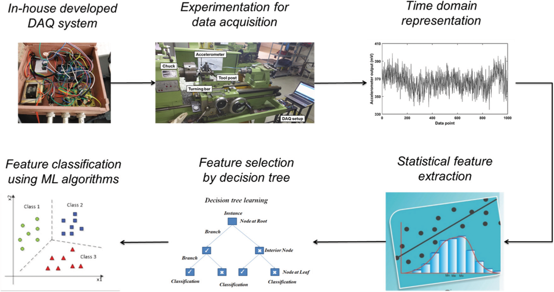
Figure 1: Framework of the research
The experimental arrangement and procedure used for the turning and vibration collection are stated here. Fig. 2 represents the experimental arrangement with various components. It is comprised of a conventional lathe machine (Make: Samrat Machine Tools Lathe SMTA808), a micro-electro-mechanical (MEM) accelerometer, and a data logger. The data logger is developed using a microcontroller Arduino ATmega2560 and a computer for acquiring, conditioning, processing and storing the data from the accelerometer [22,23]. The data was communicated from Arduino software to MS-Excel using software called Parallax-DAQ. The cylindrical bar of Stainless Steel with dia. 70 mm was positioned in a rotating chuck (work holding) and a cutting tool was secured on the tool post. It is a well-known fact that the vibration progressed during milling will be conveyed on either side of tool and workpiece. But with the intention to find tool faults, the accelerometer has to be placed on the tool post to serve the cause. Hence, the MEMS accelerometer (Analogue ADXL335) of sensitivity 330 mv/g was directly connected to a tool post using a sticky material. A relationship exists between the tool’s rigidity and the vibrations produced during turning operation. The cataclysmic frequencies of over 500 Hz are produced during the turning process. It also proved the impact of the work piece’s rigidity and its surface roughness on vibration signals. Hence, in the turning process, vibration signals prove to be a vital parameter for fault classification. The input machining parameters were selected as follows: vertical cut depth: 0.02 cm, machining speed: 8800 cm/min & the feed per revolution: 0.01 mm. This selection was done w.r.t. the standard catalogue and usual calculations as discussed below. A best combination of speed, feed, and depth is needed for a CNC operation, which are the typical parameters selected for the same. This combination depends on the type of operation being performed, workpiece material, etc., with reference to the standard catalogue.
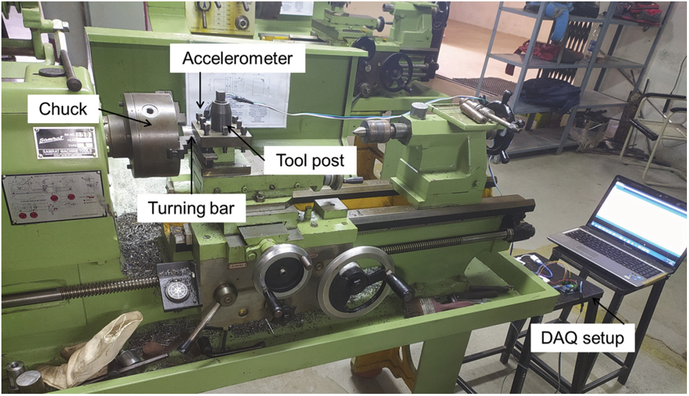
Figure 2: Experimental arrangement
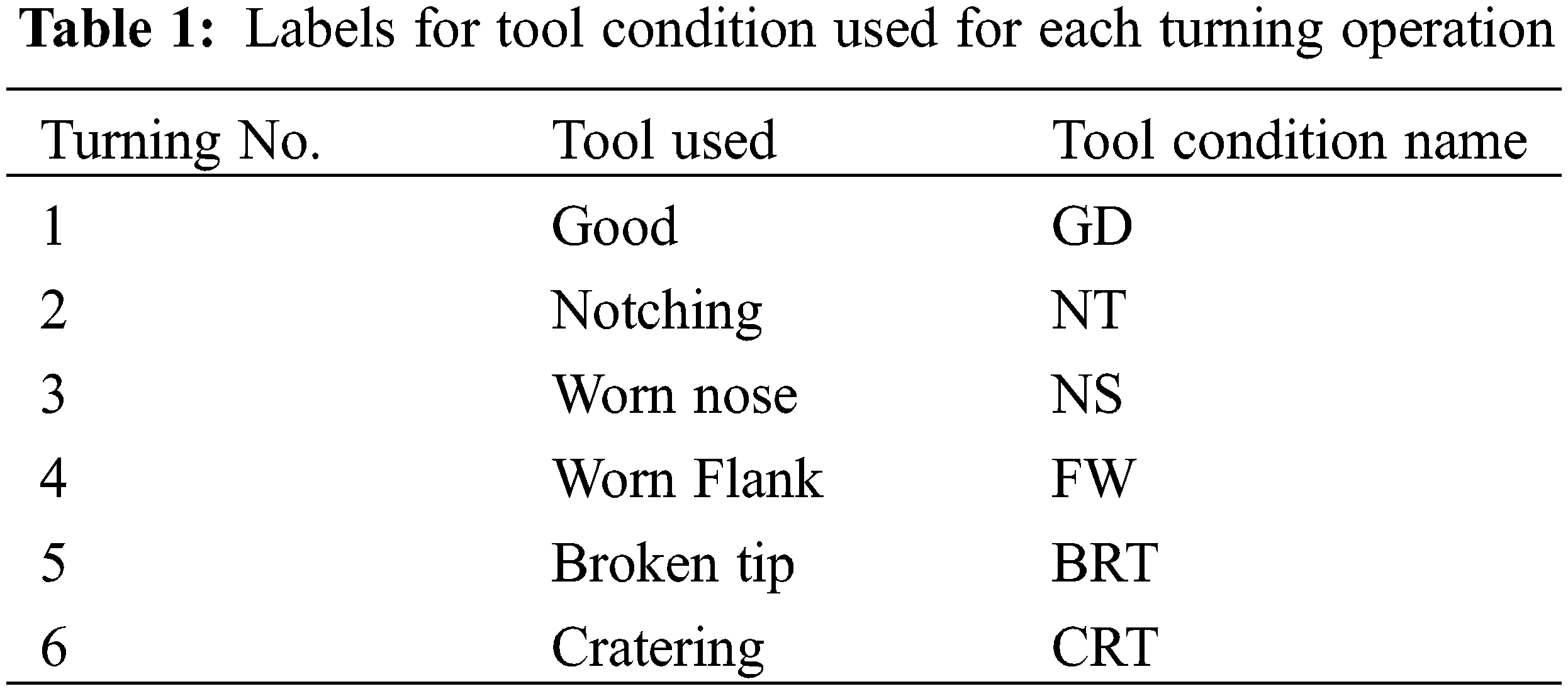
The turning was performed using a healthy tool first and then using faulty tools. The tool with previously built-in faults such as broken tip, notching, worn flank, worn nose and cratering were considered. The labels for the tool condition category are stated in Table 1.
The machining speed can be determined by
Here,
Putting this in Eq. (1), we obtain, machining speed =
A feed per revolution can be determined by
where
Putting this in Eq. (2), we obtain, feed = F = 0.01 cm/rev.
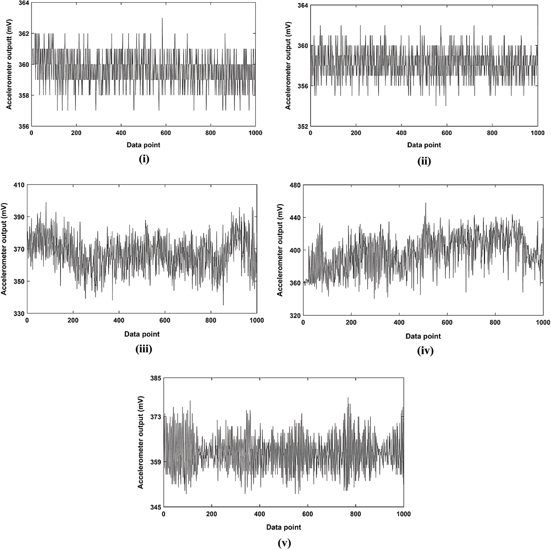
Figure 3: (i) Turning No. 1 with good tool; (ii) Turning No. 2 with ‘NT’ tool; (iii) Turning No. 3 with ‘NS’ tool; (iv) Turning No. 4 with ‘FW’ tool (v) Turning No. 5 with ‘BRT’ tool
The tool spindle and the workpiece, both sides experience the vibrations evolved during machining. It is known that any detected change in the tool post motion records the tool fault signatures. In tune with this, the accelerometer needs to be placed closer to the posting of a tool. A vibration with a component in the direction of cutting is best responsive to the tool wear as compared to the others, for that reason the accelerometer was placed (using sticky substance) on the tool holder. As mentioned above, this ensures collection of the most amount of vibration signals transmitted from the tool with least effects from other components of turning machine. The vibrations evolved during each operation were captured by switching on the Data acquisition system (DAQ). The minimum time delay of 100 milliseconds was considered while capturing the vibrations. DAQ is a measurement device incorporating hardware and software interfaced with transducers, sensors and actuations intended to collect, store and distribute of data. It assists one to size/measure/control/monitor change in environmental characteristics of systems in the real-world and outputs the signal in computer-readable form. So it involves collection of raw signal, conditioning, processing, controlling, storing, displaying and communicating to actuator if required. Now-a-days, due to open-source platforms, DAQ has become part of open design movement. Competent hardware like Arduino, Raspberry Pi performs functions similar to CPU thus serve to be mini-computers. DAQ is used in commercial, academic & industrial applications for measurement purpose that detects change in systems’ parameters to convert into electrical form so that understand by computer. A hardware part is interfaced with the input component analog to digital (AD) converter. Many times low cost sensors such as MEMS accelerometer, gyroscope, K type thermocouple etc. are interfaced with Arduino to make smart systems [3–5]. The data logger is developed using a microcontroller Arduino ATmega2560 and a computer for acquiring, conditioning, processing and storing the data from the accelerometer. The data was communicated from Arduino software to MS-Excel using software called Parallax-DAQ. The data was acquired at a sampling rate of 1024 Hz or samples/sec. Some of the previous machining turns were not considered to eliminate the vibrations due to the uneven work surface. The signals acquired by the accelerometer were then delivered to Arduino. The corresponding output voltage signal was then communicated to Arduino IDE installed in a laptop through a USB port. The signal was lastly read in MS-Excel and statistical features were extracted. Figs. 3i and 3v show the vibration response for each tool condition. The instantaneous influence of a fault on the process due to the recurrent and cyclical signals is demonstrated by the time-domain graphs. If one observes these time-domain graphs carefully, the influence of faults involving multi-point cutting tools on the processes can be understood. One needs to comprehend this typical behavior of the vibration signatures. Also, a decision tree algorithm involving time-based features like standard error, standard deviation, skewness, etc. are sufficient to classify the tool condition. Therefore, a primary study is undertaken herein by way of signal that was characterized in time domain. As no mathematical computation is involved, deploying it in real-time is easy. Thus fault diagnosis study is reported which adopt statistical modeling of signal represented as a time-domain.
The time-domain response of vibration was studied using a statistical approach. The J48 algorithm was used to extract significant facts. After this, various tree-based algorithms are used for the categorization of tool conditions. The feature extraction, selection, and classification are explained in the next subsections.
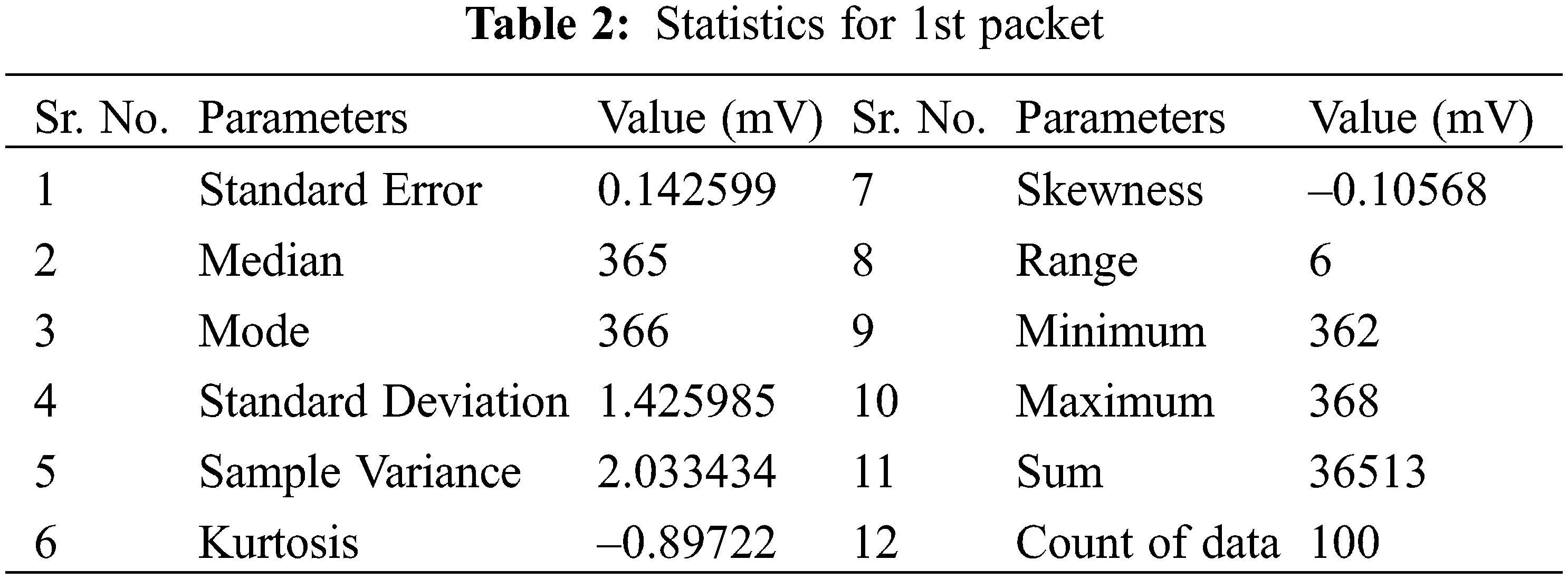
The statistical approach is used to examine the difference in a vibration signal for each of the tool category. An output of accelerometer, i.e., time and corresponding voltage was stored & read in MS-Excel. For each of the machining operation, roughly 5,000–5,100 values of voltage for consecutive time instances were observed. With an intention to detect the least variation in this signal, the whole response was split into packets. The size of a packet was kept as 100 data points. So, near about 50 packets were created for each tool condition. At this stage, descriptive stats for all packets were computed. The statistics for 1st packet of tool condition ‘GD’ are represented in Table 2.
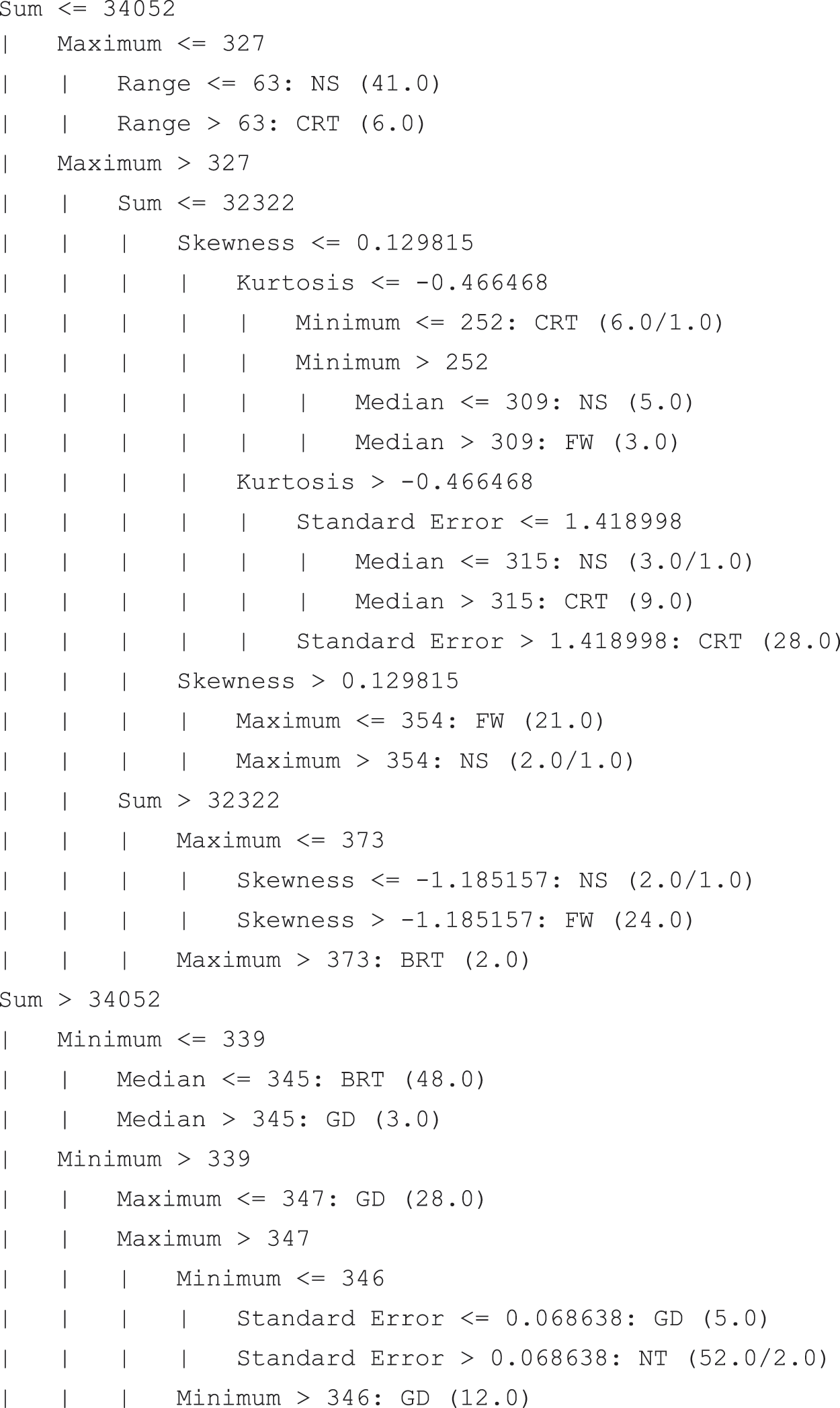
Once statistics are calculated, it is necessary to choose the parameters that exhibit differences relating to tool classes. The parameters which exhibit similarity for all tool classes must be removed to acquire accurate results. It is called ‘parameter selection’. Use of decision tree J48 is advocated here. The multiple binary rules-based model for categorization is designed using a decision tree and is presented.
• The manual observation for examining differences and similarity of each parameter is not possible hence the J48 algorithm can be employed.
• It was formulated by Ross Quinlan. Similar to others, C4.5 uses training data to construct a judgmental tree based on the principle of ‘entropy drop’ or ‘info gain’.
• The internal nodes signify features and the leaf nodes signify category.
• The J48 is considered as the most popular for the selection of salient features and categorization too [24].
Figs. 4a and 4b show a classification rule generated using the J48 decision tree selector. The 12 statistics mentioned in Table 2 were fed to the J48 algorithm out of which only 8 were selected by the algorithm for categorization. In other words, 8 out of 12 statistical features are significant for this particular set of data. The rule set generated is a simple If, else If loop. For instance, if the sum is less than or equal to 34052, then, the maximum is evaluated. If the maximum is less than or equal to 327, then, the range is evaluated. If the range value is lesser than or equal to 63, thus, a tool will be classified to be defective with nose wear. Similarly, the tree can be evaluated for other instances.
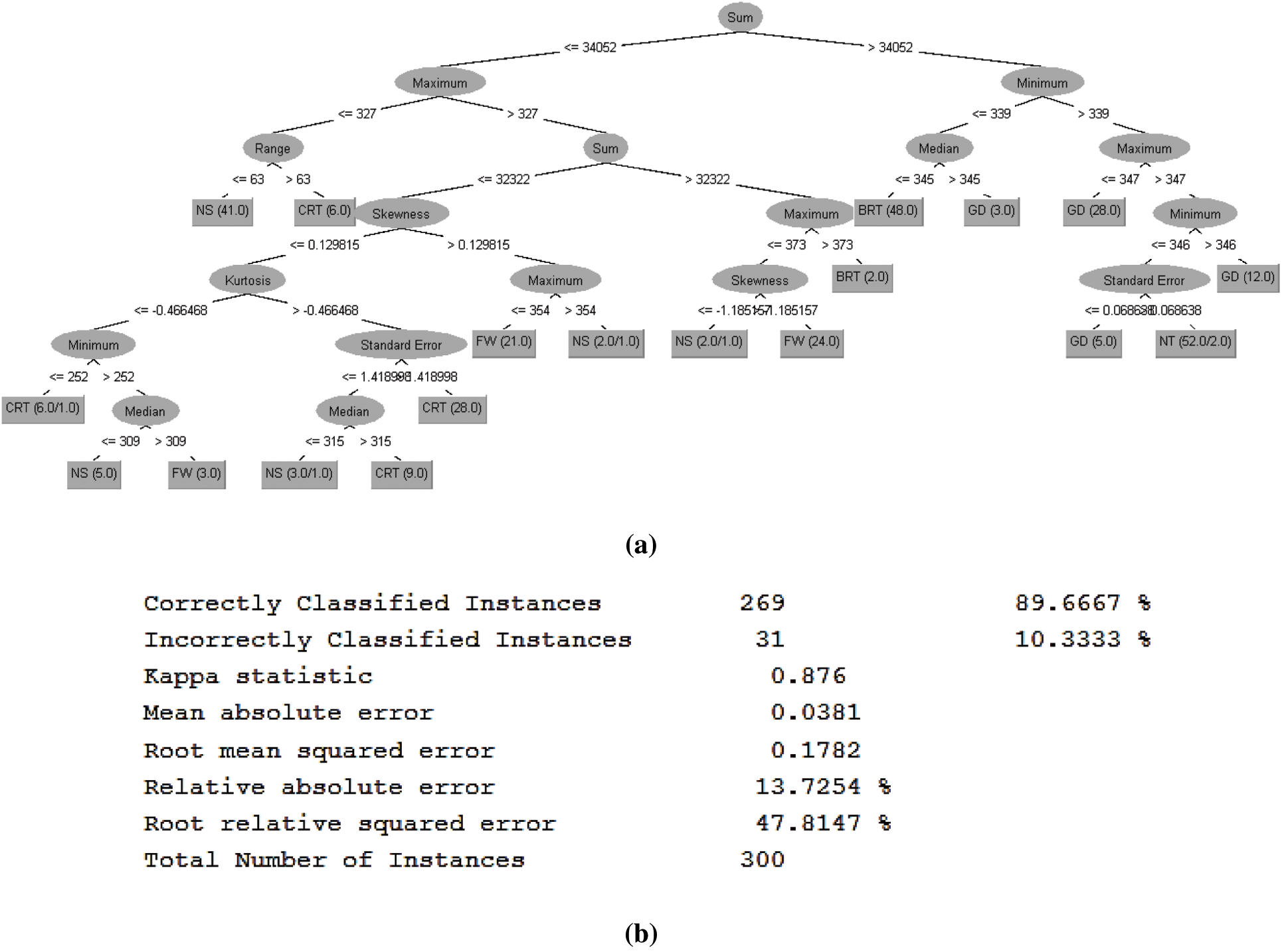
Figure 4: (a) Multiple binary rules based model for categorization using J48 algorithm; (b) Performance of J48 algorithm
In this section, various tree-based algorithms are used for the categorization of tool conditions. A decision tree algorithm is easy to build, easy to use, and easy to interpret. The classification accuracy using each tree algorithm is different, though, not necessarily unique. Hence 4 different types of tree-based algorithms are used in this investigation. The principle of working of each one is explained herein.
3.3.1 Random Tree Classifier (RTC)
It was first presented by Leo Breiman and Adele Cutler. It is based on a simple effective idea of generating a tree by selecting the best set of attributes at each node. It randomly selects a subset of predictors provided via feature vector making each node input unique. Though, after the introduction of Random Trees (Forest), the use of random tree became limited [25].
3.3.2 Logistic Model Tree Classifier (LMTC)
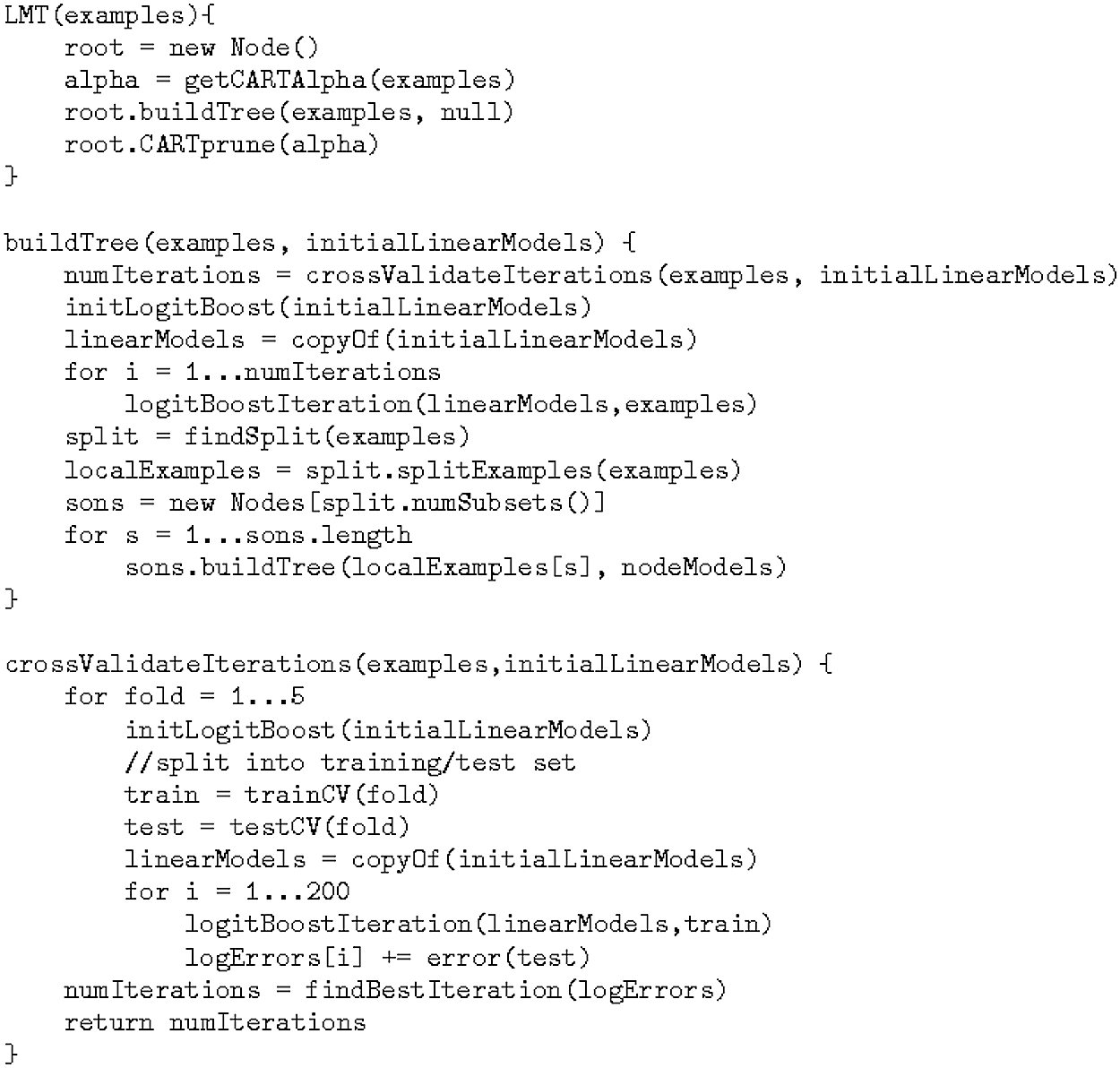
LMTC was first introduced by Niels Landwehr, Mark Hall, and Eibe Frank in 2003. It is a precise mixture of logistic regression and tree learning. It creates a simple binary rule sets as same as decision tree in addition to logistic type of regression at a leaf. An importance of executing logistic type of regression at the leaf is that it gives classification probability which is an important feature for any real-time application [26]. Fig. 5 depicts the flow of LMT induction.
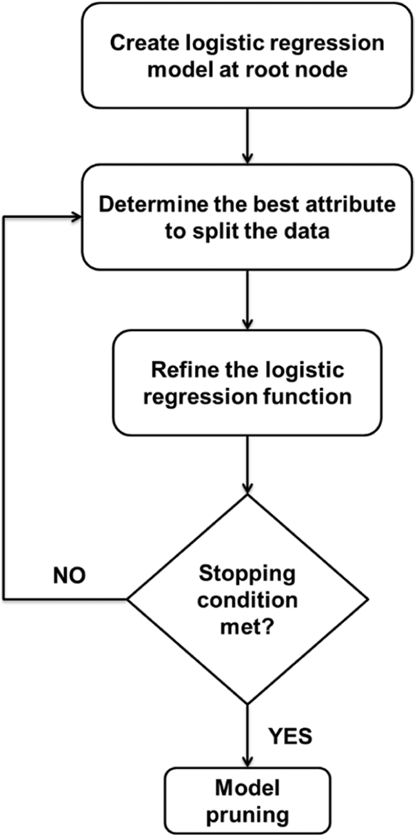
Figure 5: LMT induction [29,30]
3.3.3 Random Forest Classifier (RFC)
It integrates the simple principle of trees with flexible nature which results in improved accuracy. Fig. 6 depicts the difference between training of random forest & simple tree. Basically, it is inducted from a large group of de-correlated random trees. RFC creates many random trees and uses mode of the classes to make a decision. Random forest solves the problem of over-fitting and at the same time, it has the capability of handling large datasets with higher dimensionality [27]. Fig. 7 illustrates induction of decision tree and random forest separately.
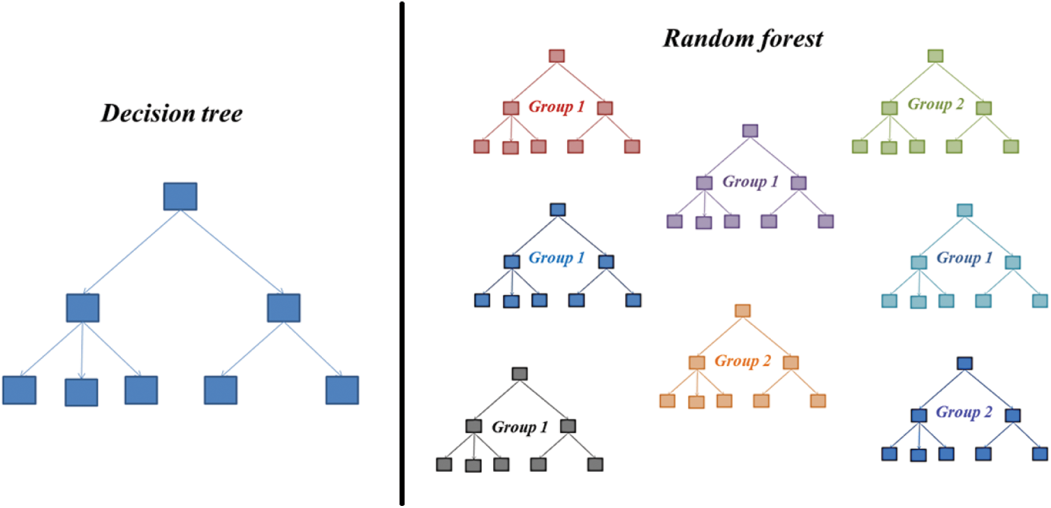
Figure 6: Random forest & simple tree [31]
Figure 7: Decision tree and random forest induction [32]
3.3.4 Reduced Error Pruning Tree Classifier (REPTC)
REPC creates a decision tree using information gain as the criteria to split nodes. Here, pruning is a procedure of modifying the DT to reduce the error in misclassification. This is achieved by generating a pruning set which provides an evaluation of rate of error on the test samples in future rather than on the same data used in training. REP Tree reduces over-fitting significantly [28]. The REP Tree procedure is explained here.
• Divide the data of training into separate pruning (33%) and training (66%) sets
• Design and start training of the tree
• Adopt bottom-up approach, i.e., start from leaves and check accuracy, if performance improves then start pruning of the test node
• How to size the accuracy? Use number of right vs. wrong classified samples in pruning set
• Carry on the examination on test nodes by bottom-up approach till nothing extra to be pruned
• Employ pruned tree model on separate testing set (not part of the pruning or training sets)
• In this way which is same as pruning regulations with Ripper, one can train the model
The statistical approach has been very popular for examining the difference in a vibration signals of each of the tool category [33–40] and thus used herein. The time-domain response of vibration was studied using a statistical approach. The J48 algorithm was used to extract significant facts. After this, various tree-based algorithms are used for the categorization of tool conditions. The feature extraction, selection, and classification are explained in the next subsections. The categorization of tool condition has been performed using various tree-based algorithms and the results are discussed using matrix and various parameters. The number of samples used for training was 40, testing 10, and validation 50.
4.1 Random Tree Classifier (RTC)
Random tree exhibited an accuracy of 87.3333%, i.e., for about 87.3333% of the packets the predicted class and actual class were same. The classification matrix gives a detailed report as shown in Fig. 8. Each class consisted of total 50 packets. The observations from matrix are made and stated here.
• Good: 47 packets were correctly classified, 3 were incorrectly classified; 2 as Notching and 1 as Broken tip.
• Notching: 48 packets were correctly classified and 2 were incorrectly classified as Good.
• Worn Nose: 42 packets were correctly classified and remaining 8 were incorrectly classified; 5 as Worn Flank and 3 as Cratering.
• Worn Flank: 34 packets were correctly classified, 16 were incorrectly classified; 5 as Worn nose, 1 as Broken tip and 10 as Cratering.
• Broken tip: 46 packets were correctly classified and 4 were incorrectly classified; 1 as Good, 1 as Worn nose, 1 as Worn Flank and 1 as Cratering.
• Cratering: 45 packets were correctly classified and 5 were incorrectly classified; 1 as Good, 2 as Worn nose, 1 as Worn Flank and 1 as Broken tip.
Figure 8: Results for random tree
4.2 Random Forest Classifier (RFC)
Random Forest tree exhibited an accuracy of 92.6667%, i.e., for about 92.6667% of the packets the predicted class and actual class were same. The observations from matrix are made & depicted in Fig. 9.
Figure 9: Results for random forest
• Good: 45 packets were correctly classified, 5 were incorrectly classified; 2 as Notching and 3 as Broken tip.
• Notching: 49 packets were correctly classified and 1 was incorrectly classified as Good.
• Worn Nose: 45 packets were correctly classified and remaining 5 were incorrectly classified; 1 as Worn Flank, 1 as Broken tip and 3 as Cratering.
• Worn Flank: 46 packets were correctly classified, 4 were incorrectly classified; 1 as Worn nose, 2 as Broken tip and 1 as Cratering.
• Broken tip: 48 packets were correctly classified and 2 were incorrectly classified as Worn Flank.
• Cratering: 45 packets were correctly classified and 5 were incorrectly classified; 1 as Worn nose and 4 as Worn Flank.
Random Forest integrates the simple principle of trees with flexible nature which results in improved accuracy. While, Random tree provides an accuracy of 87.33%, it is rather natural for random forest to give an accuracy of 92.66% which can be confirmed from the resulting confusion matrix.
4.3 Logistic Model Tree Classifier (LMTC)
LMTC exhibited an accuracy of 90%, i.e., for about 90% of the packets the predicted class and actual class were same. The observations from matrix are made and depicted in Fig. 10.
Figure 10: Results for LMT
• Good: 46 packets were correctly classified, 4 were incorrectly classified; 3 as Notching and 1 as Broken tip.
• Notching: 45 packets were correctly classified and 5 were incorrectly classified as Good.
• Worn Nose: 44 packets were correctly classified and remaining 6 were incorrectly classified; 3 as Worn Flank, 1 as Broken tip and 2 as Cratering.
• Worn Flank: 40 packets were correctly classified, 10 were incorrectly classified; 3 as Worn nose, 2 as Broken tip and 5 as Cratering.
• Broken tip: All of the 50 packets were correctly classified.
• Cratering: 45 packets were correctly classified and 5 were incorrectly classified; 3 as Worn nose and 2 as Worn Flank.
Owing to a precise mixture of logistic regression and tree learning, LMT is creates a simple binary rule sets as same as decision tree in addition to logistic type of regression at a leaf. This is the reason behind gaining the accuracy of 90% using k-fold cross validation test mode. LMTC thus regarded as a hybrid algorithm for classification of the data.
4.4 Reduced Error Pruning Tree Classifier (REPTC)
REP tree exhibited an accuracy of 87.3333%, i.e., for about 87.3333% of the packets the predicted class and actual class were same. The observations from matrix are made and depicted in Fig. 11.
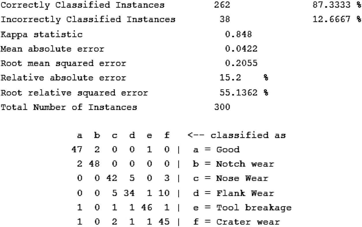
Figure 11: Results for REP tree
• Good: 47 packets were correctly classified, 3 were incorrectly classified; 2 as Notching and 1 as Broken tip.
• Notching: 48 packets were correctly classified and 2 were incorrectly classified as Good.
• Worn Nose: 42 packets were correctly classified and remaining 8 were incorrectly classified; 5 as Worn Flank and 3 as Cratering.
• Worn Flank: 34 packets were correctly classified, 16 were incorrectly classified; 5 as Worn nose, 1 as Broken tip and 10 as Cratering.
• Broken tip: 46 packets were correctly classified and 4 were incorrectly classified; 1 as Good, 1 as Worn nose, 1 as Worn Flank and 1 as Cratering.
• Cratering: 45 packets were correctly classified and 5 were incorrectly classified; 1 as Good, 2 as Worn nose, 1 as Worn Flank and 1 as Broken tip.
Amongst all algorithms, the Random Forest classifier found to exhibit the highest accuracy, i.e., 92.66%. Other tree algorithms also exhibited accuracy above 85%. This accuracy was found based on the assessment of ‘cross-validation’ of 10 splits so the trained model is considered as reliable. The detailed accuracy of Random Forest with the help of True positive rate, False positive rate, ROC, Precision, Recall, MCC, F-measure, etc., is illustrated in the Fig. 12.
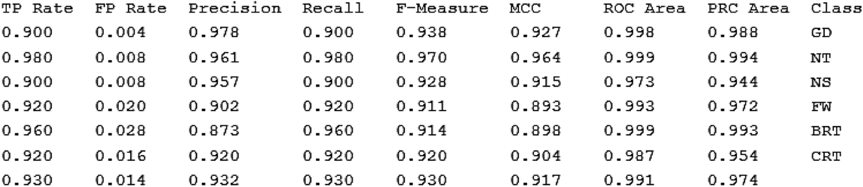
Figure 12: Detailed accuracy of random forest tree
• The TP, i.e., true positive states how correctly the trained data estimates prediction of the true category
• The FP, i.e., false positive states how wrongly the trained data estimates prediction of the true category
• The Matthews correlation coefficient (MCC) indicates the quality of binary classifications
• The precision indicates the % of correctly classified results among the reclaimed ones
• The recall indicates the % of total relevant results correctly categorized
• The F measure indicates the weighted harmonic mean of precision and recall
• The Receiver Operating Characteristics (ROC) area indicates in general quality of the classifiers
• It is a graph of TP portion (i.e., sensitivity) on x axis and FP portion (i.e., 1–specificity) on y axis
• The Precision Recall Curve (PRC) area is a graph of precision on x axis and recall on Y axis
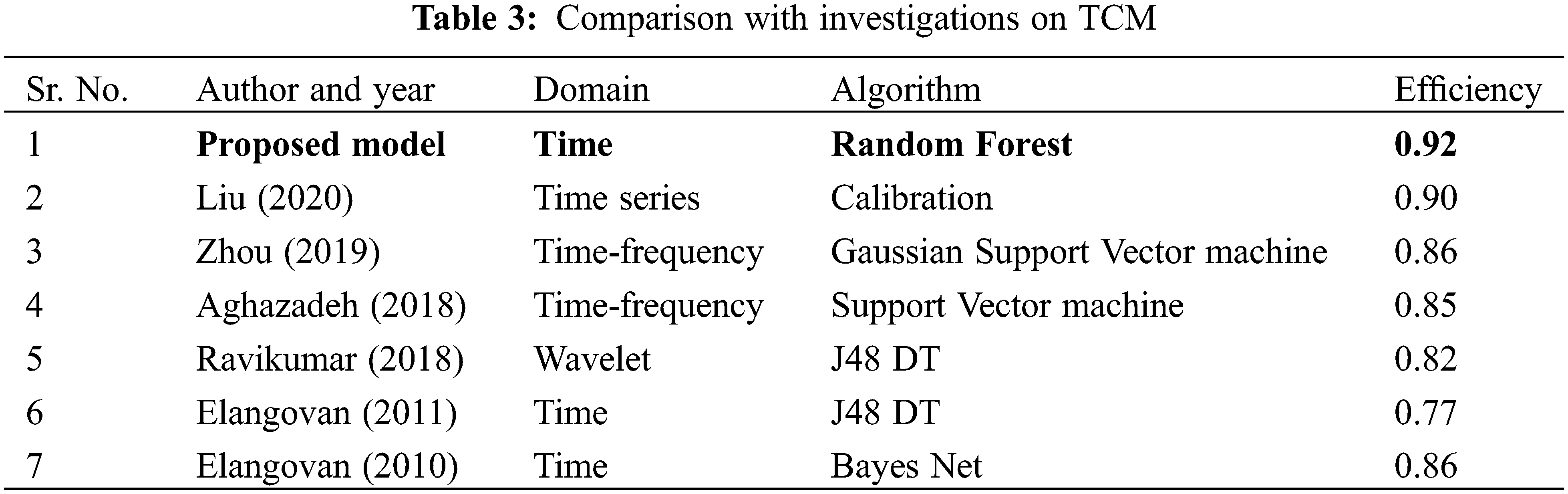
Also errors are presented in Fig. 13. Hence the methodology adopted for the classification of tool faults in turning is found suitable and appropriate. The proposed framework is evaluated w.r.t. others contribution (literature) and shown in Table 3.
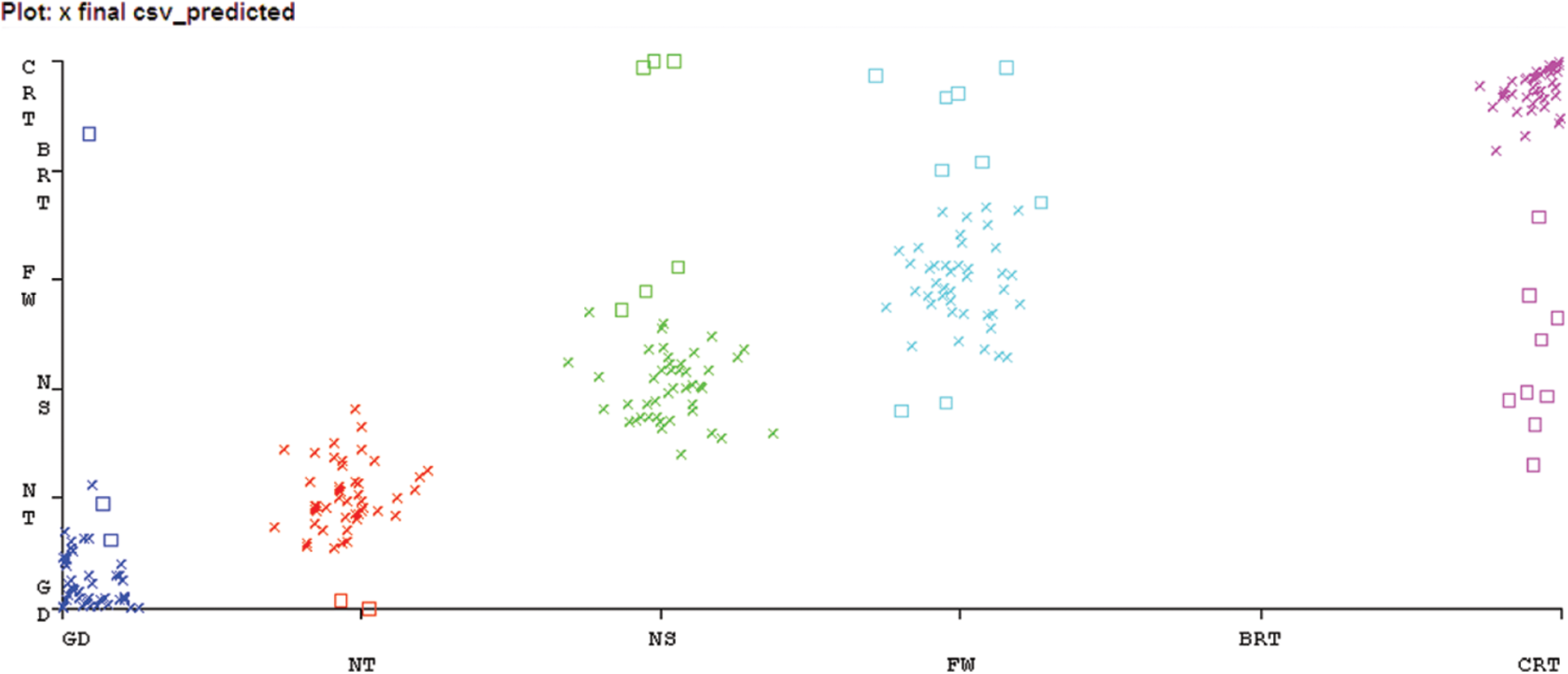
Figure 13: Representation of errors
The traditional TMS followed by the ML analysis was well obtained for the classification of tool faults in turning. In the current study, investigation on the single point cutting tool is carried out while turning a stainless steel (SS) workpeice on the manual lathe trainer. The vibrations developed during this activity are examined for failure-free and various failure states of a tool. The statistical modeling is then incorporated to trace vital signs from vibration signals. The multiple-binary-rule-based model for categorization is designed using the decision tree. Lastly, various tree-based algorithms are used for the categorization of tool conditions.
• The vibrations progressed during machining were found suitable for associating it with the various faults the tool. The statistical modeling showed vital signs from vibration signals
• The Random Forest classifier (RFC) found to exhibit the highest accuracy, i.e., 92.66%. Other tree algorithms also exhibited accuracy above 85%. Hence tree-based classifiers found appropriate for the classifying the tool faults
• This study would be helpful for onboard condition monitoring. The investigation for the incorporation of open-source software with low-cost instrumentation for condition-based monitoring can be done in the near future so that cost-effective solutions can be proposed
This study is limited to classifying of tool faults in correlation with the vibration data obtained from fixed machining parameters. If any of these parameters, viz. feed, cutting depth and speed is altered; the condition of tool is directly affected. This variation makes a wide range of data corresponding to more stages of failures in the same class available to the trained model. This may result in misclassification. Such misclassification can be avoided by carrying out a study that deals with various values of input parameters and phases of tool faults in a class, to generate a more accurate classification model.
Acknowledgement: The authors would like to acknowledge Sinhgad Technical Education Society, Dr. V. V. Dixit, Director—RMDSTIC & Principal—RMDSSOE and Dr. S. S. Mulik Professor & Dean Academics—STES’s RMD Sinhgad School of Engineering, Warje, Pune for providing facility to carry out experimental study.
Funding Statement: The authors received no specific funding for this study.
Conflicts of Interest: The authors declare that they have no conflicts of interest to report regarding the present study.
1. Knight, W. A., Boothroyd, G. (2018). Fundamentals of metal machining and machine tools, vol. 3, pp. 1–75. Boca Raton: CRC Press, Taylor & Francis Group. [Google Scholar]
2. Botsaris, P. N., Tsanakas, J. A. (2008). State-of-the-art in methods applied to tool condition monitoring (TCM) in unmanned machining operations: A review. The Proceedings of the International Conference of COMADEM, pp. 73–87. Prague, Czech Republic. [Google Scholar]
3. Shewale, M. S., Mulik, S. S., Deshmukh, S. P., Patange, A. D. (2018). A novel health monitoring system. Proceedings of 2nd International Conference on Data Engineering and Communication Technology Advances in Intelligent Systems and Computing, vol. 828, pp. 461–468. Singapore, Springer. [Google Scholar]
4. Patange, A. D., Jegadeeshwaran, R., Dhobale, N. C. (2019). Milling cutter condition monitoring using machine learning approach. IOP Conference Series: Materials Science and Engineering, 624(1), 1–5. DOI 10.1088/1757-899X/624/1/012030. [Google Scholar] [CrossRef]
5. Patange, A. D., Jegadeeshwaran, R. (2020). A machine learning approach for vibration-based multipoint tool insert health prediction on vertical machining centre (VMC). Measurement, 173. DOI 10.1016/j.measurement.2020.108649. [Google Scholar] [CrossRef]
6. Scheffer, C., Kratz, H., Heyns, P. S., Klocke, F. (2003). Development of a tool wear-monitoring system for hard turning. International Journal of Machine Tools and Manufacture, 43(10), 973–985. DOI 10.1016/S0890-6955(03)00110-X. [Google Scholar] [CrossRef]
7. Kopa, J., Sali, S. (2001). Tool wear monitoring during the turning process. Journal of Materials Processing Technology, 113(1), 312–316. DOI 10.1016/S0924-0136(01)00621-5. [Google Scholar] [CrossRef]
8. Dolinsek, S., Kopa, J. (2006). Mechanism and types of tool wear: Particularities in advanced cutting materials. Journal of Achievements in Materials and Manufacturing Engineering, 19(1), 11–18. [Google Scholar]
9. Siddhpura, M., Paurobally, R. (2013). A review of worn flank prediction methods for tool condition monitoring in a turning process. International Journal of Advanced Manufacturing Technology, 65, 371–393. DOI 10.1007/s00170-012-4177-1. [Google Scholar] [CrossRef]
10. Rehorn, A. G., Jiang, J., Orban, P. E. (2005). State-of-the-art methods and results in tool condition monitoring: A review. International Journal of Advanced Manufacturing Technology, 26, 693–710. DOI 10.1007/s00170-004-2038-2. [Google Scholar] [CrossRef]
11. Byrne, G., Dornfeld, D., Inasaki, I., Ketteler, G., Konig, W. et al. (1995). Tool condition monitoring (TCM)–The status of research and industrial application. CIRP Annals-Manufacturing Technology, 44(2), 541–567. DOI 10.1016/S0007-8506(07)60503-4. [Google Scholar] [CrossRef]
12. Abukhshim, N. A., Mativenga, P. T., Sheikh, M. A. (2006). Heat generation and temperature prediction in metal cutting: A review and implications for high speed machining. International Journal of Machine Tools and Manufacture, 46, 782–800. DOI 10.1016/j.ijmachtools.2005.07.024. [Google Scholar] [CrossRef]
13. Jantunen, E. (2002). A summary of methods applied to tool condition monitoring in drilling. International Journal of Machine Tools and Manufacture, 42(9), 997–1010. DOI 10.1016/S0890-6955(02)00040-8. [Google Scholar] [CrossRef]
14. Leo, R. (2003). Monitoring improves machine up time and shop efficiency. Production Machining. https://www.productionmachining.com/articles/monitoring-improves-machine-up-time-and-shop-efficiency. [Google Scholar]
15. Li, X. (2001). Real-time tool wear condition monitoring in turning. International Journal of Production Research, 39(5), 981–992. DOI 10.1080/00207540010005745. [Google Scholar] [CrossRef]
16. Nayfeh, T. H., Eyada, O. K., Duke, J. C. (1995). An integrated ultrasonic sensor for monitoring gradual wear on-line during turning operations. International Journal of Machine Tools and Manufacture, 35(10), 1385–1395. DOI 10.1016/0890-6955(94)00126-5. [Google Scholar] [CrossRef]
17. Painuli, S., Elangovan, M., Sugumaran, V. (2014). Tool condition monitoring using K-star algorithm. Expert Systems with Applications, 41(6), 2638–2643. DOI 10.1016/j.eswa.2013.11.005. [Google Scholar] [CrossRef]
18. Elangovan, M., Ramachandran, K. I., Sugumaran, V. (2010). Studies on Bayes classifier for condition monitoring of single point carbide tipped tool based on statistical and histogram features. Expert Systems with Applications, 37(3), 2059–2065. DOI 10.1016/j.eswa.2009.06.103. [Google Scholar] [CrossRef]
19. Thangarasu, S. K., Shankar, S., Mohanraj, T., Devendran, K. (2020). Tool wear prediction in hard turning of EN8 steel using cutting force and surface roughness with artificial neural network. Proceedings of the Institution of Mechanical Engineers, Part C: Journal of Mechanical Engineering Science, 234(1), 329–342. DOI 10.1177/0954406219873932. [Google Scholar] [CrossRef]
20. Mohanraj, T., Shankar, S., Rajasekar, R., Sakthivel, N. R., Pramanik, A. (2020). Tool condition monitoring techniques in milling process—A review. Journal of Materials Research and Technology, 9(1), 1032–1042. DOI 10.1016/j.jmrt.2019.10.031. [Google Scholar] [CrossRef]
21. Mohanraj, T., Jayanthi, Y., Krishnan, H., Aravind, R. S., Yameni, R. (2021). Development of tool condition monitoring system in end milling process using wavelet features and Hoelder’s exponent with machine learning algorithms. Measurement, 173. DOI 10.1016/j.measurement.2020.108671. [Google Scholar] [CrossRef]
22. Nalavade, S. P., Patange, A. D., Prabhune, C. L., Mulik, S. S. (2018). Development of 12 channel temperature acquisition system for heat exchanger using MAX6675 and Arduino interface. In: Lecture notes in mechanical engineering, vol. 1, pp. 119–125. Springer. DOI 10.1007/978-981-13-2697-4_13. [Google Scholar] [CrossRef]
23. Patange, A. D., Bewoor, A. K., Deshmukh, S. P., Mulik, S. S., Pardeshi, S. S. et al. (2019). Improving program outcome attainments using project based learning approach for: UG course-mechatronics. Journal of Engineering Education Transformations, 33(1), 1–8. DOI 10.16920/jeet/2019/v33i1/148977. [Google Scholar] [CrossRef]
24. Kingsford, C., Salzberg, S. L. (2008). What are decision trees? Nature Biotechnology, 26(9), 1011–1013. DOI 10.1038/nbt0908-1011. [Google Scholar] [CrossRef]
25. Barros, R. C., Basgalupp, M. P., Freitas, A. A., de Carvalho, A. C. P. L. F. (2014). Evolutionary design of decision-tree algorithms tailored to microarray gene expression data sets. IEEE Transactions on Evolutionary Computation, 18(6), 873–892. DOI 10.1109/TEVC.2013.2291813. [Google Scholar] [CrossRef]
26. Colkesen, I., Kavzoglu, T. (2017). The use of logistic model tree (LMT) for pixel and object-based classifications using high resolution World view-2 imagery. Geocarto International, 32, 71–86. DOI 10.1080/10106049.2015.1128486. [Google Scholar] [CrossRef]
27. Chen, W., Zhang, S., Li, R., Shahabi, H. (2018). Performance evaluation of the GIS-based data mining techniques of best-first decision tree, random forest, and naïve Bayes tree for landslide susceptibility modeling. Science of the Total Environment, 44, 1006–1018. DOI 10.1016/j.scitotenv.2018.06.389. [Google Scholar] [CrossRef]
28. Tanha, J., Someren, M. V., Afsarmanesh, H. (2017). Semi-supervised self-training for decision tree classifiers. International Journal of Machine Learning and Cybernetics, 8(1), 355–370. DOI 10.1007/s13042-015-0328-7. [Google Scholar] [CrossRef]
29. Beretta, S., Castelli, M., Gonçalves, I., Kel, I., Giansanti, V. et al. (2018). Improving eQTL analysis using a machine learning approach for data integration: A logistic model tree solution. Journal of Computational Biology, 25(10), 1091–1105. DOI 10.1089/cmb.2017.0167. [Google Scholar] [CrossRef]
30. Landwehr, N., Hall, M., Frank, E. (2005). Logistic model trees. Machine Learning, 59(1–2), 161–205. DOI 10.1007/s10994-005-0466-3. [Google Scholar] [CrossRef]
31. Khairnar, A., Abhishek, P., Pardeshi, S., Jegadeeshwaran, R. (2021). Supervision of carbide tool condition by training of vibration-based statistical model using boosted trees ensemble. International Journal of Performability Engineering, 17(2), 229–240. DOI 10.23940/ijpe.21.02.p7.229240. [Google Scholar] [CrossRef]
32. Khade, H. S., Patange, A. D., Pardeshi, S. S., Jegadeeshwaran, R. (2021). Design of bagged tree ensemble for carbide coated inserts fault diagnosis. Materials Today: Proceedings, 46(2), 1283–1289. DOI 10.1016/j.matpr.2021.02.128. [Google Scholar] [CrossRef]
33. Patange, A. D., Jegadeeshwaran, R. (2021). Review on tool condition classification in milling: A machine learning approach. Materials Today: Proceedings, 46(2), 1106–1115. DOI 10.1016/j.matpr.2015.07.317. [Google Scholar] [CrossRef]
34. Sonali, S. P., Sujit, S. P., Nikhil, P., Abhishek, D. P. (2022). Cutting tool condition monitoring using a deep learning-based artificial neural network. International Journal of Performability Engineering, 18(1), 37–46. DOI 10.23940/ijpe.22.01.p5.3746. [Google Scholar] [CrossRef]
35. Tambake, N. R., Deshmukh, B. B., Patange, A. D. (2021). Data driven cutting tool fault diagnosis system using machine learning approach: A review. Journal of Physics: Conference Series, 1969, 1–14. DOI 10.1088/1742-6596/1969/1/012049. [Google Scholar] [CrossRef]
36. Bajaj, N. S., Patange, A. D., Jegadeeshwaran, R., Kulkarni, K. A., Ghatpande, R. S. et al. (2022). A Bayesian optimized discriminant analysis model for condition monitoring of face milling cutter using vibration datasets. Journal of Nondestructive Evaluation, Diagnostics and Prognostics of Engineering Systems, 5(2). DOI 10.1115/1.4051696. [Google Scholar] [CrossRef]
37. Medhi, A. M., Patange, A. D., Pardeshi, S. S., Jegadeeshwaran, R., Kuntoglu, M. (2022). Overview of contemporary systems driven by open-design movement. https://arxiv.org/abs/2201.05698. [Google Scholar]
38. Deo, T. Y., Patange, A. D., Pardeshi S. S., Jegadeeshwaran, R., Khairnar A. N. et al. (2022). A white-box SVM framework and its swarm-based optimization for supervision of toothed milling cutter through characterization of spindle vibrations. https://arxiv.org/abs/2112.08421. [Google Scholar]
39. Patil, S. S., Pardeshi, S. S., Patange, A. D., Jegadeeshwaran, R. (2021). Deep learning algorithms for tool condition monitoring in milling: A review. Journal of Physics: Conference Series, 1969, 1–10. DOI 10.1088/1742-6596/1969/1/012039. [Google Scholar] [CrossRef]
40. Patange Abhishek, D., Jegadeeshwaran, R. (2020). Application of Bayesian family classifiers for cutting tool inserts health monitoring on CNC milling. International Journal of Prognostics and Health Management, 11(2). DOI 10.36001/ijphm.2020.v11i2.2929. [Google Scholar] [CrossRef]
Annexure I: Algorithm for LMT Induction [29,30]
Annexure II: Multiple binary rules based model for categorization using J48 algorithm
 | This work is licensed under a Creative Commons Attribution 4.0 International License, which permits unrestricted use, distribution, and reproduction in any medium, provided the original work is properly cited. |