DOI:10.32604/cmc.2021.016036
| Computers, Materials & Continua DOI:10.32604/cmc.2021.016036 | |
| Article |
Reconstructing the Time-Dependent Thermal Coefficient in 2D Free Boundary Problems
Department of Mathematics, College of Science, Jazan University, Jazan, Saudi Arabia
*Corresponding Author: M. J. Huntul. Email: mhantool@jazanu.edu.sa
Received: 19 December 2020; Accepted: 19 January 2021
Abstract: The inverse problem of reconstructing the time-dependent thermal conductivity and free boundary coefficients along with the temperature in a two-dimensional parabolic equation with initial and boundary conditions and additional measurements is, for the first time, numerically investigated. This inverse problem appears extensively in the modelling of various phenomena in engineering and physics. For instance, steel annealing, vacuum-arc welding, fusion welding, continuous casting, metallurgy, aircraft, oil and gas production during drilling and operation of wells. From literature we already know that this inverse problem has a unique solution. However, the problem is still ill-posed by being unstable to noise in the input data. For the numerical realization, we apply the alternating direction explicit method along with the Tikhonov regularization to find a stable and accurate numerical solution of finite differences. The root mean square error (rmse) values for various noise levels p for both smooth and non-smooth continuous time-dependent coefficients Examples are compared. The resulting nonlinear minimization problem is solved numerically using the MATLAB subroutine lsqnonlin. Both exact and numerically simulated noisy input data are inverted. Numerical results presented for two examples show the efficiency of the computational method and the accuracy and stability of the numerical solution even in the presence of noise in the input data.
Keywords: Inverse identification problem; two-dimensional parabolic equation; free boundary; Tikhonov regularization; nonlinear optimization
Free boundary problems for the parabolic partial differential equations have significant applications in various fields of engineering, physics, chemistry, see [1–5] to mention only a few. A Stefan problem is a moving boundary value problem that concerns the distribution of heat in a period of transforming medium. The authors of [6] considered two fairly different free boundary problems of nonlinear diffusion. Chen et al. [7] recast the formulation of various shock diffraction/reflection problems as a free boundary problem. Shidfar et al. [8] studied the inverse moving boundary problem using the least-squares method. In [9], the authors investigated the numerical solution of inverse Stefan problems using the method of fundamental solutions. Recently, the authors of [10] numerically solved the inverse heat problems of determining the time-dependent coefficients with free boundaries.
There is also an analysis of a one-dimensional inverse problem of reconstructing the timewise heat source with a moving boundary [11]. The authors in [12] estimated free boundary coming from two new scenarios, aggregation processes and nonlocal diffusion. Snitko [13,14], theoretically, and Huntul [15], numerically, investigated the inverse problem of determining the time-dependent reaction coefficient in a two-dimensional parabolic problem with a free boundary.
The challenge associated with free boundary problems arises from the finding that the solution domain is unknown. Only a few studies focus on the time-dependent free boundary in higher dimensions [16–19]. These papers are theoretical and very important because they present conditions for the unique solvability of the unknown coefficients.
This work examines the inverse problem to recover the time-dependent thermal conductivity coefficient and free boundaries from the heat flux and the nonlocal integral observations as over-specification conditions. The inverse problem presented in this paper has already been showed to be locally uniquely solvable by Barans’ka et al. [20], but no numerical determination has been realised so far, therefore, the main goal of this work is to attempt numerical solution of this problem.
The arrangement of this paper is systematized as follows. Section 2 describes the formulations of the inverse problem. The solution of the direct problem using the alternating direction explicit (ADE) method is presented in Section 3. The ADE direct solver is coupled with the Tikhonov regularization method in Section 4. In Section 5, computational results and discussions are presented. Finally, Section 6 highlights the conclusions.
2 Formulation of the Inverse Problem
Consider the inverse problem of reconstructing time-dependent thermal conductivity coefficient a(t) > 0, and the free boundaries l(t) > 0 and h(t) > 0 in the two-dimensional parabolic equation

where  is a known heat source,
  is the unknown temperature in the moving domain
  , with the initial condition

where l0 = l(0) and h0 = h(0) are given positive numbers, the Dirichlet boundary conditions


and the over-specification conditions

where Y0 is belong to the interval 


where  and
and  for
for  are given functions. The function
  in Eq. (5) represents heat flux boundary condition. The function
  in Eq. (6) corresponds to the specification of mass/energy, [21,22], whilst the function
  in Eq. (7) represents the first-order moment specification, [23].
Introducing the new variables y1 = x1/l(t) and y2 = x2/h(t), see [20], we recast the problem given by Eqs. (1) to (7) into the problem given below for the unknowns l(t), h(t), a(t) and  , namely,

in the fixed domain 


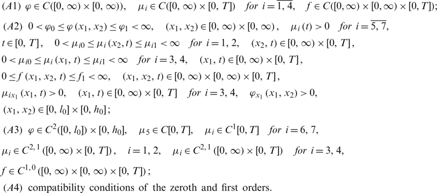
The existence and uniqueness of solution of the inverse problem Eqs. (8) to (14) has been established in [20] and read as follows.
Theorem 1 Suppose that the following assumptions are satisfied:
Then, it is possible to indicate a time  , determined by the input data, such that there exists a solution
  with l(t) > 0, h(t) > 0, a(t) > 0 for
  , to problem Eqs. (8) to (14).
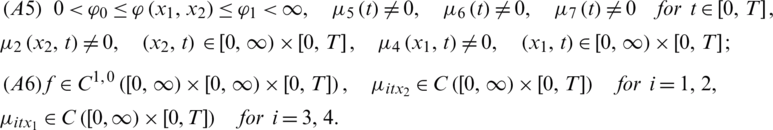
Theorem 2 Suppose that the following conditions are fulfilled:
Then, it is possible to indicate a time  , determined by the input data, such that problem Eqs. (8) to (14) has at most one solution
  with l(t) > 0, h(t) > 0, a(t) > 0 for
  .
.
3 Numerical Solution of the Forward Problem
Consider the direct (forward) problem Eqs. (8) to (11). When l(t), h(t), a(t),  ,
,  , for
, for  and
and  are given in the direct problem
  is to be found along with the quantities of interest
  for
for  . Denote
  , l(tn) = ln, h(tn) = hn, a(tn) = an and
  , where
  ,
,  ,
,  ,
,  ,
,  ,
,  ,
,  ,
,  ,
,  .
.
The ADE method, [3,24], which is unconditionally stable, is described for solving numerically the direct problem Eqs. (8) to (11). Let  and
and  satisfy


where
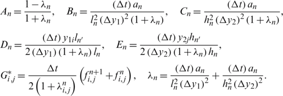
In the above expression, we approximate the derivatives of l(t) and h(t) as


Furthermore, let the  and
and  also satisfy the initial and boundary conditions Eqs. (9) to (11), namely,


Once  and
and  have been obtained, the solution for the direct problem Eqs. (8) to (11) is computed by

The heat flux in Eq. (12) can be approximated using the second-order FDM as follows.

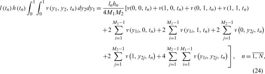
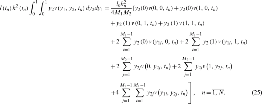
The integrals in Eqs. (13) and (14) can be calculated using the trapezoidal rule as follows:
4 Numerical Solution of the Inverse Problem
In this section, our aim is to obtain stable and accurate reconstructions of the free boundary l(t), h(t), the thermal conductivity a(t) together with the temperature  , satisfying Eqs. (8) to (14). The inverse problem can be formulated as a nonlinear least-squares minimization of the least-squares objective function given by
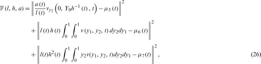
or, in discretizations form
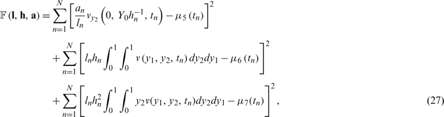
where  solves Eqs. (8) to (11) for given
  , respectively. The minimization of the function Eq. (27) is performed using the MATLAB subroutine
  [25].
[25].
The inverse problem given by Eqs. (8) to (14) is solved subject to both analytical and noisy (perturbed) measurements Eqs. (12) to (14). The perturbed data are numerically formulated as follows

where  are random variables with mean zero and standard deviations
  , given by

where p represents the percentage of noise. We use the MATLAB function  to generate the random variables
  as follows:

In the case of perturbed data Eq. (28), we replace in Eq. (27)  by
by  for
for  .
.
5 Numerical Results and Discussion
The accuracy is measured by rmse:


Let us take T = 1, for simplicity. The lower bounds and upper bounds for l(t) > 0, h(t) > 0 and a(t) > 0 are 10−9 for (LB) and 102 for (UB), respectively.
Consider the inverse problem given by Eqs. (1) to (7), with the smooth unknown timewise terms l(t), h(t) and a(t), and we solve it with:
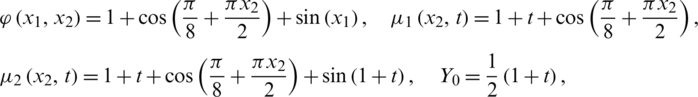
We observe that the conditions (A1)–(A6) of Theorems 1 and 2 are fulfilled and thus, the uniqueness condition of the solution is guaranteed. It can be easily verified that the analytical solution of Eqs. (1) to (4) is

and

Also,

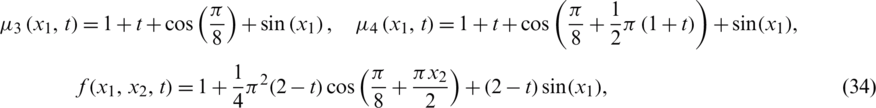
First, let us solve the forward problem Eqs. (1) to (4) with the input data (34) when l(t), h(t), a(t) are known and given by Eq. (37). Tab. 1 reveals that the exact and approximate solutions for Eqs. (12) to (14), which exactly is given by Eq. (35), obtained with number of grids M1 = M2 = 10 and  , are in good agreement. The analytical Eq. (38) and approximate solutions for
  is plotted in Fig. 1. It is clear from Tab. 1 and Fig. 1 that the accuracy of the approximate solution increases, as the mesh sizes decreases.
Table 1: The numerical and analytical Eq. (35) solutions for  ,
,  , with M1 = M2 = 10 and various
  , for direct problem

Figure 1: The solutions  and absolute errors with M1 = M2 = 10 for: (a) N = 20, (b) N = 40 and (c) N = 80, for direct problem
In the problem Eqs. (8) to (14), we take the initial guesses for  and
and  , as follows:

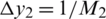
We take a mesh size with M1 = M2 = 10, N = 40 and we start the examination for recovering the timewise terms l(t), h(t) and a(t), when p = 0 in the measurements Eqs. (12) to (14), as in Eq. (31). The function Eq. (27) is illustrated in Fig. 2a, where a convergence, which is monotonically decreasing, is obtained in 10 iterations to achieve a low specified tolerance of O(10−28). Figs. 2b–2d illustrates the corresponding approximate results for the functions l(t), h(t) and a(t). A good agreement between the analytical Eq. (37) and approximate solutions can be observed from these figures with rmse(l) = 4.4E −3, rmse(h) = 3.8E −3 and rmse(a) = 6.4E −3.
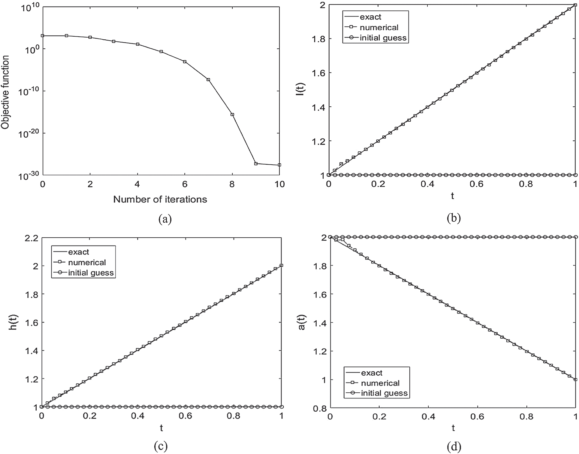
Figure 2: (a) The objective function Eq. (27) vs. the number of iterations, and the exact Eq. (37) and numerical solutions for: (b) l(t), (c) h(t) and (d) a(t), with no noise, for Example 1
Next, the stability of the numerical solution is investigated with respect to the noisy data Eq. (28). We include  noise to the over-determination conditions
  ,
,  and
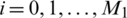
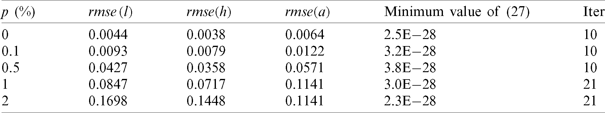
and  , as in Eq. (28) to test the stability. The function Eq. (27) is plotted in Fig. 3a and convergence is again rapidly achieved. The approximate results for l(t), h(t) and a(t) are depicted in Fig. 3. Accurate and stable results are obtained for l(t), h(t) and a(t) by observing Figs. 3b–3d and the rmse values, the minimum value of Eq. (27) at final iteration and the number of iterations are given in Tab. 2. As noise p is increased the approximate results for l(t), h(t) and a(t) start to build up oscillations. In order to retrieve stability, we penalise the function Eq. (27) by adding
 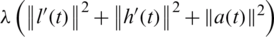 to it since the theory provide
  ,
,  and
and  , where
  is the Tikhonov’s regularization parameter to be chosen. Then, in discretised form of Tikhonov functional recasts as

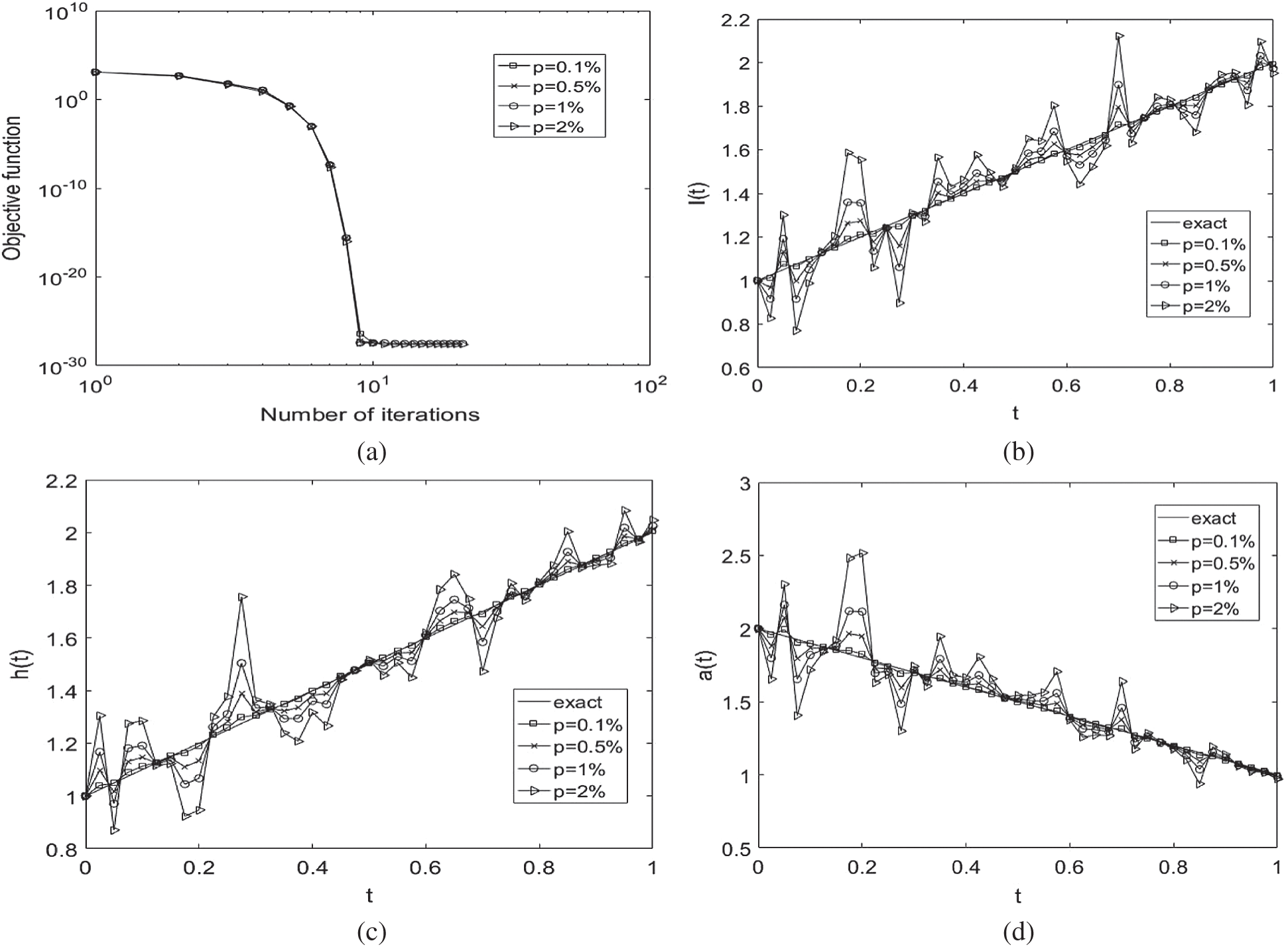
Figure 3: (a) The objective function Eq. (27) vs. the number of iterations, and the exact Eq. (37) and numerical solutions for: (b) l(t), (c) h(t) and (d) a(t), with  noise, for Example 1
Table 2: The values of rmse Eqs. (31) to (33), the function Eq. (27) at final iteration and the number of iterations, for  noise, for Example 1
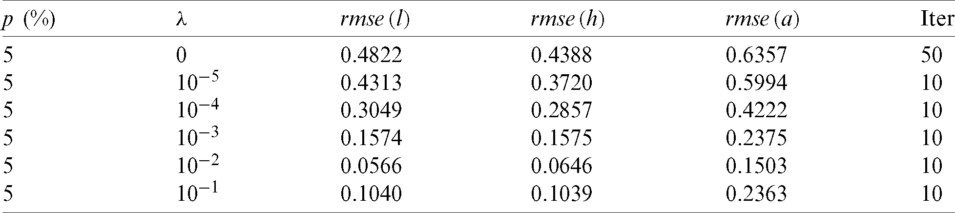
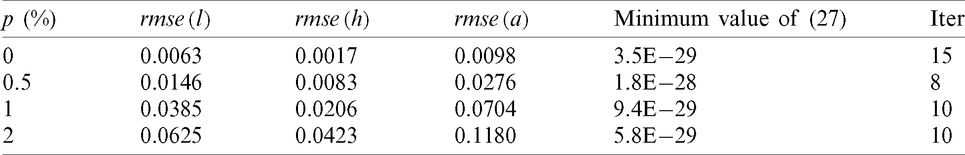
For  noise, Fig. 4 illustrates the analytical solution Eq. (37) and the approximate solutions obtained by minimizing the functional Eq. (40) for various regularization parameters. The
  values are
  ,
,  and
and  for
for  , see Tab. 3 for more information. It can be observed that the approximate unregularized solution obtained with
  demonstrates instability, however, on including regularization with
  to
to  , we get a stable solution which is consistent in accuracy with the
  noise desecrating the input data Eq. (28).
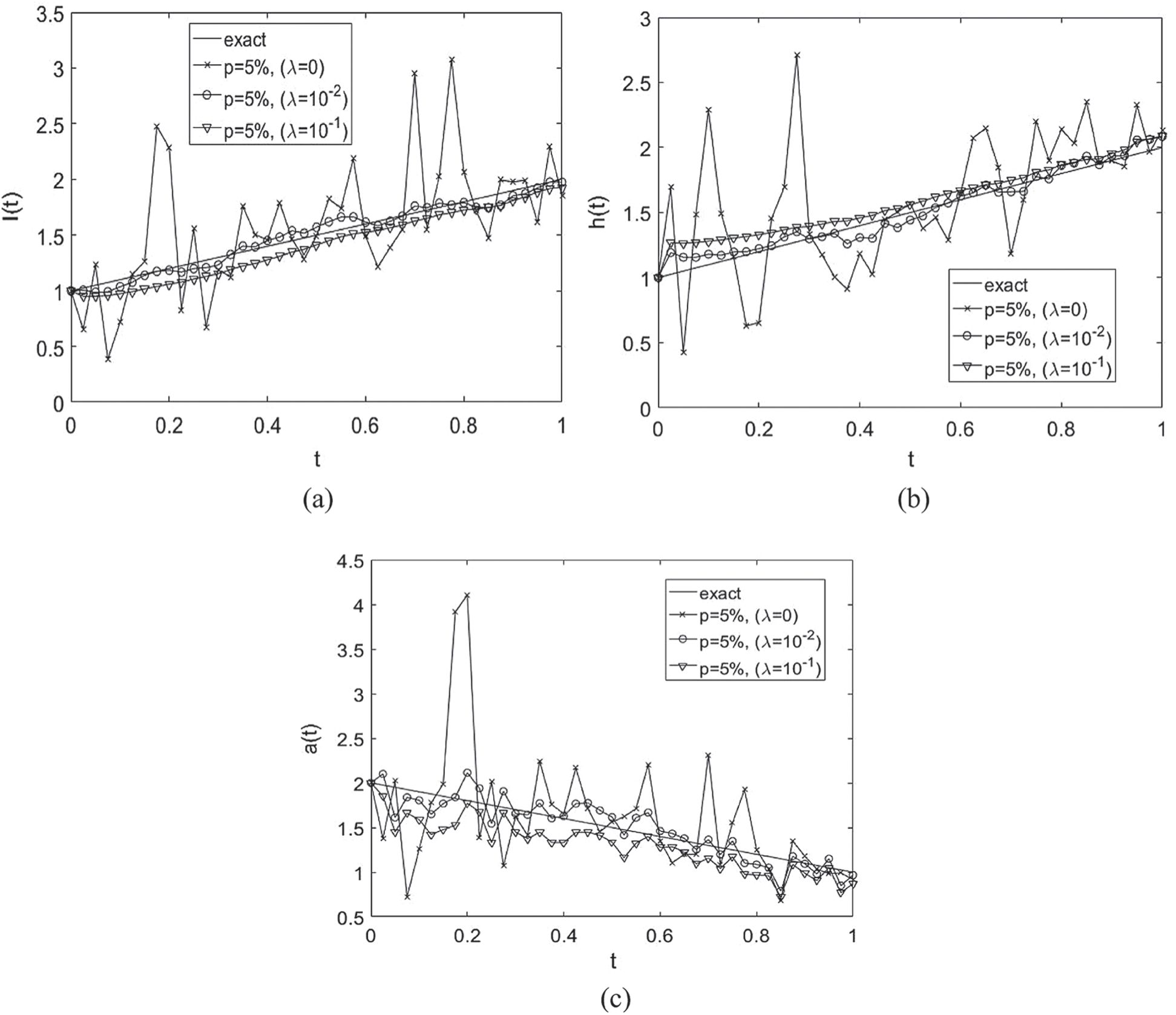
Figure 4: The numerical and analytical Eq. (37) solutions for: (a) l(t), (b) h(t) and (c) a(t), for  noise, with various
  , for Example 1
Table 3: The values of rmse Eqs. (31) to (33) and the number of iterations, for  noise, without and with regularization, for Example 1
The smooth timewise coefficients l(t), h(t), a(t) given by Eq. (37) has been recovered in previous example. In this example, let us examine the numerical scheme for recovering a non-smooth test:

and the analytical solution for the temperature  given by Eq. (36). The rest of the input data are given as
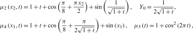
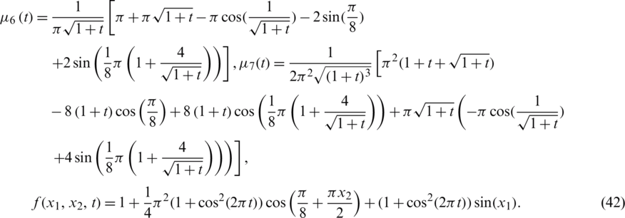
Also,

With this data, the conditions (A1)–(A6) of Theorems 1 and 2 are holds, thus the uniqueness of the solution is also ensured. The initial guesses for  and
and  , for this example has been taken as in Eq. (39).
As in Example 1, we take 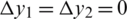 .1 and
  .025 and we first choose the case when p = 0 in the data
  ,
,  and
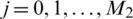
and  , in Eq. (28). The analytical Eq. (41) and numerical solutions for l(t), h(t) and a(t) is illustrated in Fig. 5, where the reconstructed timewise terms are in excellent agreement with their corresponding analytical solutions, obtaining with rmse(l) = 6.3E −3, rmse(h) = 1.7E −3 and rmse(a) = 9.8E −3, see Tab. 4.
Figure 5: The analytical Eq. (41) and numerical solutions for: (a) l(t), (b) h(t) and (c) a(t), with no noise and no regularization, for Example 2
Table 4: The values of rmse Eqs. (31) to (33), the function Eq. (27) at final iteration and the number of iterations, for 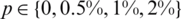 noise, for Example 2
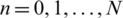
Next, we add  noise into the measured data Eqs. (12) to (14), in order to investigate the stability of the numerical results. The approximate results for the free boundaries l(t), h(t) and the thermal conductivity a(t) are illustrated in Fig. 6. From this figure it can be observed that reasonable and stable numerical results are obtained. The numerical solutions for l(t), h(t) and a(t) obtained with the
  noise have been found highly oscillatory and unstable when no regularization was employed, i.e.,
  , obtaining rmse(l) = 0.1317, rmse(h) = 0.2439 and rmse(a) = 0.2779, see Fig. 7. Therefore, regularization is required in order to restore the stability of the solution in the components l(t), h(t) and a(t). Including regularization, i.e.,
  , in Eq. (40) alleviates this instability, as shown in the regularized approximate results in Fig. 7 and Tab. 5. The absolute errors between the analytical Eq. (43) and approximate
  with the
  noise, and without and with regularization parameters, is illustrated in Fig. 8. From this figure and Tab. 5 it can be noticed that the temperature
  component is stable and accurate. Overall, the same conclusions can be carried out about the stable determination for the unknown time-dependent coefficients.
Figure 6: The analytical Eq. (41) and numerical solutions for: (a) l(t), (b) h(t) and (c) a(t), with 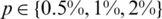 noise, for Example 2
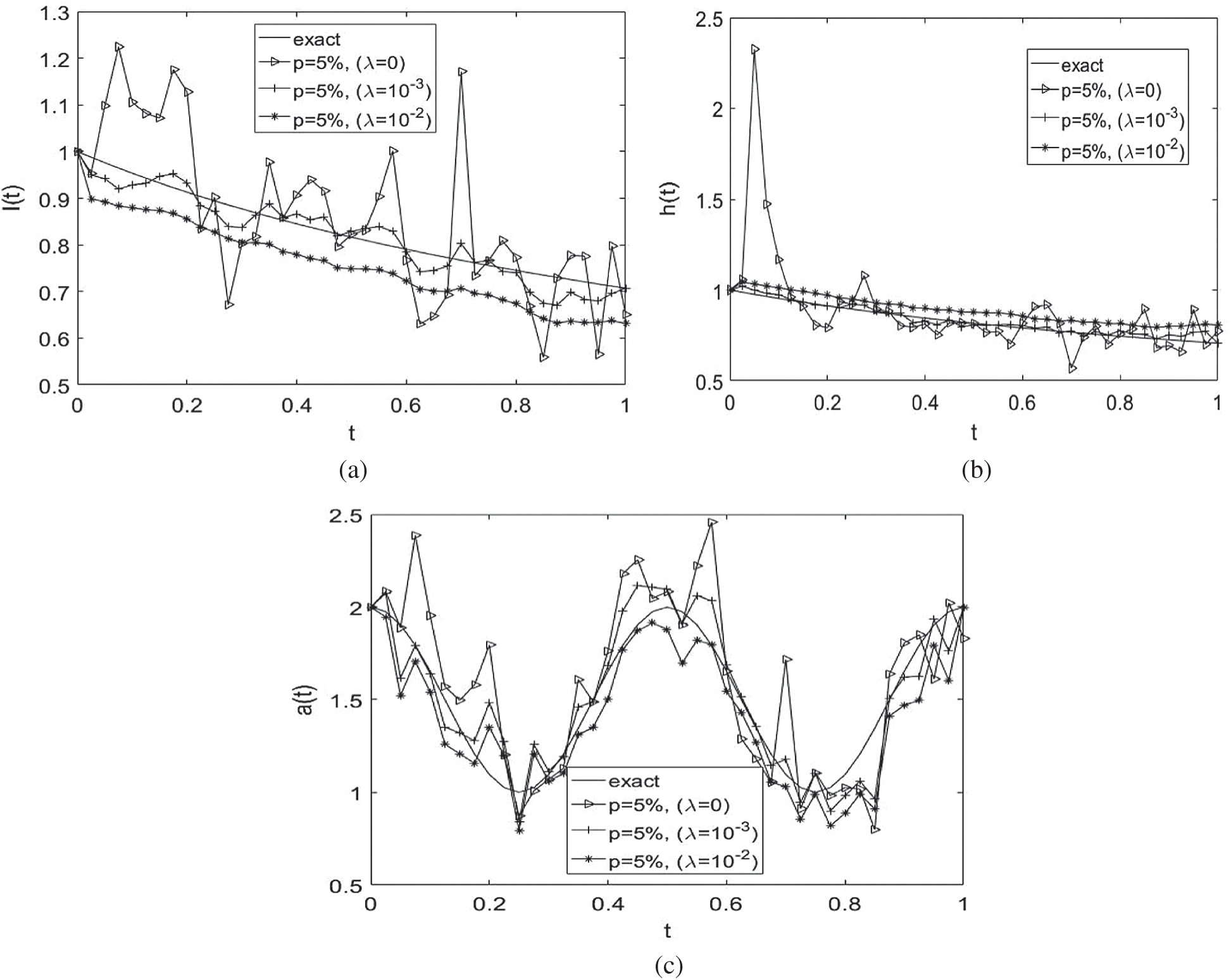
Figure 7: The analytical Eq. (41) and numerical solutions for: (a) l(t), (b) h(t) and (c) a(t), for  noise and without and with regularization, for Example 2
Table 5: The values of rmse Eqs. (31) to (33) and the number of iterations, for  noise, without and with regularization, for Example 2
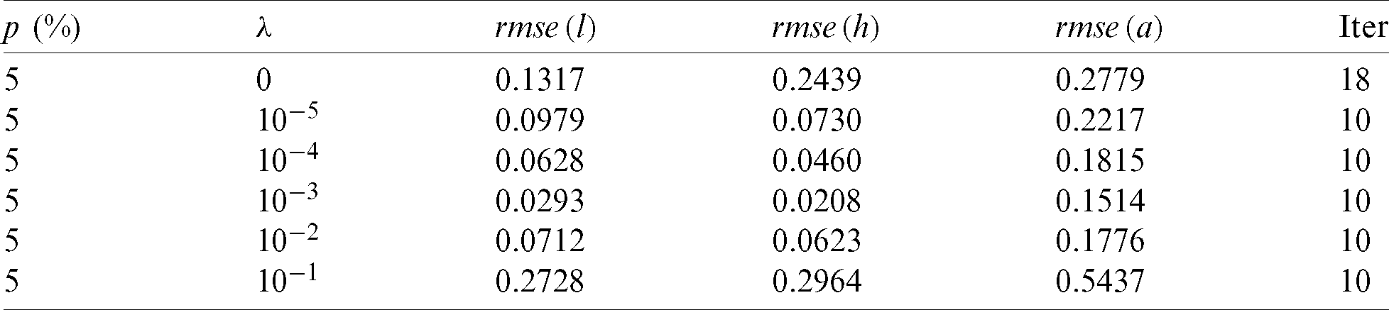
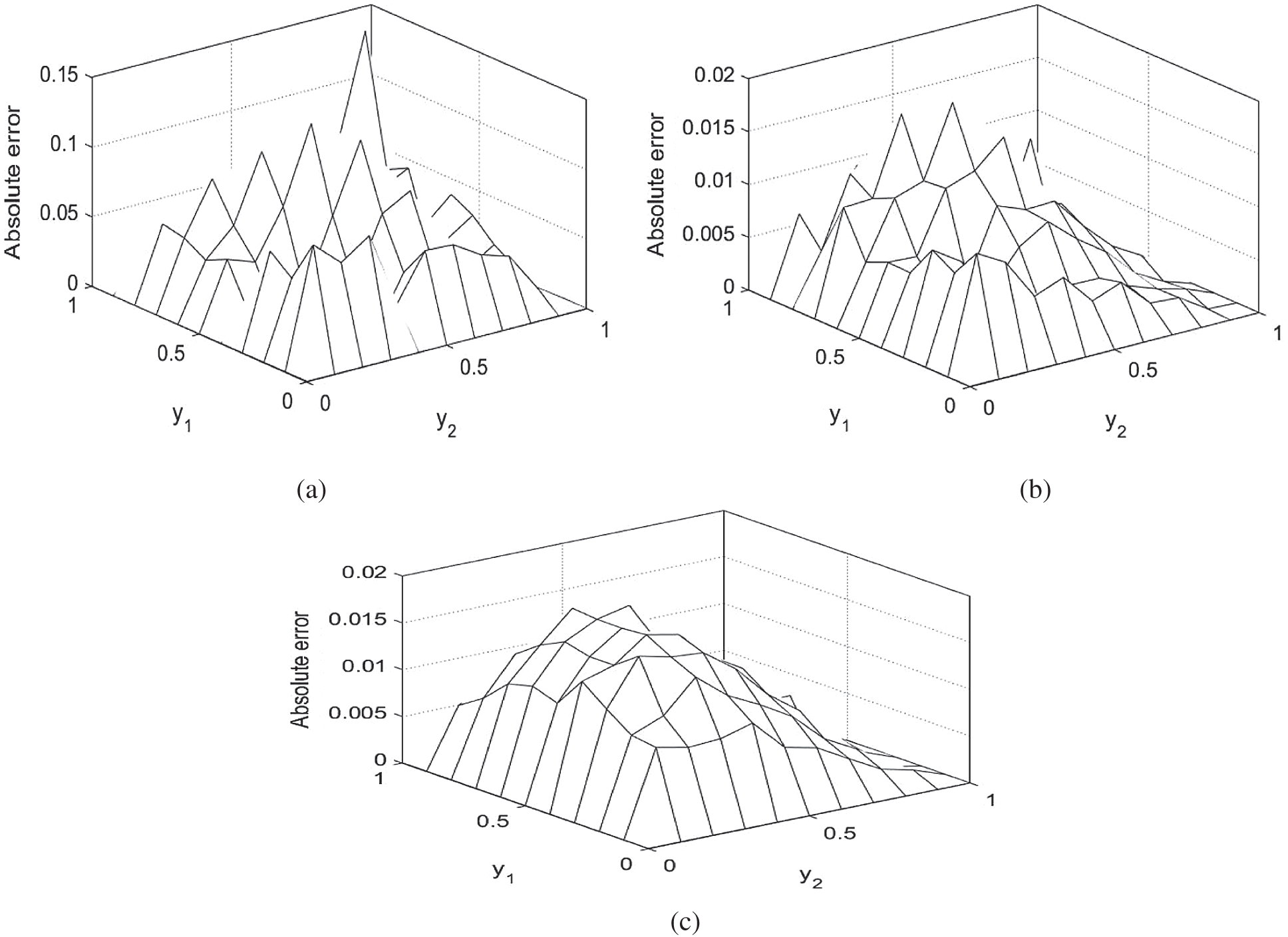
Figure 8: The absolute errors between the analytical Eq. (43) and numerical  with (a)
  , (b)
, (b)  and (c)
  , for
, for  , for Example 2
The inverse problem concerning the reconstruction of the time-dependent thermal conductivity  and free boundary coefficients l(t) and h(t) along with the temperature
  in a two-dimensional parabolic equation from the over-specification conditions has been solved for the first time numerically. The forward solver based on the ADE was employed. The inverse problem approach based on a nonlinear least-squares minimization problem using the MATLAB optimization subroutine was developed. The Tikhonov regularization has been employed in order to obtain stable and accurate solutions since the inverse problem is ill-posed. The numerical results for the inverse problem shows that stable and accurate approximate results have been obtained. Extension to three-dimensions is in principle straightforward.
Acknowledgement: The comments and suggestions made by the referees are gratefully acknowledged.
Funding Statement: The author received no specific funding for this study.
Conflicts of Interest: The authors declare that they have no conflicts of interest to report regarding the present study.
 | This work is licensed under a Creative Commons Attribution 4.0 International License, which permits unrestricted use, distribution, and reproduction in any medium, provided the original work is properly cited. |