State Estimation Moving Window Gradient Iterative Algorithm for Bilinear Systems Using the Continuous Mixed p-norm Technique

1  Introduction

Although many physical dynamic behaviors are characterized as linear systems in the neighborhood of a single operating point, when they exhibit strong nonlinearities or must be described over the entire operating range, linear models may not yield appropriate results [1–3]. Owing to that, the study of system identification and parameter estimation for nonlinear systems has drawn considerable attention of academic researchers [4–6]. Various models are exploited to describe actual nonlinear systems with relatively simple structures [7–11] such as Hammerstein systems, Bilinear systems, and Wiener systems.

The parameter estimation of the system models is important for control system analysis and design. The parameters of the models can be estimated by using some identification methods [12–15] such as the hierarchical algorithms [16–19]. In this paper, we confine our discussion to bilinear systems, which are simplicity in model structures and capable of approaching arbitrary nonlinear systems with much higher accuracy than traditional linear approximations theoretically [20]. Bruni et al. designed a bilinear time-series model-based self-tuning controller for a multi-machine power system to enhance the region of stability of the system, and return the states to their stable equilibrium [21]. Yeo et al. developed the bilinear model predictive control algorithm for paper plant systems to control the grade change operations in paper production [22]. Wang et al. simulated the bridge nonlinear boundary as bilinear translational, and applied the nonlinear least squares optimization algorithm to identify the nonlinear translational and rotational boundary parameters of the bridge [23].

Many researches have been studied in the parameter estimation of bilinear state space systems. A stochastic gradient algorithm and a gradient-based iterative algorithm have been proposed for the parameter identification of bilinear systems by using the auxiliary model. The gradient-based iterative algorithm uses fixed batch data to update the parameters, so that the parameter estimation accuracy can be greatly improved compared with the stochastic gradient algorithm. Li et al. combined the maximum likelihood theory with the data filtering technique for bilinear systems with colored noises. The state observer is vital in the field of state estimation of bilinear systems [24]. Tsai considered a H-infinity fuzzy observer for bilinear systems by means of a linear matrix inequality approach [25]. Phan et al. presented a full-order bilinear state observer for the bilinear system, which optimized the observer gain by interaction matrices [26]. Zhang et al. considered the state estimation problem of bilinear systems and proposed a state filtering method for the single-input single-output bilinear systems and multiple-input multiple-output bilinear systems by minimizing the covariance matrix of the state estimation errors [27]. Recently, some state and parameter estimation methods have been proposed for linear and bilinear state space systems in the presence of exogenous noises [28–30].

However, in industrial applications, the dynamical processes often work on various noise environments, and some works used nonlinear filtering technique such as median filtering and least mean p-norm to overcome the problems. Zayyani proposed a mixed-norm adaptive filter algorithm for systems identification based on minimization of the logarithmic continuous mixed p-norm [31]. Moreover, an improved mixed p-norm algorithm had been studied to combat non-Gaussian interference and its computational complexity as well as the mean convergence had also been analyzed [32,33].

Inspired by the above researches, we study the parameter estimation algorithms for bilinear state space models with the noise disturbances. Based on the iterative search and the state estimator, a bilinear state continues mixed p-norm gradient iteration (BSO-CMPN-GI) is proposed. The proposed algorithms control the proportions of the error norms and offer an extra degree of freedom within the adaptation. By taking into consideration each p-norm of errors for 1≤p≤2, the proposed algorithms combine the benefits of the variable error norms and thus are more robust against noise interference. Furthermore, the moving data window theory is introduced to improve the effectiveness of the proposed algorithms. The contributions of this paper are summarized as follows:

•   A state observer is designed to obtain the system states variables consisting of the product terms of state variables and control variables.

•   A bilinear state observer-based continues mixed p-norm gradient iteration (BSO-CMPN-GI) algorithm is presented for the bilinear state space system under the noise interference to estimate the unknown system parameters.

•   A bilinear state observer-based moving window CMPN-GI (BSO-MW-CMPN-GI) algorithm is derived to update collected data and thus maintain high data utilization.

The outlines of this paper are organized as follows. Section 2 introduces some definitions and proposes the identification model of the bilinear state space system and introduces a bilinear state observer for the state estimation. Sections 3 and 4 derive a BSO-CMPN-GI and a MW-CMPN-GI algorithms based on the bilinear state estimator, respectively. An example to illustrate the effectiveness of the proposed algorithms in Section 5. Finally, Section 6 gives some concluding remarks.

2  System Description and Identification Model

Consider the following single-input single-output bilinear state space modelblue:

xt+1=Axt+Bxtut+gut+wt,(1)

yt=cxt+vt,(2)

where ut∈Rn is the system input variables, yt∈Rn is the measurement output variables, xt is the state vector, wt is an uncorrelated process noise with zero mean, and vt is an uncorrelated measurement noise with zero mean. A∈Rn×n, B∈Rn×n, g∈Rn and c∈R1×n are system parameter matrix and parameter vector. Consider the observer canonical form of bilinear systems, the system parameters can be expressed as

A:=[−a110⋯0−a2010⋮⋮⋱⋮−an−10⋯01−an0⋯00]∈Rn×n,B:=[b1b2⋮bn−1bn]∈Rn×n,g:=[g1g2⋮gn−1gn]∈Rn,c:=[1,0,⋯,0,0]∈R1×n,(3)

where bj:=[bj1,bj2,…,bjn]∈R1×n,j=1,2,…,n.

Assumption 1: The dimension n of the system state vector is known, ut=0, xt=0, yt=0, wt=0 and vt=0 for t≤0.

Assumption 2: The bilinear system in Eqs. (1) and (2) is observable and controllable.

Eq. (1) can be written as

{x1,t+1=−a1x1,t+x2,t+b1xtut+g1ut+w1,t,x2,t+1=−a2x1,t+x3,t+b2xtut+g2ut+w2,t,⋮xn−1,t+1=−an−1x1,t+xn,t+bn−1xtut+gn−1ut+wn−1,t,xn,t+1=−anx1,t+bnxt+gnut++wn,t.(4)

Adding both sides of the above equations has

x1,t+1=−a1x1,t−a2x1,t−1−⋯−anxt−n+1+b1xtut+b2xt−1ut−1+⋯+bnxt−n+1ut−n+1+g1ut+g2ut−1+⋯+gnut−n+1+w1£s¬t+w2,t−1+⋯+wn,t−n+1=−∑j=1najx1,t−j+1+∑j=1nbjxt−j+1ut−j+1+∑j=1ngjut−j+1+∑j=1nwj,t−j+1.(5)

Substituting Eq. (5) into Eq. (2) obtains the regression form of the bilinear state model

yt=−∑j=1najx1,t−j+∑j=1nbjxt−jut−j+∑j=1ngjut−j+∑j=1nwj,t−j+vt.(6)

Define the information vector ψt and parameter vector ϑ as

ψt:=[dt,kt,ht]T∈Rn2+2n,(7)

dt:=[−x1,t−1,−x1,t−2,…,−x1,t−n]T∈Rn,(8)

kt:=[xt−1Tut−1,xt−2Tut−2,…,xt−nTut−n]T∈Rn2,(9)

ht:=[ut−1,ut−2,…,ut−n]T∈Rn,(10)

ϑ:=[a,B,g]T∈Rn2+2n,(11)

a:=[a1,a2,…,an]T∈Rn,(12)

B:=[b1,b2,…,bn]T∈Rn2,(13)

g:=[g1,g2,…,gn]T∈Rn.(14)

Redefine the noise term as

et:=∑j=1nwj,t−j+vt.(15)

Eq. (6) can be rewritten as

yt=ψtTϑ+et.(16)

The proposed parameter estimation algorithms in this paper are based on this identification model in (16). Many identification methods are derived based on the identification models of the systems [34–43] and these methods can be used to estimate the parameters of other linear systems and nonlinear systems [44–50] and can be applied to other fields such as chemical process control systems. The purpose of this paper is to obtain the estimates of the unknown parameters in the bilinear state space model by means of the measurement data {ut,yt}. However, the state space model contains not only unknown parameters, but also unknown state variables. That means the information vector ψt in Eq. (16) contains the unknown state vector xt−i. Given this, we adopt the state observer for estimating the unknown states variables [51]. According to the bilinear state space model, the state observer is designed as

x^t+1=A^x^t+B^x^tut+g^ut,(17)

where

A^=[−a^110⋯0−a^2010⋮⋮⋱⋮−a^n−10⋯01−a^n0⋯00]∈Rn×n,B^=[b^1b^2⋮b^n−1b^n]∈Rn×n,g^=[g^1g^2⋮g^n−1g^n]∈Rn.

Remark 1: Differently from the identification of bilinear-in-parameter systems which involve the product terms of the parameter vectors and the information matrices, this paper studies the identification problem of bilinear state-space systems with the product terms of state variables and control variables, which makes it difficult for the parameter and state estimation.

3  Bilinear State Observer Based Continuous Mixed p-norm Gradient Iterative Identification Algorithm

Set the data length be L, based on the input and output data {ut,yt,1⩽t⩽L}, define the stacked input vector YL and the stacked information matrix ΨL as

YL:=[yLyL−1⋮yt⋮y1]∈RL,ΨL:=[ψLTψL−1T⋮ψtT⋮ψ1T]∈RL×(n2+2n).

To suppress the effect of noise interference, define the continuous mixed p-norm cost function

J1(ϑ):=∫12λ(p)|VL|pdp,(18)

where λ(p) is the probability density-like weighting function which is constrained by ∫12λt(p)dp=1, and VL:=YL−ΨLϑ.

Using the negative gradient search method to minimize the cost function J1(ϑ) with respect to ϑ gives

grad[J1(ϑ)]=∂J1(ϑ)∂ϑ=[∂J1(ϑ)∂a∂J1(ϑ)∂B∂J1(ϑ)∂g](19)

where

∂J1(ϑ)∂a=∫12pλ(p)|VL|p−1sgn(VL)∂(VL)∂adp=−∫12pλ(p)|VL|p−1sgn(VL)dp[dL,dL−1,…,dt,…,d1]T,∂J1(ϑ)∂B=−∫12pλ(p)|VL|p−1sgn(VL)dp[kL,kL−1,…,kt,…,k1]T,∂J1(ϑ)∂g=−∫12pλ(p)|VL|p−1sgn(VL)dp[hL,hL−1,…,ht,…,h1]T.

Therefore, Eq. (19) can be expressed as

grad[J1(ϑ)]=−∫12pλ(p)|VL|p−1sgn(VL)ΨLdp=−ΓLsgn(VL)ΨL,

where

ΓL=∫12pλ(p)|VL|p−1dp.(20)

Let s=1,2,3,… be the iteration variables, ϑ^s be the parameter estimation vector at iteration s. Using the negative gradient search and minimizing J1(ϑ) yield

ϑ^s=ϑ^s−1−μsgrad[J1(ϑ^s−1)]=ϑ^s−1+μsΓLsgn(VL)ΨL,(21)

where μs is the iteration step size [52–57], which satisfies

0<μs⩽2λmax[ΨLTΨL].(22)

Eqs. (21) and (22) cannot figure out the parameter estimation vector ϑ^s, because the information matrix ΨL contains the unknown states xt−j. The solution is to replace the unknown states xt−j in the information matrix with their estimates obtained by the state observer at the previous iteration. Define the estimated information matrix as

Ψ^Ls:=[(ψ^Ls)T,(ψ^L−1s)T,…,(ψ^ts)T,…,(ψ^1s)T]T∈RL×(n2+2n),ψ^ts=[−x^1,t−1s−1,…,−x^1,t−ns−1,(x^t−1s−1)Tut−1,…,(x^t−ns−1)Tut−n,ut−1,…,ut−n]T∈Rn2+2n,

where x^t−js−1 is given by

x^t−js−1=A^s−1x^t−j−1s−1+B^s−1x^t−j−1s−1ut−j−1+g^s−1ut−j−1,j=1,2,…,L.

Replace the information matrix ΨL in Eqs. (21) and (22) with its estimated value Ψ^L, the estimate V^Ls at iteration s is YL−Ψ^Lsϑ^s−1. Replacing VLs in (20) with its estimates gives

Γ^Ls=∫12pλ(p)|V^Ls|p−1dp.(23)

To obtain a closed form formula for Γ^Ls, a uniform weighting function λ(p)=1 is assumed. Then, the bilinear state observe-based continuous mixed p-norm gradient iterative (BSO-CMPN-GI) identification algorithm (24)–(30) for the bilinear system is summarized in the following:

ϑ^s=ϑ^s−1+μsΓ^Lssgn(V^Ls)Ψ^Ls,(24)

0<μs⩽2λmax[(Ψ^Ls)TΨ^Ls],(25)

Γ^Ls=(2|V^Ls|−1)ln⁡(|V^Ls|)−|V^Ls|+1ln2(|V^Ls|),(26)

V^Ls=YL−Ψ^Lsϑ^s−1,(27)

Ψ^Ls=[(ψ^Ls)T,(ψ^L−1s)T,…,(ψ^ts)T,…,(ψ^1s)T]T,(28)

ψ^ts=[−x^1,t−1s−1,…,−x^1,t−ns−1,(x^t−1s−1)Tut−1,…,(x^t−ns−1)Tut−n,ut−1,…,ut−n]T,(29)

x^t−js=A^sx^t−j−1s+B^sx^t−j−1sut−j−1+g^sut−j−1.(30)

The flowchart of the BSO-CMPN-GI algorithm in Eqs. (24)–(30) is shown in Fig. 1.

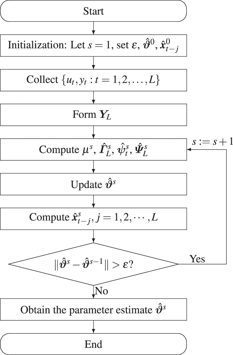
Figure 1: The flowchart of the BSO-CMPN-GI algorithm

Remark 2: The parameter p in BSO-CMPN-GI is adapted by continuous p-norm without resorting to a priori knowledge of the noise.

Remark 3: The BSO-CMPN-GI algorithm makes full use of the measurement data in each iteration of the calculation process, but it requires a batch of data to be collected in advance, and thus is implemented offline. Therefore, an on-line identification algorithm derived from the BSO-CMPN-GI algorithm will be introduced by exploiting the past and current measurement data to estimate the unknown parameters in Section 4.

4  Bilinear State Observe Moving Window Continuous Mixed p-norm Gradient Iterative Algorithm

In this section, we introduce the moving window method to derive an on-line identification algorithm and enhance the performance of the BSO-CMPN-GI algorithm. The length of the moving window is set as a fixed value m. Define the stacked output vector Yt,m and the stacked information matrix Ψt,m as

Yt,m:=[ytyt−1⋮yt−m+1]∈Rh,Ψt,m:=[ψtTψt−1T⋮ψt−m+1T]∈Rh×(n2+2n).

Consider the measurements from t−m+1 to t and define the cost function

J2(ϑ):=∫12λt(p)|Vt,m|pdp,(31)

where

Vt,m=Yt,m−Ψt,mϑ(32)

=[etet−1⋮et−m+1]=[yt−dtTa−ktTB−htTgyt−1−dt−1Ta−kt−1TB−ht−1Tg⋮yt−m+1−dt−m+1Ta−kt−m+1TB−ht−m+1Tg],(33)

Taking the gradient of J2(ϑ) gives

grad[J2(ϑ)]=∂J2(ϑ)∂ϑ=[∂J2(ϑ)∂a∂J2(ϑ)∂B∂J2(ϑ)∂g],(34)

where

∂J2(ϑ)∂a=∫12pλt(p)|Vt,m|p−1sgn(Vt,m)∂(Vt,m)∂adp=−∫12pλt(p)|Vt,m|p−1sgn(Vt,m)dp[dt,dt−1,dt−m+1]T,∂J2(ϑ)∂B=−∫12pλt(p)|Vt,m|p−1sgn(Vt,m)dp[kt,kt−1,…,kt−m+1]T,∂J2(ϑ)∂g=−∫12pλt(p)|Vt,m|p−1sgn(Vt,m)dp[ht,ht−1,…,ht−m+1]T.

Therefore, Eq. (4) can be expressed as

grad[J2(ϑ)]=−∫12pλt(p)|Vt,m|p−1sgn(Vt,m)Ψt,mdp=−Γt,msgn(Vt,m)Ψt,m,

where

Γt,m=∫12p|Vt,m|p−1dp.(35)

Let s=1,2,3,… be iteration variables. Similar to the derivation of the BSO-CMPN-GI algorithm, using the negative gradient search method and minimizing J2(ϑ) get

ϑ^ts=ϑ^ts−1−μtsgrad[J2(ϑ^ts−1)]=ϑ^ts−1+μtsΓt,msgn(Vt,m)Ψt,m,(36)

where

0<μts⩽2λmax[Ψt,mTΨt,m].(37)

As pointed earlier in Section 3, the unknown states xt−j in the information matrix Ψt,m are replaced with their estimates. The estimated information matrix Ψ^t,ms is redefined as

Ψ^t,ms:=[(ψ^ts)T,(ψ^t−1s)T,…,(ψ^t−m+1s)T]∈RL×(n2+2n)ψ^ts=[−x^1,t−1s−1,…,−x^1,t−ns−1,(x^t−1s−1)Tut−1,…,(x^t−ns−1)Tut−n,ut−1,…,ut−n]T∈R(n2+2n).

where xt−js−1 is estimated by the state observer:

x^t−js−1=A^ts−1x^t−j−1s−1+B^ts−1x^t−j−1s−1ut−j−1+g^ts−1ut−j−1.(38)

Based on the above derivation, a bilinear state observe-based moving window continuous mixed p-norm gradient iterative (BSO-MW-CMPN-GI) algorithm proposed for the bilinear state space system is summarized as follows:

ϑ^ts=ϑ^ts−1+μtsΓt,mssgn(Vt,ms)Ψ^t,ms,(39)

0<μts⩽2λmax[(Ψ^t,ms)TΨ^t,ms],(40)

Γ^t,ms=(2|V^t,ms|−1)ln⁡(|V^t,ms|)−|V^t,ms|+1ln2(|V^t,ms|),(41)

V^t,ms=Yt,m−Ψ^t,msϑ^ts−1,(42)

Ψ^t,ms:=[(ψ^ts)T,(ψ^t−1s)T,…,(ψ^t−m+1s)T],(43)

ψ^ts=[−x^1,t−1s−1,…,−x^1,t−ns−1,(x^t−1s−1)Tut−1,…,(x^t−ns−1)Tut−n,ut−1,…,ut−n]T,(44)

x^t−js=A^tsx^t−j−1s+B^tsx^t−j−1sut−j−1+g^tsut−j−1.(45)

The flowchart of the BSO-MW-CMPN-GI algorithm in Eqs. (39)–(45) is shown in Fig. 2.

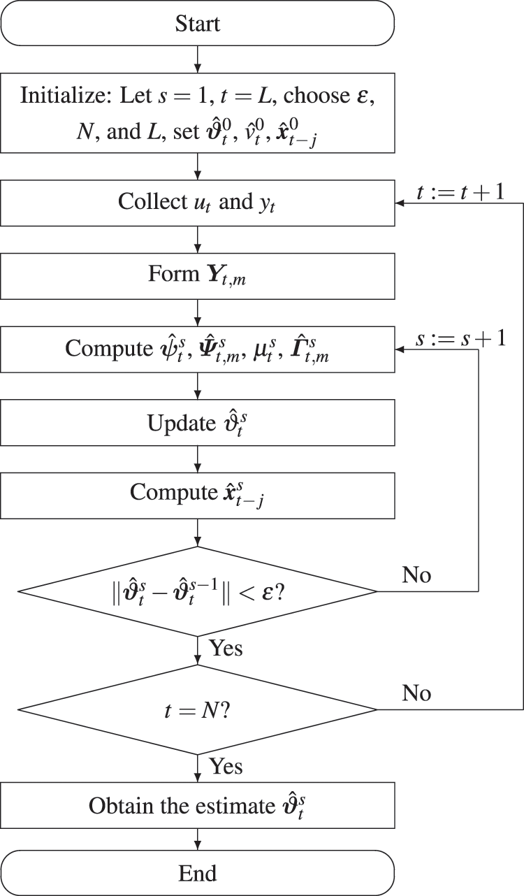
Figure 2: The flowchart of the BSO-MW-CMPN-GI algorithm for computing ϑ^ts

Remark 4: The parameter estimate given by the BSO-MW-CMPN-GI algorithm depends only on the iterative counter s, but also time t. As the sampling time t increases, the BSO-MW-CMPN-GI algorithm can utilize a batch of data to calculate the parameter estimate simultaneously.

5  Simulation

Case 1: About parameter estimation

Consider a second-order bilinear state space system:

xt+1=[−0.801−0.450]xt+[0.040.150.250.18]xtut+[1.271.16]ut+wt,yt=[1,0]xt+vt.

The parameter vector to be estimated is

ϑ=[0.80,0.45,0.04,0.15,0.25,0.18,1.27,1.16]T

In simulation, the input {ut} is taken as an uncorrelated uniform disturbance random signal sequence with zero mean and unit variance, {wt} is taken as an uncorrelated process white noise vector sequence with zero mean and variance Q=[σw2,0;0,σw2], σw2=0.022, {vt} is taken as a white noise vector sequence with zero mean and variance σv2=1.002 and σv2=1.502, respectively. Apply the BSO-CMPN-GI algorithm in Eqs. (24)–(30) and the BSO-MW-CMPN-GI algorithm in Eqs. (39)–(45) with the data length L=500 to estimate the states xt and parameters ϑ of this bilinear system, respectively. For comparison with the different algorithm, we introduce the bilinear state observe-based gradient iterative (BSO-GI) algorithm. In the BSO-MW-CMPN-GI algorithm, s=15 represents the iteration variable, and m=60 represents the recursive variable. The parameter estimates and errors δ:=‖ϑ^t−ϑ‖/‖ϑ‖ vs. s of the BSO-GI algorithm, the BSO-CMPN-GI algorithm and the BSO-MW-CMPN-GI algorithm with different noise variances are shown in Tables 1 and 2. The parameter estimation errors δ vs. s of the BSO-GI algorithm, the BSO-CMPN-GI algorithm and the BSO-MW-CMPN-GI algorithm with different noise variances are shown in Figs. 3–6, respectively. The estimated output (EO) and the actual output (AO) of the four algorithms are shown in Figs. 7 and 8. From Tables 1 and 2 and Figs. 3–8, the following conclusions can be drawn:

•   The parameter estimation errors given by the BSO-GI algorithm, the BSO-CMPN-GI algorithm and the BSO-MW-CMPN-GI algorithm become smaller as the iteration s increases. It thus to say the proposed algorithms are effective for bilinear systems.

•   The state estimates are close to their true values with t increasing.

•   Under the same data length, a lower noise variance leads to higher parameter estimation accuracy by the BSO-GI algorithm, the BSO-CMPN-GI algorithm and the BSO-MW-CMPN-GI algorithm.

•   The BSO-CMPN-GI algorithm and the BSO-MW-CMPN-GI algorithm possess higher parameter estimation accuracy at the same noise variance compared with the BSO-GI algorithm.

•   When comparing the BSO-CMPN-GI algorithm and the BSO-MW-CMPN-GI algorithm, the parameter estimation errors of the BSO-MW-CMPN-GI algorithm become smaller with m increasing, and approach to zero if m is large enough.

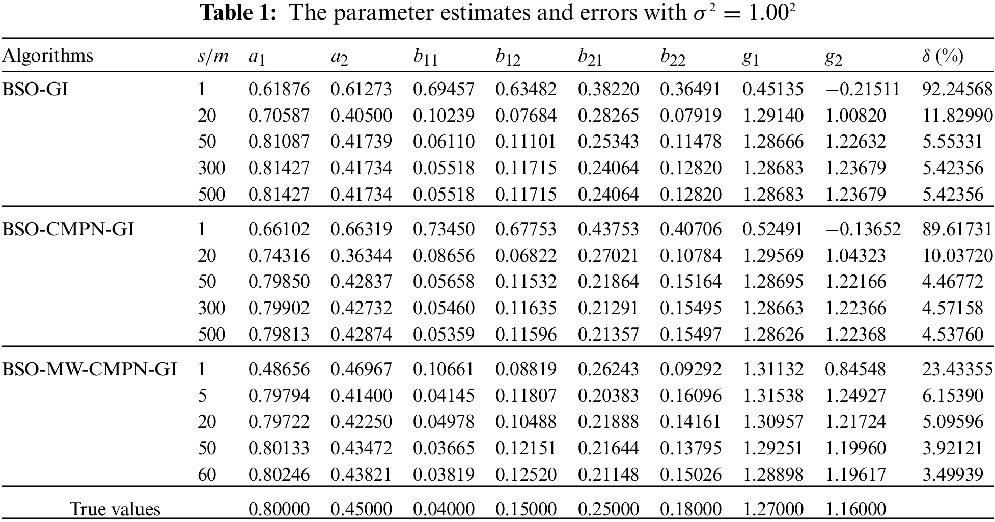
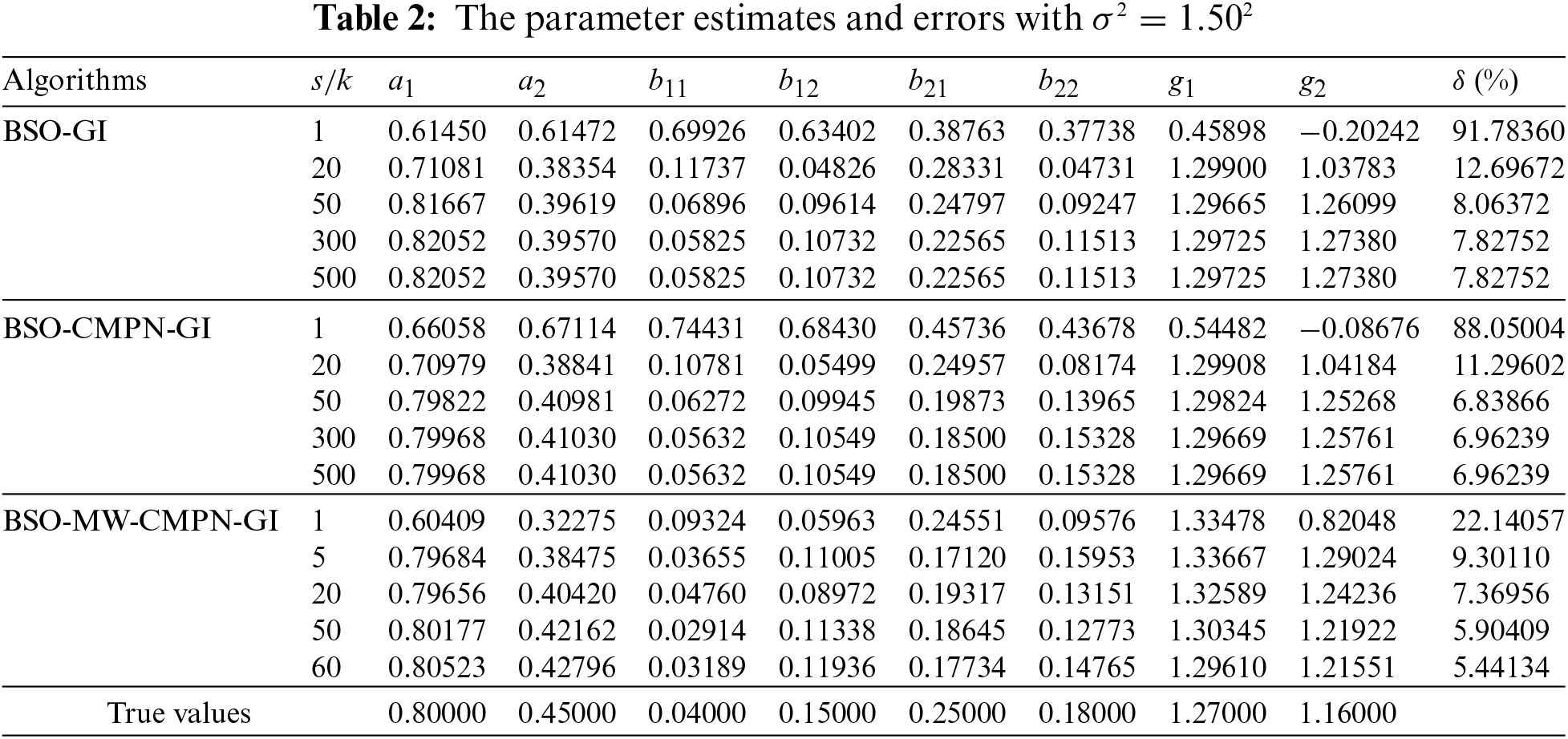
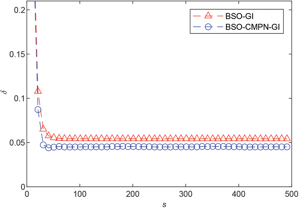
Figure 3: The estimation errors δ vs. t with σ2=1.002

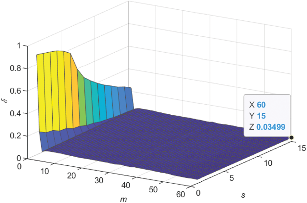
Figure 4: The BSO-MW-CMPN-GI estimation errors δ vs. m and s (m=60 and s=15) with σ2=1.002

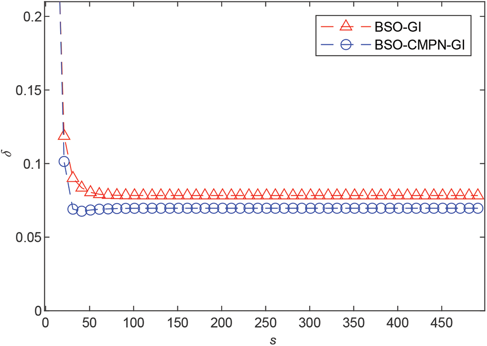
Figure 5: The estimation errors δ vs. t with σ2=1.502

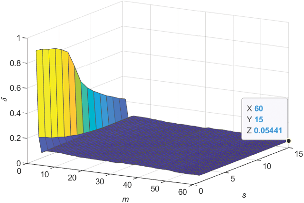
Figure 6: The BSO-MW-CMPN-GI estimation errors δ vs. m and s (m=60 and s=15) with σ2=1.502

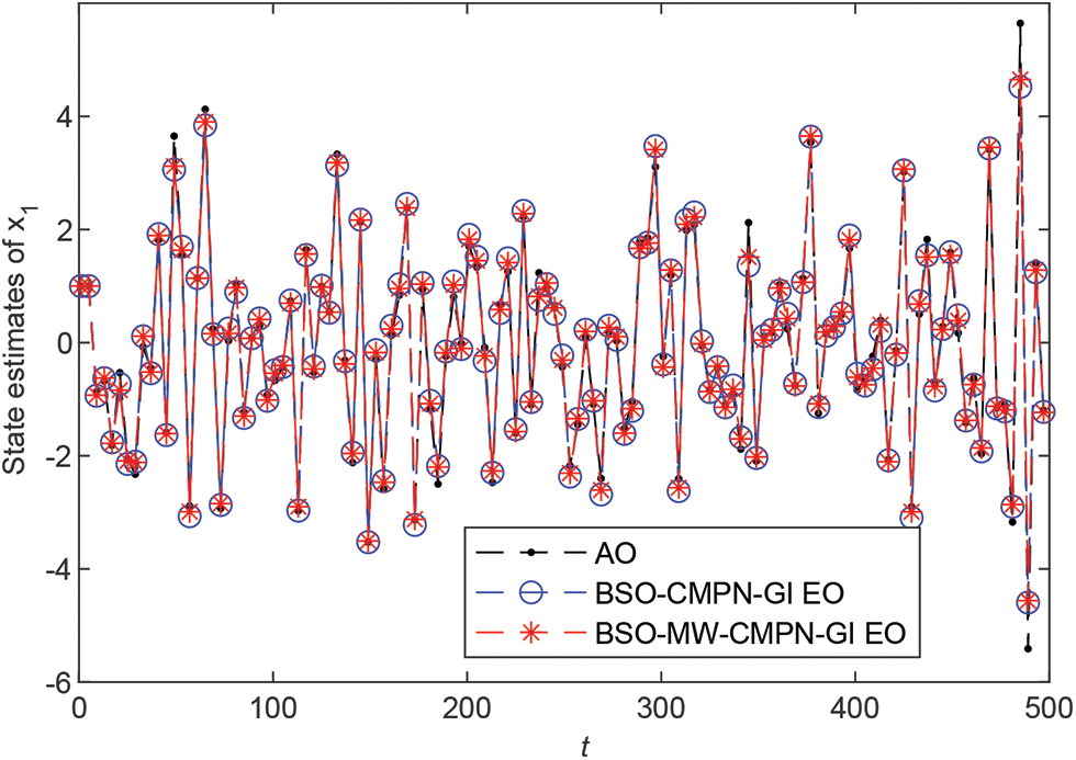
Figure 7: State x1,t and the estimated state x^1,t vs. t

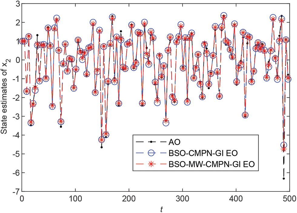
Figure 8: State x2,t and the estimated state x^2,t vs. t

Case 2: About model validation

Applying the BSO-CMPN-GI algorithm and the BSO-MW-CMPN-GI algorithm to construct the estimated model for the model validation, respectively. Take the data from t=1001 to t=2000 to calculate the root mean square errors (RMSEs) of the predicted output y^t. Using the BSO-CMPN-GI and BSO-MW-CMPN-GI estimates in Table 1 with the noise variance σv2=1.002. The actual output (AO) yt and the predicted output (PO) y^t are plotted in Fig. 9. The RMSEs of the BSO-GI, BSO-CMPN-GI and BSO-MW-CMPN-GI are

δ1=1Lt∑j=10012000[yj−y^BSO−GIj]2=1.0223,δ2=1Lt∑j=10012000[yj−y^BSO−CMPN−GIj]2=1.0187,δ3=1Lt∑j=10012000[yj−y^BSO−MW−CMPN−GIj]2=1.0127,

where y^BSO - GIj, y^BSO - CMPN - GIj and y^BSO - MW - CMPN - GIj represent the predicted output of the BSO-GI algorithm, the BSO-CMPN-GI algorithm and the BSO-MW-CMPN-GI algorithm, respectively.

From Fig. 9, we can see that the predicted outputs of the BSO-CMPN-GI and the BSO-MW-CMPN-GI are very close to the true outputs, and the RMSEs of the two algorithms are very close to the noise standard deviation σv2=1.002. In other words, the estimated model can capture the dynamics of the system.

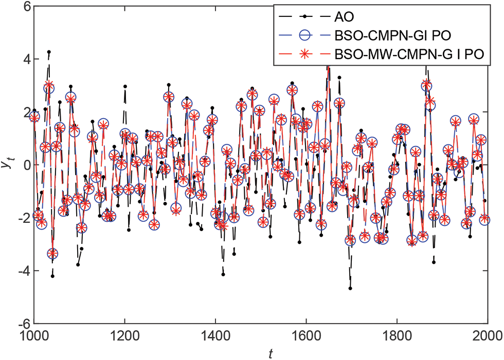
Figure 9: The system actual outputs and the predicted outputs vs. t with σv2=1.002

6  Conclusions

This paper studies the parameter identification problems of the nonlinear systems described by the bilinear state space models with the noise disturbances. A bilinear state observe-based continuous mixed p-norm gradient iterative algorithm and a bilinear state observe-based moving window continuous mixed p-norm gradient iterative algorithm are proposed to estimate the parameters of the bilinear system. The proposed optimal algorithms are robustness for stochastic white noise by means of the continuously mixed p-norms theory. In order to improve the performance of the proposed algorithms, the moving window identification theory is introduced into the proposed algorithm. Although the proposed algorithms are effective for identifying the bilinear system, it also has some limitations. For example, the disturbance noise is confined to the white noise. The proposed model parameter estimation methods in the paper can combine some mathematical strategies [58–60] and other estimation algorithms [61–65] to study the parameter identification problems of linear and nonlinear systems with different disturbances [66–68] and can be applied to other fields [69–74] such as engineering application systems.

Funding Statement: This research was funded by the National Natural Science Foundation of China (No. 61773182) and the 111 Project (B12018).

Conflicts of Interest: The authors declare that they have no conflicts of interest to report regarding the present study.

References

1. Xu, L. (2022). Separable multi-innovation newton iterative modeling algorithm for multi-frequency signals based on the sliding measurement window. Circuits Systems and Signal Processing, 41(2), 805–830. DOI 10.1007/s00034-021-01801-x. [Google Scholar] [CrossRef]
2. Xu, L. (2022). Separable newton recursive estimation method through system responses based on dynamically discrete measurements with increasing data length. International Journal of Control Automation and Systems, 20(2), 432–443. DOI 10.1007/s12555-020-0619-y. [Google Scholar] [CrossRef]
3. Zhang, X., Liu, Q., Hayat, T. (2020). Recursive identification of bilinear time-delay systems through the redundant rule. Journal of the Franklin Institute, 357(1), 726–747. DOI 10.1016/j.jfranklin.2019.11.003. [Google Scholar] [CrossRef]
4. Gan, M., Chen, G., Chen, L., Chen, C. (2020). Term selection for a class of separable nonlinear models. IEEE Transactions on Neural Networks and Learning Systems, 31(2), 445–451. DOI 10.1109/TNNLS.5962385. [Google Scholar] [CrossRef]
5. Ding, F. (2013). Coupled-least-squares identification for multivariable systems. IET Control Theory and Applications, 7(1), 68–79. DOI 10.1049/iet-cta.2012.0171. [Google Scholar] [CrossRef]
6. Ding, F., Liu, X. G., Chu, J. (2013). Gradient-based and least-squares-based iterative algorithms for hammerstein systems using the hierarchical identification principle. IET Control Theory and Applications, 7(2), 176–184. DOI 10.1049/iet-cta.2012.0313. [Google Scholar] [CrossRef]
7. Zhao, Y. B., Liu, G. P., Rees, D. (2008). A predictive control-based approach to networked hammerstein systems: Design and stability analysis. IEEE Transactions on Cybernetics, 38(3), 700–708. DOI 10.1109/TSMCB.2008.918572. [Google Scholar] [CrossRef]
8. Mahata, K., Schoukens, J., de Cock, A. (2016). Information matrix and D-optimal design with Gaussian inputs for wiener model identification. Automatica, 69, 65–77. DOI 10.1016/j.automatica.2016.02.026. [Google Scholar] [CrossRef]
9. Wang, Y. J., Tang, S. H., Gu, X. B. (2022). Parameter estimation for nonlinear volterra systems by using the multi-innovation identification theory and tensor decomposition. Journal of the Franklin Institute, 359(2), 1782–1802. DOI 10.1016/j.jfranklin.2021.11.015. [Google Scholar] [CrossRef]
10. Xu, L., Song, G. L. (2020). A recursive parameter estimation algorithm for modeling signals with multi-frequencies. Circuits Systems and Signal Processing, 39(8), 4198–4224. DOI 10.1007/s00034-020-01356-3. [Google Scholar] [CrossRef]
11. Wang, Y. J., Yang, L. (2021). An efficient recursive identification algorithm for multilinear systems based on tensor decomposition. International Journal of Robust and Nonlinear Control, 31(11), 7920–7936. DOI 10.1002/rnc.5718. [Google Scholar] [CrossRef]
12. Ding, F., Zhang, X., Xu, L. (2019). The innovation algorithms for multivariable state-space models. International Journal of Adaptive Control and Signal Processing, 33(11), 1601–1608. DOI 10.1002/acs.3053. [Google Scholar] [CrossRef]
13. Ding, F., Liu, G., Liu, X. P. (2011). Parameter estimation with scarce measurements. Automatica, 47(11), 1646–1655. DOI 10.1016/j.automatica.2011.05.007. [Google Scholar] [CrossRef]
14. Liu, Y. J., Shi, Y. (2014). An efficient hierarchical identification method for general dual-rate sampled-data systems. Automatica, 50(3), 962–970. DOI 10.1016/j.automatica.2013.12.025. [Google Scholar] [CrossRef]
15. Zhang, X. (2022). Optimal adaptive filtering algorithm by using the fractional-order derivative. IEEE Signal Processing Letters, 29, 399–403. DOI 10.1109/LSP.2021.3136504. [Google Scholar] [CrossRef]
16. Ding, J., Liu, X. P., Liu, G. (2011). Hierarchical least squares identification for linear SISO systems with dual-rate sampled-data. IEEE Transactions on Automatic Control, 56(11), 2677–2683. DOI 10.1109/TAC.2011.2158137. [Google Scholar] [CrossRef]
17. Ding, F., Liu, Y. J., Bao, B. (2012). Gradient based and least squares based iterative estimation algorithms for multi-input multi-output systems. Proceedings of the Institution of Mechanical Engineers, Part I: Journal of Systems and Control Engineering, 226(1), 43–55. DOI 10.1177/0959651811409491. [Google Scholar] [CrossRef]
18. Xu, L., Chen, F. Y., Hayat, T. (2021). Hierarchical recursive signal modeling for multi-frequency signals based on discrete measured data. International Journal of Adaptive Control and Signal Processing, 35(5), 676–693. DOI 10.1002/acs.3221. [Google Scholar] [CrossRef]
19. Wang, Y. J. (2016). Novel data filtering based parameter identification for multiple-input multiple-output systems using the auxiliary model. Automatica, 71, 308–313. DOI 10.1016/j.automatica.2016.05.024. [Google Scholar] [CrossRef]
20. Mohler, R. R., Kolodziej, W. J. (2007). An overview of bilinear system theory and applications. IEEE Transactions on Systems Man and Cybernetics, 10(10), 683–688. DOI 10.1109/TSMC.1980.4308378. [Google Scholar] [CrossRef]
21. Bruni, C., Dipillo, G., Koch, G. (2003). Bilinear systems: An appealing class of “nearly linear” systems in theory and applications. IEEE Transactions on Automatic Control, 19(4), 334–348. DOI 10.1109/TAC.1974.1100617. [Google Scholar] [CrossRef]
22. Yeo, Y. K., Choo, Y. U. (2006). Bilinear model predictive control of grade change operations in paper production plants. Korean Journal of Chemical Engineering, 23(2), 167–170. DOI 10.1007/BF02705710. [Google Scholar] [CrossRef]
23. Wang, Z. C., Zha, G. P., Ren, W. X. (2018). Nonlinear boundary parameter identification of bridges based on temperature-induced strains. Structural Engineering and Mechanics, 68(5), 563–573. DOI 10.12989/sem.2018.68.5.563. [Google Scholar] [CrossRef]
24. Li, M., Liu, X. (2020). Maximum likelihood least squares based iterative estimation for a class of bilinear systems using the data filtering technique. International Journal of Control Automation and Systems, 18(6), 1581–1592. DOI 10.1007/s12555-019-0191-5. [Google Scholar] [CrossRef]
25. Tsai, S. H. (2012). A global exponential fuzzy observer design for time-delay takagi-sugeno uncertain discrete fuzzy bilinear systems with disturbance. IEEE Transactions on Fuzzy Systems, 20(6), 1063–1075. DOI 10.1109/TFUZZ.2012.2192936. [Google Scholar] [CrossRef]
26. Phan, M. Q., Vicario, F., Longman, R. W., Betti, R. (2015). Optimal bilinear observers for bilinear state-space models by interaction matrices. International Journal of Control, 88(8), 1504–1522. DOI 10.1080/00207179.2015.1007530. [Google Scholar] [CrossRef]
27. Zhang, X., Yang, E. (2019). State estimation for bilinear systems through minimizing the covariance matrix of the state estimation errors. International Journal of Adaptive Control and Signal Processing, 33(7), 1157–1173. DOI 10.1002/acs.3027. [Google Scholar] [CrossRef]
28. Zhang, X. (2020). Adaptive parameter estimation for a general dynamical system with unknown states. International Journal of Robust and Nonlinear Control, 30(4), 1351–1372. DOI 10.1002/rnc.4819. [Google Scholar] [CrossRef]
29. Zhang, X. (2020). Recursive parameter estimation methods and convergence analysis for a special class of nonlinear systems. International Journal of Robust and Nonlinear Control, 30(4), 1373–1393. DOI 10.1002/rnc.4824. [Google Scholar] [CrossRef]
30. Zhang, X. (2020). Recursive parameter estimation and its convergence for bilinear systems. IET Control Theory and Applications, 14(5), 677–688. DOI 10.1049/iet-cta.2019.0413. [Google Scholar] [CrossRef]
31. Zayyani, H. (2014). Continuous mixed p-norm adaptive algorithm for system identification. IEEE Signal Process Letters, 21(9), 1108–1110. DOI 10.1109/LSP.2014.2325495. [Google Scholar] [CrossRef]
32. Shi, L., Zhao, H., Zakharov, Y. (2019). Generalized variable step size continuous mixed
33. Shi, L., Zhao, H. (2021). Generalized variable step-size diffusion continuous mixed
34. Ding, F., Chen, T. (2004). Combined parameter and output estimation of dual-rate systems using an auxiliary model. Automatica, 40(9), 1739–1748. DOI 10.1016/j.automatica.2004.05.001. [Google Scholar] [CrossRef]
35. Ding, F., Chen, T. (2005). Parameter estimation of dual-rate stochastic systems by using an output error method. IEEE Transactions on Automatic Control, 50(9), 1436–1441. DOI 10.1109/TAC.2005.854654. [Google Scholar] [CrossRef]
36. Ding, F., Shi, Y., Chen, T. (2017). Auxiliary model-based least-squares identification methods for hammerstein output-error systems. Systems & Control Letters, 56(7), 373–380. DOI 10.1016/j.sysconle.2006.10.026. [Google Scholar] [CrossRef]
37. Ji, Y., Kang, Z., Zhang, C. (2021). Two-stage gradient-based recursive estimation for nonlinear models by using the data filtering. International Journal of Control Automation and Systems, 19(8), 2706–2715. DOI 10.1007/s12555-019-1060-y. [Google Scholar] [CrossRef]
38. Wang, J. W., Ji, Y., Zhang, C. (2021). Iterative parameter and order identification for fractional-order nonlinear finite impulse response systems using the key term separation. International Journal of Adaptive Control and Signal Processing, 35(8), 1562–1577. DOI 10.1002/acs.3257. [Google Scholar] [CrossRef]
39. Li, M. H., Liu, X. M. (2021). Iterative identification methods for a class of bilinear systems by using the particle filtering technique. International Journal of Adaptive Control and Signal Processing, 35(10), 2056–2074. DOI 10.1002/acs.3308. [Google Scholar] [CrossRef]
40. Zhou, Y. H. (2020). Modeling nonlinear processes using the radial basis function-based state-dependent autoregressive models. IEEE Signal Processing Letters, 27, 1600–1604. DOI 10.1109/LSP.2020.3021925. [Google Scholar] [CrossRef]
41. Zhou, Y. H., Zhang, X. (2022). Partially-coupled nonlinear parameter optimization algorithm for a class of multivariate hybrid models. Applied Mathematics and Computation, 414, 126663. DOI 10.1016/j.amc.2021.126663. [Google Scholar] [CrossRef]
42. Zhou, Y. H., Zhang, X. (2021). Hierarchical estimation approach for RBF-AR models with regression weights based on the increasing data length. IEEE Transactions on Circuits and Systems II: Express Briefs, 68(12), 3597–3601. DOI 10.1109/TCSII.2021.3076112. [Google Scholar] [CrossRef]
43. Li, M. H., Liu, X. M. (2021). Maximum likelihood hierarchical least squares-based iterative identification for dual-rate stochastic systems. International Journal of Adaptive Control and Signal Processing, 35(2), 240–261. DOI 10.1002/acs.3203. [Google Scholar] [CrossRef]
44. Ding, F., Shi, Y., Chen, T. (2006). Performance analysis of estimation algorithms of non-stationary ARMA processes. IEEE Transactions on Signal Processing, 54(3), 1041–1053. DOI 10.1109/TSP.2005.862845. [Google Scholar] [CrossRef]
45. Wan, L. J. (2019). Decomposition-and gradient-based iterative identification algorithms for multivariable systems using the multi-innovation theory. Circuits Systems and Signal Processing, 38(7), 2971–2991. DOI 10.1007/s00034-018-1014-2. [Google Scholar] [CrossRef]
46. Wang, X. H. (2022). Modified particle filtering-based robust estimation for a networked control system corrupted by impulsive noise. International Journal of Robust and Nonlinear Control, 32(2), 830–850. DOI 10.1002/rnc.5850. [Google Scholar] [CrossRef]
47. Hou, J., Chen, F. W., Li, P. H., Zhu, Z. Q. (2021). Gray-box parsimonious subspace identification of hammerstein-type systems. IEEE Transactions on Industrial Electronics, 68(10), 9941–9951. DOI 10.1109/TIE.2020.3026286. [Google Scholar] [CrossRef]
48. Ding, F., Liu, G., Liu, X. P. (2011). Partially coupled stochastic gradient identification methods for non-uniformly sampled systems. IEEE Transactions on Automatic Control, 55(8), 1976–1981. DOI 10.1109/TAC.2010.2050713. [Google Scholar] [CrossRef]
49. Zhao, Z., Zhou, Y., Wang, X., Wang, Z., Bai, Y. (2022). Water quality evolution mechanism modeling and health risk assessment based on stochastic hybrid dynamic systems. Expert Systems with Applications, 193, 116404. DOI 10.1016/j.eswa.2021.116404. [Google Scholar] [CrossRef]
50. Zhao, Z., Zhou, Y., Wang, X., Wang, Z., Bai, Y. (2022). Microbiological predictive modeling and risk analysis based on the one-step kinetic integrated wiener process. Innovative Food Science & Emerging Technologies, 75, 102912. DOI 10.1016/j.ifset.2021.102912. [Google Scholar] [CrossRef]
51. Zhang, X. (2020). Hierarchical parameter and state estimation for bilinear systems. International Journal of Systems Science, 51(2), 275–290. DOI 10.1080/00207721.2019.1704093. [Google Scholar] [CrossRef]
52. Pan, J., Jiang, X., Ding, W. (2017). A filtering based multi-innovation extended stochastic gradient algorithm for multivariable control systems. International Journal of Control Automation and Systems, 15(3), 1189–1197. DOI 10.1007/s12555-016-0081-z. [Google Scholar] [CrossRef]
53. Ding, F., Lv, L., Pan, J., Wan, X., Jin, X. B. (2020). Two-stage gradient-based iterative estimation methods for controlled autoregressive systems using the measurement data. International Journal of Control Automation and Systems, 18(4), 886–896. DOI 10.1007/s12555-019-0140-3. [Google Scholar] [CrossRef]
54. Ding, F., Wang, F. F., Wu, M. H. (2017). Decomposition based least squares iterative identification algorithm for multivariate pseudo-linear ARMA systems using the data filtering. Journal of the Franklin Institute, 354(3), 1321–1339. DOI 10.1016/j.jfranklin.2016.11.030. [Google Scholar] [CrossRef]
55. Pan, J., Ma, H., Liu, Q. Y. (2020). Recursive coupled projection algorithms for multivariable output-error-like systems with coloured noises. IET Signal Processing, 14(7), 455–466. DOI 10.1049/iet-spr.2019.0481. [Google Scholar] [CrossRef]
56. Xu, L., Zhu, Q. M. (2021). Decomposition strategy-based hierarchical least mean square algorithm for control systems from the impulse responses. International Journal of Systems Science, 52(9), 1806–1821. DOI 10.1080/00207721.2020.1871107. [Google Scholar] [CrossRef]
57. Zhang, X., Xu, L., Hayat, T. (2018). Combined state and parameter estimation for a bilinear state space system with moving average noise. Journal of the Franklin Institute, 355(6), 3079–3103. DOI 10.1016/j.jfranklin.2018.01.011. [Google Scholar] [CrossRef]
58. Li, X. Y., Wu, B. Y. (2022). A kernel regression approach for identification of first order differential equations based on functional data. Applied Mathematics Letters, 127, 107832. DOI 10.1016/j.aml.2021.107832. [Google Scholar] [CrossRef]
59. Geng, F. Z., Wu, X. Y. (2021). Reproducing kernel functions based univariate spline interpolation. Applied Mathematics Letters, 122, 107525. DOI 10.1016/j.aml.2021.107525. [Google Scholar] [CrossRef]
60. Li, X. Y., Wu, B. Y. (2021). Superconvergent kernel functions approaches for the second kind fredholm integral equations. Applied Numerical Mathematics, 167, 202–210. DOI 10.1016/j.apnum.2021.05.004. [Google Scholar] [CrossRef]
61. Pan, J., Li, W., Zhang, H. P. (2018). Control algorithms of magnetic suspension systems based on the improved double exponential reaching law of sliding mode control. International Journal of Control Automation and Systems, 16(6), 2878–2887. DOI 10.1007/s12555-017-0616-y. [Google Scholar] [CrossRef]
62. Ma, H., Pan, J., Ding, W. (2019). Partially-coupled least squares based iterative parameter estimation for multi-variable output-error-like autoregressive moving average systems. IET Control Theory and Applications, 13(8), 3040–3051. DOI 10.1049/iet-cta.2019.0112. [Google Scholar] [CrossRef]
63. Ding, F., Liu, X. P., Yang, H. Z. (2008). Parameter identification and intersample output estimation for dual-rate systems. IEEE Transactions on Systems, Man, and Cybernetics--Part A: Systems and Humans, 38(4), 966–975. DOI 10.1109/TSMCA.2008.923030. [Google Scholar] [CrossRef]
64. Ding, F., Liu, X. P., Liu, G. (2010). Multiinnovation least squares identification for linear and pseudo-linear regression models. IEEE Transactions on Systems, Man, and Cybernetics--Part B: Cybernetics, 40(3), 767–778. DOI 10.1109/TSMCB.2009.2028871. [Google Scholar] [CrossRef]
65. Xu, L., Sheng, J. (2020). Separable multi-innovation stochastic gradient estimation algorithm for the nonlinear dynamic responses of systems. International Journal of Adaptive Control and Signal Processing, 34(7), 937–954. DOI 10.1002/acs.3113. [Google Scholar] [CrossRef]
66. Wang, Y. J., Wu, M. H. (2018). Recursive parameter estimation algorithm for multivariate output-error systems. Journal of the Franklin Institute, 355(12), 5163–5181. DOI 10.1016/j.jfranklin.2018.04.013. [Google Scholar] [CrossRef]
67. Xu, L., Yang, E. F. (2021). Auxiliary model multiinnovation stochastic gradient parameter estimation methods for nonlinear sandwich systems. International Journal of Robust and Nonlinear Control, 31(1), 148–165. DOI 10.1002/rnc.5266. [Google Scholar] [CrossRef]
68. Liu, S. Y., Hayat, T. (2019). Hierarchical principle-based iterative parameter estimation algorithm for dual-frequency signals. Circuits Systems and Signal Processing, 38(7), 3251–3268. DOI 10.1007/s00034-018-1015-1. [Google Scholar] [CrossRef]
69. Zhao, G., Cao, T., Wang, Y., Zhou, H., Zhang, C. (2021). Optimal sizing of isolated microgrid containing photovoltaic/photothermal/wind/diesel/battery. International Journal of Photoenergy, 2021, 5566597. DOI 10.1155/2021/5566597. [Google Scholar] [CrossRef]
70. Wang, X., Zhao, M., Zhou, Y., Wan, Z., Xu, W. (2021). Design and analysis for multi-disc coreless axial-flux permanent-magnet synchronous machine. IEEE Transactions on Applied Superconductivity, 31(8), 1–4. DOI 10.1109/TASC.2021.3091078. [Google Scholar] [CrossRef]
71. Wang, X., Wan, Z., Tang, L., Xu, W., Zhao, M. (2021). Electromagnetic performance analysis of an axial flux hybrid excitation motor for HEV drives. IEEE Transactions on Applied Superconductivity, 31(8), 1–5. DOI 10.1109/TASC.2021.3101785. [Google Scholar] [CrossRef]
72. Li, M., Xu, G., Lai, Q., Chen, J. (2022). A chaotic strategy-based quadratic opposition-based learning adaptive variable-speed whale optimization algorithm. Mathematics and Computers in Simulation, 193, 71–99. DOI 10.1016/j.matcom.2021.10.003. [Google Scholar] [CrossRef]
73. Shu, J., He, J. C., Li, L. (2022). MSIS: Multispectral instance segmentation method for power equipment. Computational Intelligence and Neuroscience, 2022. DOI 10.1155/2022/2864717. [Google Scholar] [CrossRef]
74. Peng, H., He, W., Zhang, Y., Li, X., Ding, Y. (2022). Covert non-orthogonal multiple access communication assisted by multi-antenna jamming author links open overlay. Physical Communication, 2022. DOI 10.1016/j.phycom.2022.101598. [Google Scholar] [CrossRef]
Cite This Article
Copyright © 2023 The Author(s). Published by Tech Science Press.
This work is licensed under a Creative Commons Attribution 4.0 International License , which permits unrestricted use, distribution, and reproduction in any medium, provided the original work is properly cited.
Downloads
Citation Tools