
 Submit a Paper
 Propose a Special lssue
 Open Access
ARTICLE

A Shifting Strategy for Electric Commercial Vehicles Considering Mass and Gradient Estimation
1 School of Mechanical and Electrical Engineering, Guilin University of Electronic Technology, Guilin, 541004, China
2 Commercial Vehicle Technology Center, Dongfeng Liuzhou Automobile Co., Ltd., Liuzhou, 545005, China
3 School of Mechanical and Automotive Engineering, Guangxi University of Science and Technology, Liuzhou, 545005, China
* Corresponding Author: Shanchao Wang. Email:
(This article belongs to the Special Issue: AI and Machine Learning Modeling in Civil and Building Engineering)
Computer Modeling in Engineering & Sciences 2023, 137(1), 489-508. https://doi.org/10.32604/cmes.2023.025169
Received 26 June 2022; Accepted 15 December 2022; Issue published 23 April 2023
 View Full Text
 Download PDF
Abstract
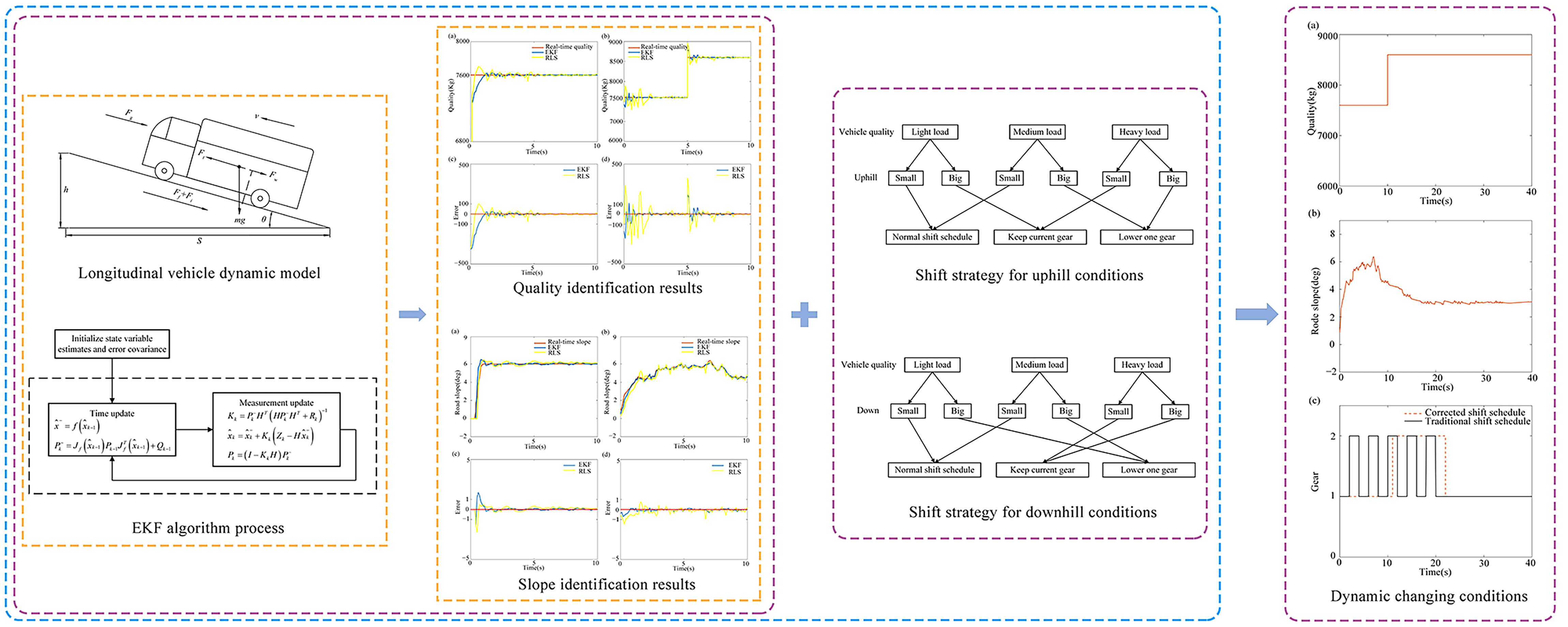
The extended Kalman filter (EKF) algorithm and acceleration sensor measurements were used to identify vehicle mass and road gradient in the work. Four different states of fixed mass, variable mass, fixed slope and variable slope were set to simulate real-time working conditions, respectively. A comprehensive electric commercial vehicle shifting strategy was formulated according to the identification results. The co-simulation results showed that, compared with the recursive least square (RLS) algorithm, the proposed algorithm could identify the real-time vehicle mass and road gradient quickly and accurately. The comprehensive shifting strategy formulated had the following advantages, e.g., avoiding frequent shifting of vehicles up the hill, making full use of motor braking down the hill, and improving the overall performance of vehicles.Graphic Abstract
Keywords
The large-scale popularization of pure electric vehicles has been recognized worldwide to improve the worsening environmental problems. The transmission system of pure electric vehicles tends to be two-shift gears or multiple gears for enhancing the power of electric vehicles [1]. Traditional two-parameter and three-parameter shifting laws do not consider the changes in vehicle quality and road gradient, especially for heavy-duty commercial vehicles. Meanwhile, the mass of electric commercial vehicles may vary by up to 400% depending on load conditions [2]. Shift control strategies for different load ranges are also different, which significantly affects the economic performance of vehicles. Adjusting the shift control strategy online according to vehicle mass can make the vehicle run more smoothly during automatic shifts, and get a more economical shift control strategy. Likewise, the road slope is also an important source of a longitudinally dynamic external load of heavy commercial vehicles. Hilly areas occupy 69% of the total land area, and mountain ramps are a common road condition for commercial vehicles in China [3]. The identification of road slopes can improve the overall performance of automatic transmission and prevent the failure of automatic transmission in the climbing condition. Therefore, heavy vehicle mass and road slopes are two important vehicle control inputs. It is of great significance to accurately identify the vehicle mass and road slopes to correct the shifting rule and improve the adaptability of vehicle shifting [4].
Mahyuddin et al. [5] proposed a novel observer-based parameter estimation scheme with a sliding mode to estimate the road gradient. The vehicle weight only uses the vehicle’s velocity and driving torque, the estimation is not accurate and the error is large. McIntyre et al. [6] proposed a two-stage estimation strategy for determining the mass of heavy vehicles and road grades. However, the estimation of time-varying road slopes by the method requires a separate estimator, which leads to complex algorithm and a large number of calculations. Holm [7] adopted the extended Kalman filter to estimate vehicle mass and road slopes, but this method requires a large number of calculations. Lei et al. [8] used the extended Kalman filter algorithm to estimate vehicle mass and road slopes. However, this algorithm has a large number of calculations, and the coupling problem between mass and road slopes is not effectively solved. Li et al. [9] proposed a two-layer based adaptive parameter estimator to estimate the vehicle mass and road slopes under longitudinal moving conditions. Additional sensors are not required, which saves the cost. However, the method still has a large number of calculations, and the joint quality and road slope models lead to the mutual input of the two estimation results, which affect each other, and the accuracy is poor. Wenbo et al. [10] presented a vehicle mass estimation method based on high-frequency information extraction to improve existing mass estimation methods that are susceptible to road slopes with poor real-time performance. But the result depends on the extraction of high frequency information. Kim et al. [11] proposed a recursive least square algorithm to estimate road grades and vehicle mass, but this algorithm only considers the sensors in the vehicle, which is limited and cannot be promoted on a large scale. Shen et al. [12] addressed parallel vehicle mass and road grade estimation problems with a Bayesian inversion-based approach, but the calculation is heavy and the algorithm is complicated. The above studies have the problems of a large number of calculations and coupling of the two identification parameters in the road slope identification.
There are also some studies on shift strategies combining vehicle mass and road slope recognition. Lu et al. [13] proposed a slope recognition method based on the vehicle’s acceleration and used genetic algorithm to modify the traditional shift schedule. But there is a time error in this method. Liu et al. [14] proposed an intelligent shift control method based on road roughness recognition according to vehicle dynamics, and modified the shift point by establishing a shift control model. However, the slope recognition accuracy is not high, which leads to the phenomenon of delay in gear shifting. Li et al. [15] obtained the comprehensive shift strategy under different vehicle masses and road gradients by solving the hierarchical gravity search algorithm. While the shift cycle can be eliminated, there are still issues with shift shock and torque ripple. The above research does not completely solve the problem of shift shock and frequency in modifying the shifting strategy.
The EKF algorithm was used to identify the vehicle mass, and then the acceleration sensor was combined to measure road slopes in the work. It cleverly avoids the coupling problem between the identified quality and slope calculations in the above study. Next, shifting rules of electric commercial vehicles were dynamically corrected according to the identification results of vehicle mass and road gradients, which effectively avoided the problem of frequent shifting of automatic transmissions due to dynamic changes in vehicle mass and road gradients. Besides, the recursive least squares (RLS) algorithm with a forgetting factor is introduced to compare the accuracy of the proposed algorithm.
2 Vehicle Mass and Road Slope Identification Based on EKF Algorithm
2.1 Longitudinal Vehicle Dynamics
The vehicle is regarded as a rigid body in the process of driving uphill, and Newton’s second law is used to analyze its force (see Fig. 1).
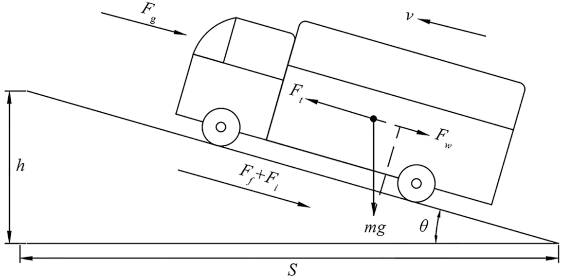
Figure 1: Longitudinal vehicle dynamic model
According to Newton’s second law, the longitudinal dynamics model of vehicles is as follows [16]:
where Ft, Ff, Ft, Fw and Fg are the driving force, rolling friction force, gradient resistance, aerodynamic resistance and uphill driving force, respectively. They are defined as
where Te is the actual input torque from the motor to the transmission, ig is the transmission ratio, i0 is the main reducer transmission ratio, ηT is the mechanical efficiency of the transmission, r is the rolling radius, m is the mass of the vehicle, f is the rolling resistance coefficient, θ is the angle of gradient, CD is the air density coefficient, A is the vehicle frontal area, ρ is the air density, ν is the longitudinal speed of the vehicle, δ is the automobile rotation mass conversion coefficient, dν/dt is the longitudinal acceleration of the vehicle.
The nonlinear equation of the vehicle’s longitudinal dynamics is expressed as
where
According to road design specifications [17], the maximum longitudinal slope of the expressway plain micro-hill area is 3%, the mountain hilly area is 5%, the maximum slope of the plain micro-hill area of the first-class vehicle-specific highway is 4%. The hilly area is 6%, the general four-level highway is 5% in the plain micro-hill area, and the mountain area is 9%. Therefore, the general road slope is small. So
2.2 Extended Kalman Filter Principle
Kalman filtering is an optimal estimation algorithm that removes noise from changing data and predicts the future output of the system. It has the advantages of easy programming and real-time update of field collected data. It is widely used in Communication, Navigation, Guidance and Control [18]. Kalman filtering is only applied to state estimations for linear systems, while the EKF algorithm is used for nonlinear systems. The EKF algorithm performs the Taylor expansion of the nonlinear function, then omits the higher-order term and retains the first-order term of the expansion term, which linearizes the nonlinear function. Finally, the state and variance estimations of the system are approximately calculated by the Kalman filter algorithm.
2.3 Vehicle Quality Status Observer
The vehicle mass state observer is designed based on the EKF algorithm. The selected system state variables are longitudinal speed ν, vehicle mass m. x(t) is the system state variable (i.e.,
Using the forward Euler method [20] to discretize Eq. (10) can obtain, the system discretization equation,
The system process noise and measurement noise are selected as Gaussian white noises with zero mean and independent of each other. Wk, Qk, Vk and Rk are the system process noise, the covariance, the measurement noise and the covariance, respectively.
Based on Eq. (11), the state equation of the system [21] can be obtained as
The system measurement equation is
The state space expression of the system [22] is
where H is the measurement matrix.
The EKF algorithm is divided into time and measurement updates [2]. The time update equation uses the previous state to predict the estimated value and estimated covariance matrix of the next state. The measurement update equation calculates the Kalman gain. By updating and iterating in this way, the best estimate can be calculated. Its algorithm flow see Fig. 2.
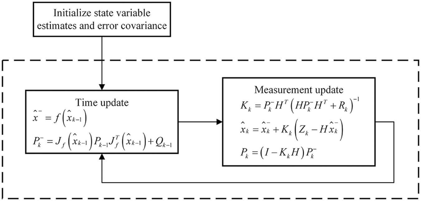
Figure 2: EKF algorithm process
The Jacobian matrix in the quality estimation algorithm [23] is expressed as
There are three methods for real-time estimation of road gradients, which are using CAN bus information and driving equations, using GPS elevation information and adding an acceleration sensor to estimate road gradient, respectively [24]. The kinematics method is used to estimate the road gradient in the work. The on-board acceleration sensor is installed on the electric commercial vehicle, and sensor measurement data are filtered and analyzed by the EKF algorithm to identify the real-time gradient.
According to the kinematic equation [11],
where ax and
According to the above analysis of vehicle longitudinal dynamics (i.e.,
State variables of the selected system include vehicle speed ν, acceleration sensor measurement signals axand sinθ, and state variable of the system
The system state is
The vehicle speed of the system can be output through the simulation after the Δt time, and the observation equation defined as
Same as the quality identification of vehicles, system process noises and measurement noises are selected as Gaussian white noises with zero and independent of each other.
Supposing
where A is the process matrix
Road gradients are obtained by calculating and identifying according to the EKF algorithm flow of Fig. 2.
3 Shifting Regularity of Electric Vehicle Based on Vehicle Mass and Road Gradient Recognition
3.1 Electric Vehicle Shift Schedule
According to the number of control parameters of the automatic transmission, shifting law can be divided into single-parameter, double-parameter and three-parameter shift law [26]. Among them, the shift law with speed and accelerator pedal opening as control parameters are the most mature and most widely used shift law at present [27]. According to the different control objectives, the shifting law can be divided into dynamic shifting law and economical shifting law [28].
The work selected a two-speed AMT electric commercial vehicle with vehicle speed and accelerator pedal opening as control parameters. Optimal dynamic shifting law and optimal economical shifting law for electric commercial vehicles were formulated, respectively. The shift pattern was corrected by recognizing vehicle mass and road gradients.
Dynamic shifting law can make full use of the output torque of the motor, so that the vehicle always has sufficient backup power and the optimal dynamic performance of the vehicle is ensured. Acceleration was used as the dynamic index, and dynamic shifting law was formulated by the analytical method in the work. The intersection of two adjacent accelerations is taken as the optimal dynamic shift point under the optimal dynamic performance of vehicle.
Assuming that the road gradient is 0, vehicle acceleration can be obtained from Eq. (8) as
where m is the vehicle mass, and
The corresponding relationship between the driving motor speed and the vehicle speed is
Then a definite functional relationship exists between the output torque of the drive motor and the pedal opening, defined as
Eqs. (22)–(24) are used to obtain
According to Eq. (25), the acceleration curves of the first gear and the second gear under different pedal opening degrees can be drawn, as shown in Fig. 3a. The intersection of the first and second gear acceleration curves is the optimal dynamic shift point. If there is no intersection, the vehicle speed corresponding to the maximum motor safe speed of the current gear is selected as the optimal dynamic shift point. The upshift curve is obtained by connecting the acceleration intersection points of two adjacent gears under different accelerator pedal opening degrees into a curve, The downshift curve is obtained by the equal delay method, see Fig. 3b.
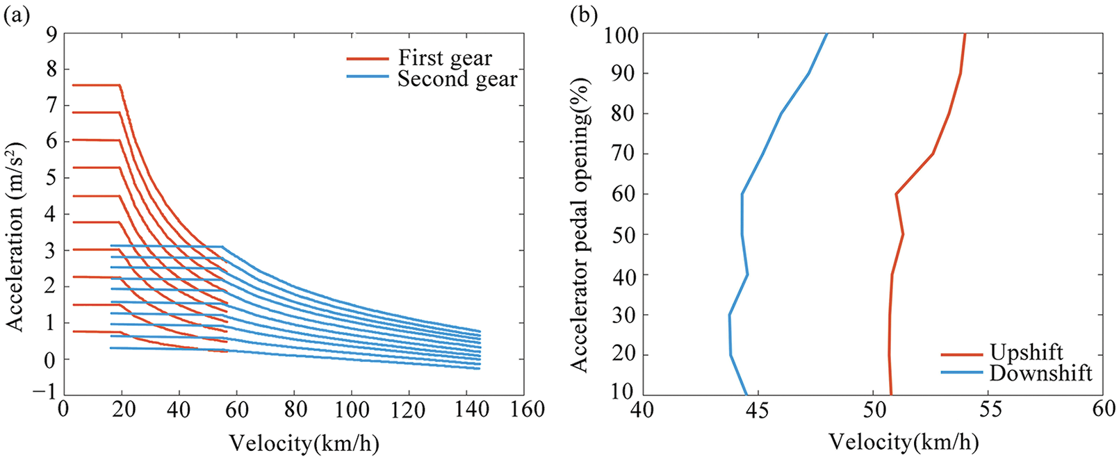
Figure 3: (a) The first and second gear acceleration curves of different pedal openings, and (b) Optimum dynamic shift curve
Economic shift law refers to the shifting law that can minimize energy loss and ensure the optimal economic performance of the vehicle on the premise of meeting power required by normal driving. The economical shifting law is obtained by the motor efficiency curve. The MAP of motor characteristics is an important basis for formulating the optimal economic shifting law. The MAP of the motor (see Fig. 4) can be expressed as
where
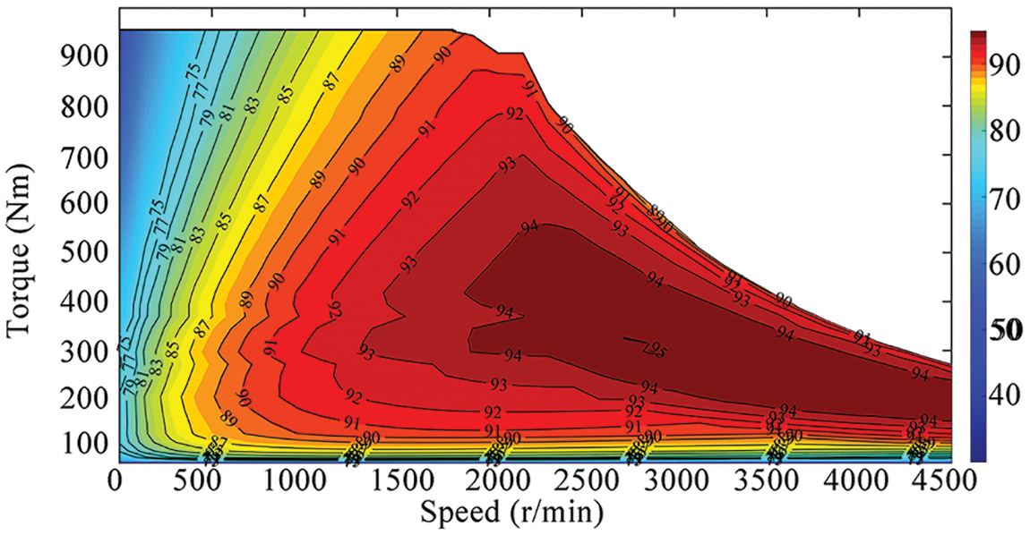
Figure 4: Motor efficiencies
The efficiency curves of the first gear and the second gear with different pedal openings need to be calculated according to the MAP and the transmission parameters in calculating the optimal economical shifting point. Fig. 5a shows the efficiency curves for the first and second gears at the 40% pedal opening and the shifting speed [29]. Similarly, the shifting speeds at other pedal openings can be obtained, and then we can fit the optimal economic upshift curve. The vehicle speed of downshifting refers to the downshifting method in the above optimal dynamic shifting law to avoid frequent shifting. Then the optimal economical shifting law is obtained (see Fig. 5b).
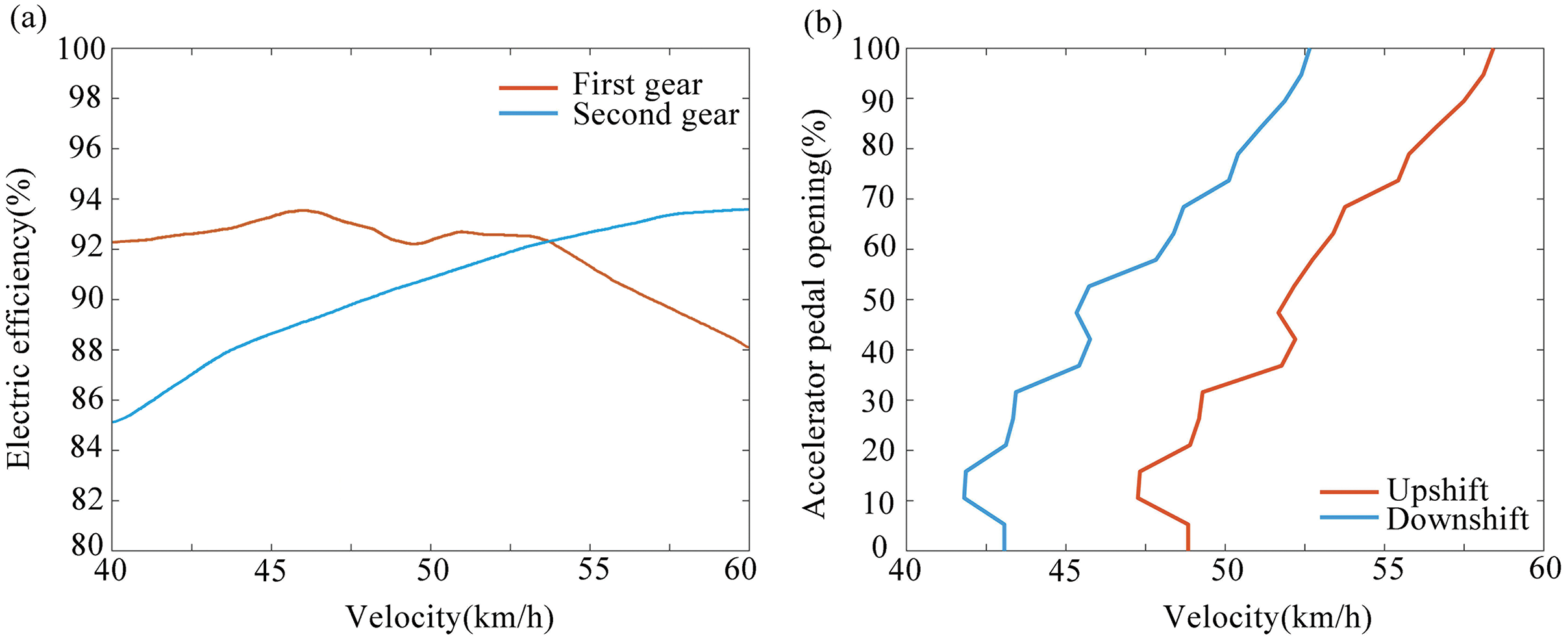
Figure 5: (a) Curve of the 40% accelerator pedal opening, and (b) Optimum economy shift curve
3.2 Comprehensive Shift Law Based on Mass and Gradient Recognition
Optimal dynamic shifting law and the optimal economical shifting law are formulated according to the operation condition of electric commercial vehicles on flat road. However, the number of electric commercial vehicles and the road gradients are in dynamic changes in the actual driving process. Failure to recognize in real-time will leads to frequent shifts of vehicles on ramps, excessive wear of shift components and other problems. Identified vehicle mass and road gradients should be used to correct the shifting pattern. According to the different qualities, and [30], this work creatively divided the vehicle quality into 3 grades. There are many ways to divide the range between no-load and full-load mass. we selected (
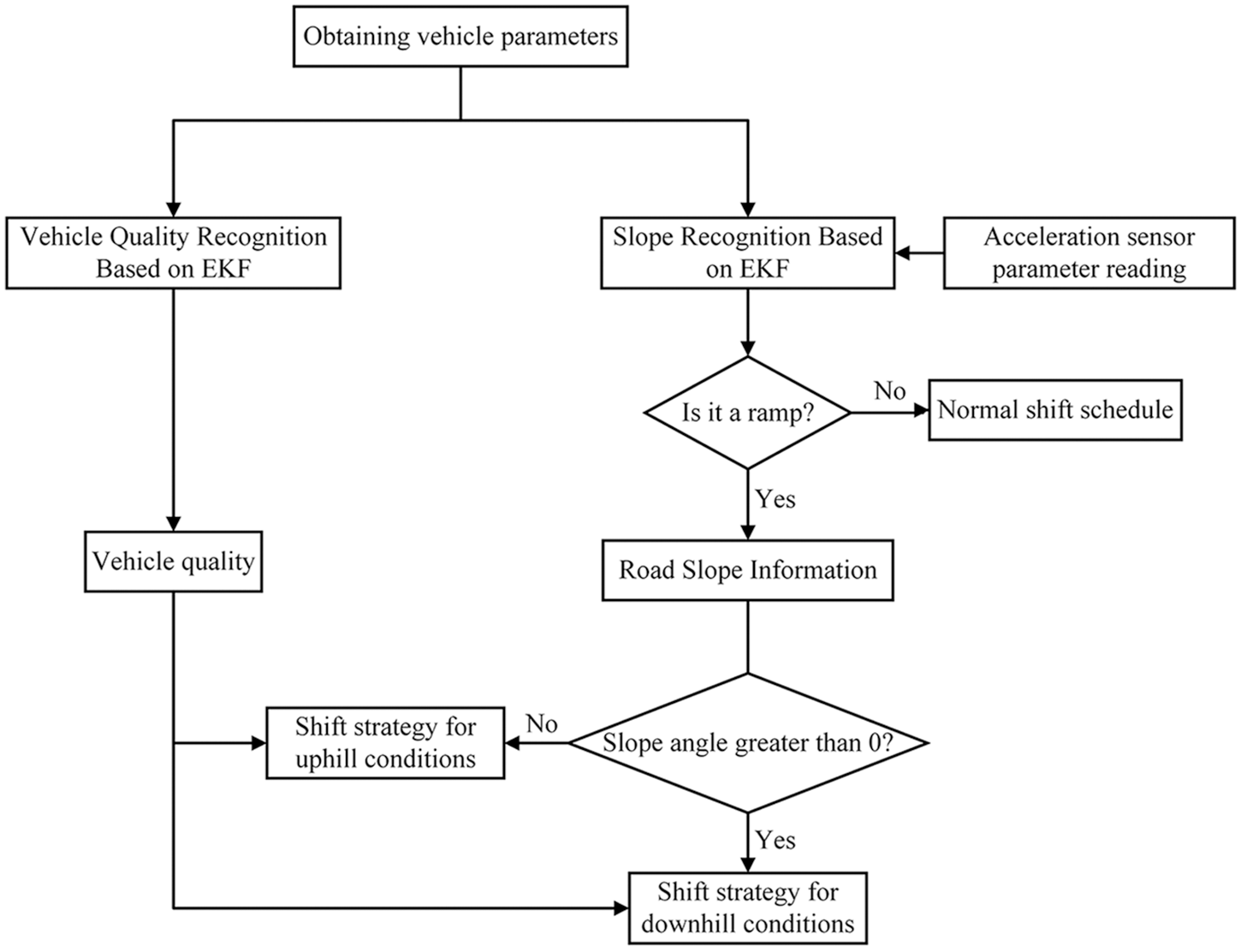
Figure 6: Shift strategy process by different ramp conditions
It is defined that when the vehicle driving gradient is greater than 0, it is an uphill condition (see Fig. 7) for the shifting strategy for uphill. When the vehicle is running on a small slope and the vehicle mass is light load or medium load, the shifting strategy is a normal regular shift. The vehicle mass is heavy load, the current gear is maintained. When recognizing that the car is driving on a large slope and the vehicle mass is medium or heavy, one should lower for climbing, the vehicle mass is light load, then the current gear is kept.
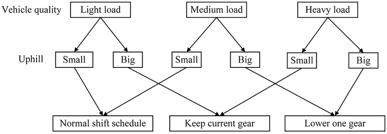
Figure 7: Shift strategy for uphill conditions
Similarly, when it is judged that the vehicle is in a downhill condition, the driving gradient is less than 0, a shifting strategy for downhill conditions is formulated (see Fig. 8). The downhill is also divided into a small gradient range (−9%, 0%) and large slope range (−17.6%, −9%). As the component force of the vehicle’s gravity is converted into the driving force when going downhill, the driver usually adopts braking to maintain the normal running of the vehicle. But this operation will lead to a high disc-brake friction temperature. The braking efficiency will decrease, and traffic accidents are prone to occur in serious cases [32]. Therefore, the drive motor should be used for auxiliary braking when going downhill. When it is identified that the vehicle is driving on a small slope and the vehicle mass is light load or medium load, the normal shift rule can be adopted. The current gear should be maintained when the vehicle mass is heavy load. The vehicle is driving on a large slope and the vehicle mass is light load or medium load, one gear is dropped. When the vehicle mass is heavy load, the current gear should run to prevent the absence of auxiliary braking during shifting, which improves the stability of the vehicle running downhill.
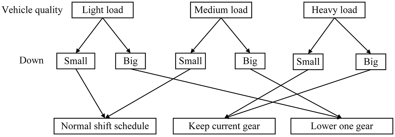
Figure 8: Shift strategy for downhill conditions
4.1 Simulation Platform Establishment
A complete vehicle model of an electric commercial vehicle on the AVL_CRUISE simulation platform is established to complete the vehicle simulation. Cruise simulation output data replaces actual output data, for example, speeds and motor torque are transmitted to Simulink through the interface. The EKF model is built in Simulink to simulate input data for co-simulation. Meanwhile, the actual situation of CAN bus data acquisition is considered to reflect the authenticity of collected data. Gaussian white noise was added to the vehicle speed and motor torque data in the Matlab environment. The added white Gaussian noise [33] is that the instantaneous value obeys the Gaussian distribution, and the power spectral density is uniformly distributed noise. Fig. 9 shows the co-simulation process. The RLS algorithm was also used for comparative analysis in the work, Forgetting factor λ assigns weights for old and new data and usually takes a constant value between 0.95 and 1 [31]. λ is the value of the forgetting factor fixed at 0.98 to give a better balance between accuracy and speeds [34]. The value of forgetting factor λ is set to 0.98.
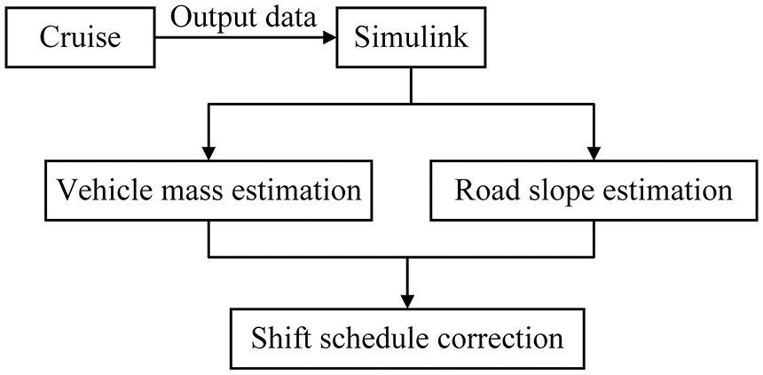
Figure 9: Co-simulation process
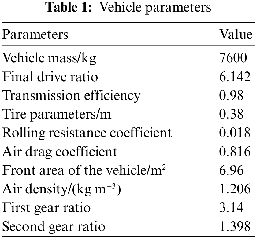
A company’s heavy-duty electric commercial vehicle is taken as an example for research. Its specifications are 5998 mm * 2200 mm * 3350 mm, the wheelbase is 3360 mm. An electric commercial vehicle model is built on the Cruise platform, (see Table 1 for vehicle parameters).
The power transmission system of the electric commercial vehicle in the work is composed of a power transmission integrated controller, a power battery, a permanent magnet synchronous motor, a two-speed AMT and a differential. Fig. 10 shows the power transmission system. The transmission used is two Gear AMT power transmission, due to the fast response of the drive motor, and the two-gear AMT adopts a no-clutch structure (see Fig. 11 for the specific structure). The adopted two-gear AMT consists of two sets of meshing gears, a synchronizer, a shift motor and a differential for two gears. One of the gears is combined at a time for shifting.
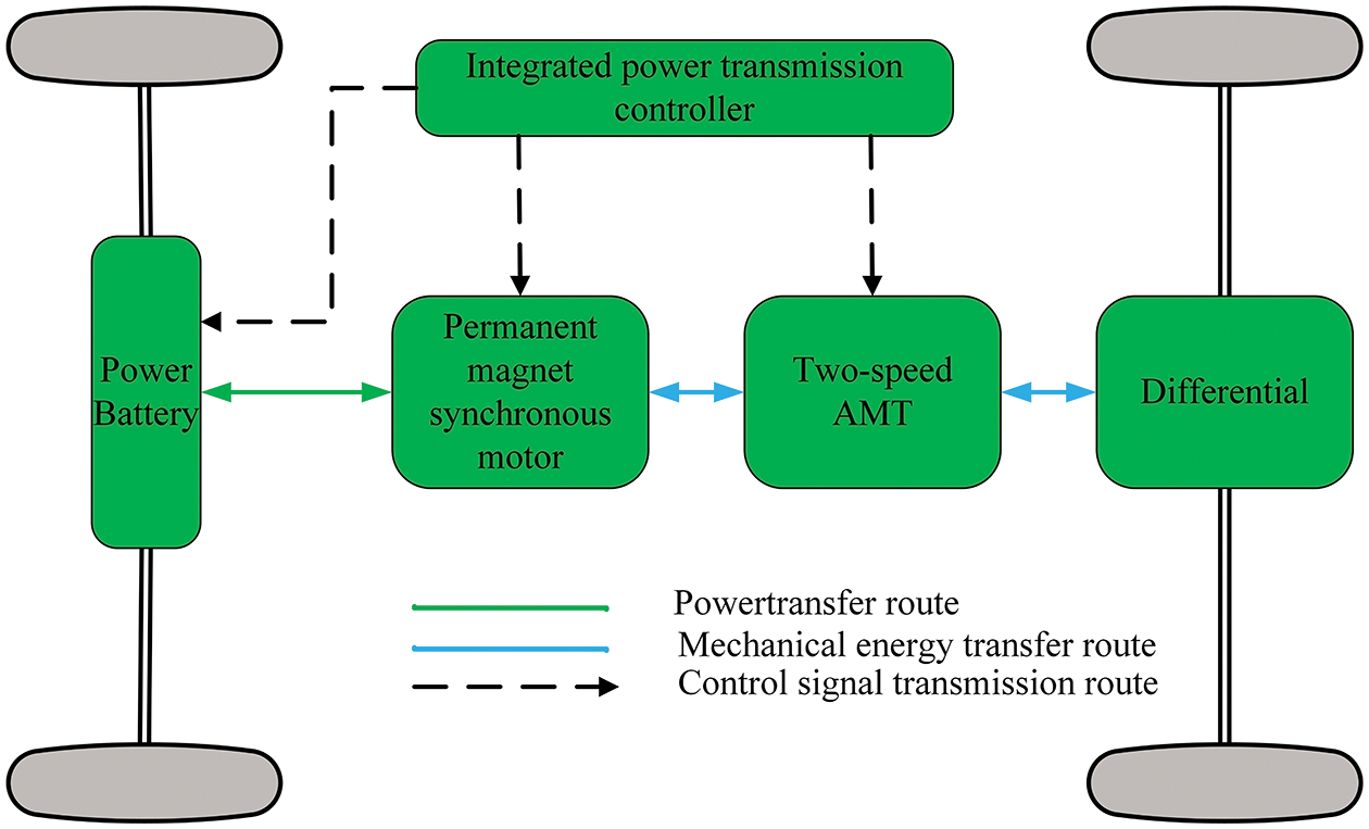
Figure 10: Power transmission system
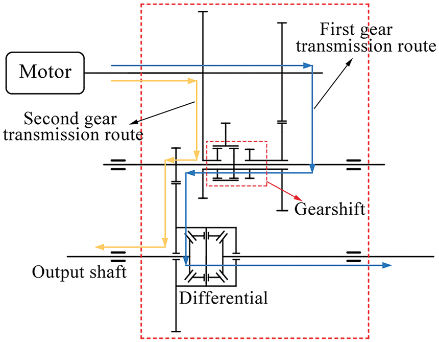
Figure 11: Two-gear AMT structure
4.2 Simulation Analysis of Vehicle Quality Recognition
The vehicle quality is divided into the fixed quality stage and variable quality stage to verify the accuracy of the proposed quality identification algorithm. In the fixed mass stage, the curb weight of electric commercial vehicles is set to 7600 kg. As the cargo quality of electric commercial vehicles does only changes during loading cargo. The electric vehicle is loaded with 1000 kg cargos with variable mass stage at 5 s, Figs. 12a and 12b show the EKF and RLS simulation results.
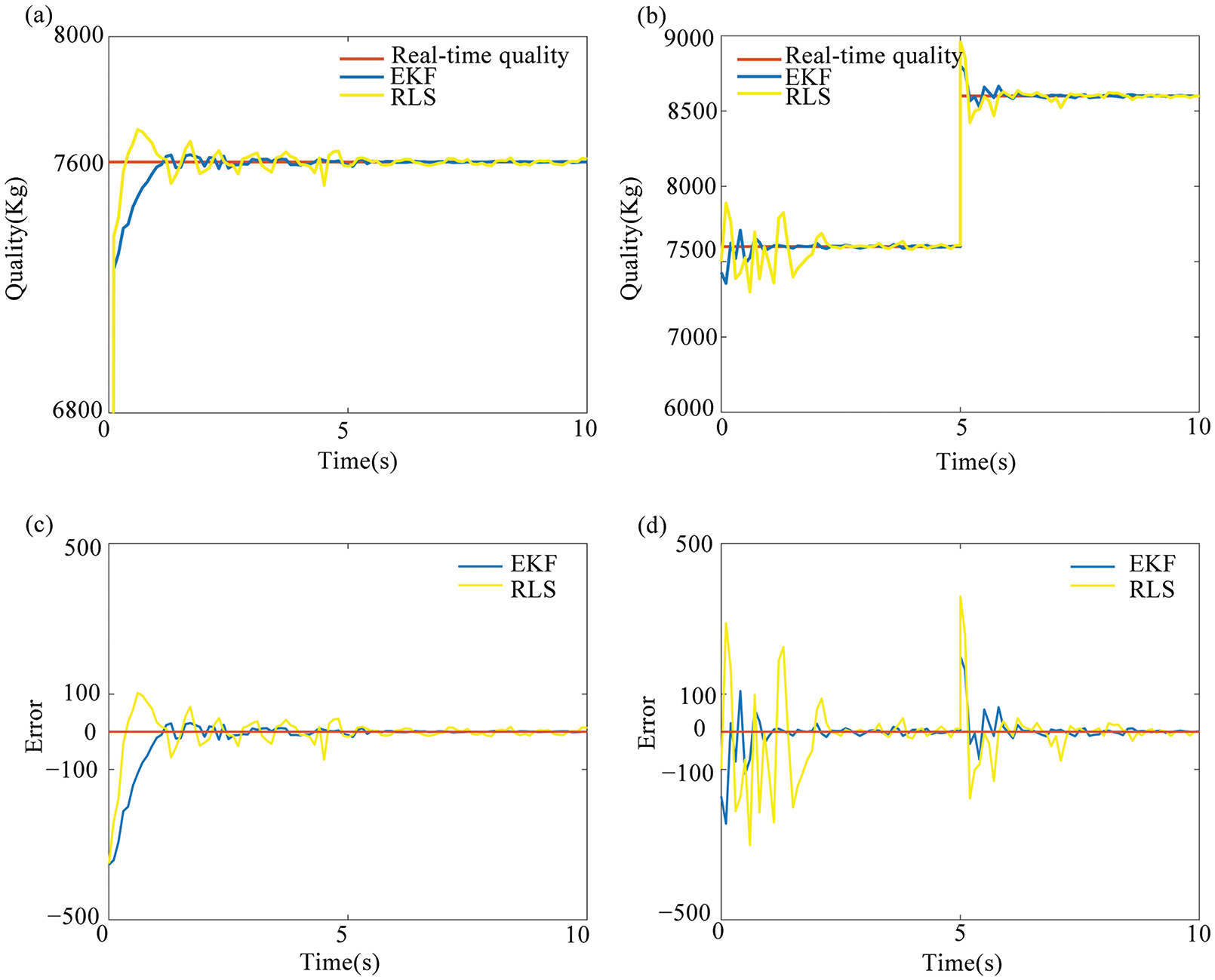
Figure 12: Quality identification results: (a) Fixed quality stage, (b) Variable quality stage, (c) Error of the fixed quality stage, and (d) Error of the variable quality stage
Both the EKF algorithm and the RLS algorithm fluctuate at an earlier time with the fixed quality (see Fig. 12c). However, the stabilization time of the EKF algorithm is shorter than that of the RLS algorithm, with a small identification error. Similarly, the EKF algorithm can still effectively identify the vehicle mass in a short time with variable qualities (see Fig. 13d), with small volatility. Compared with the RLS algorithm, the EKF algorithm can quickly identify the changing quality in a short time, it is recognized and stabilized for a short time when there is a quality step. In general, the EKF algorithm is more suitable for identifying the changing quality in real time.
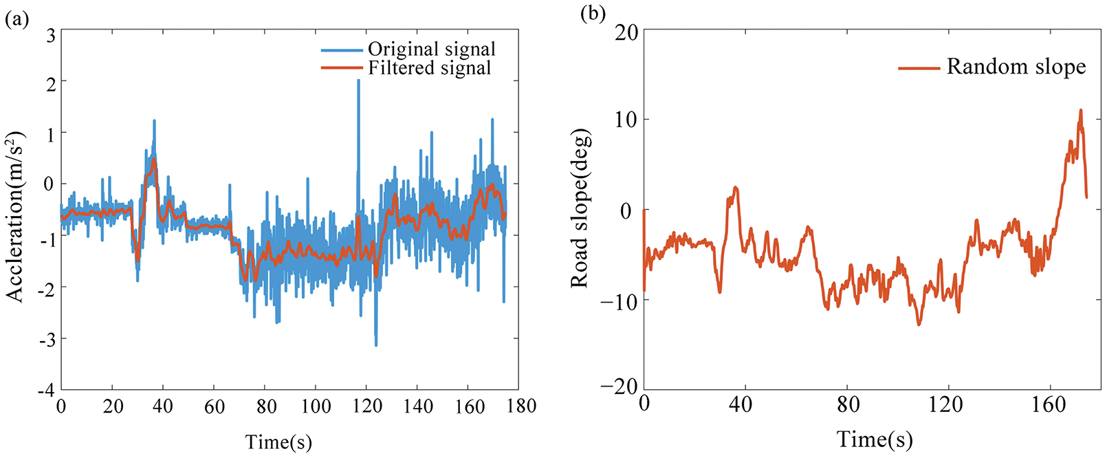
Figure 13: (a) Acceleration signal filtering results, and (b) Random slope case
4.3 Road Slope Recognition Simulation Analysis
The EKF algorithm is used to filter the measurement signal of the acceleration sensor to remove noises due to the error in the sensor measurement. Fig. 13a shows the filtering effect. The blue line in the figure represents the measurement signal obtained from the acceleration sensor, and the red line represents the filtered signal. The measurement signal is well filtered by the EKF. According to filtered acceleration data, a road slope observer is designed to realize the dynamic recognition of the slope.
The fixed-slope road and variable-slope road conditions are constructed in the Cruise simulation environment, respectively to verify the estimation accuracy of the algorithm under different road conditions. Among them, the fixed-slope condition refers to the driving condition with better road surface conditions, where the road surface gradient changes smoothly with a stable change rate. The variable-slope road condition refers to the road section where the slope angle changes irregularly from 0. On account of simulate normal operating conditions, the fixed-slope condition is set as a section of uphill road with a fixed gradient (set to 6 deg) in the work. Fig. 13b shows the variation curve of the gradient angle of the variable-slope with time. The slope value greater than 0 is in the uphill section, while the slope value less than 0 is in the downhill section. The work takes 10 s as the simulation time for subsequent analysis.
Fig. 14 shows the recognition effect and error fluctuation of the EKF algorithm and the RLS algorithm on the fixed slope road and variable slope road sections, respectively. First, the EKF fluctuation frequency is smaller than that of RLS to the overall smoothness of the curve in the fixed slope road section. When the slope error range is stable within 0.2 deg, the stable condition is considered [4]. The EKF first reaches the stable condition, and the error fluctuation range is smaller than that of the RLS algorithm (see Fig. 14c). Secondly, the road gradient algorithm proposed in the work has stronger recognition and tracking capabilities for the variable slope road (see Fig. 14d). The EKF algorithm is smaller than the fluctuation range of the error curve, and the recognition effect is consistent with real-time changes. The slope curves are in good agreement and have high robustness.
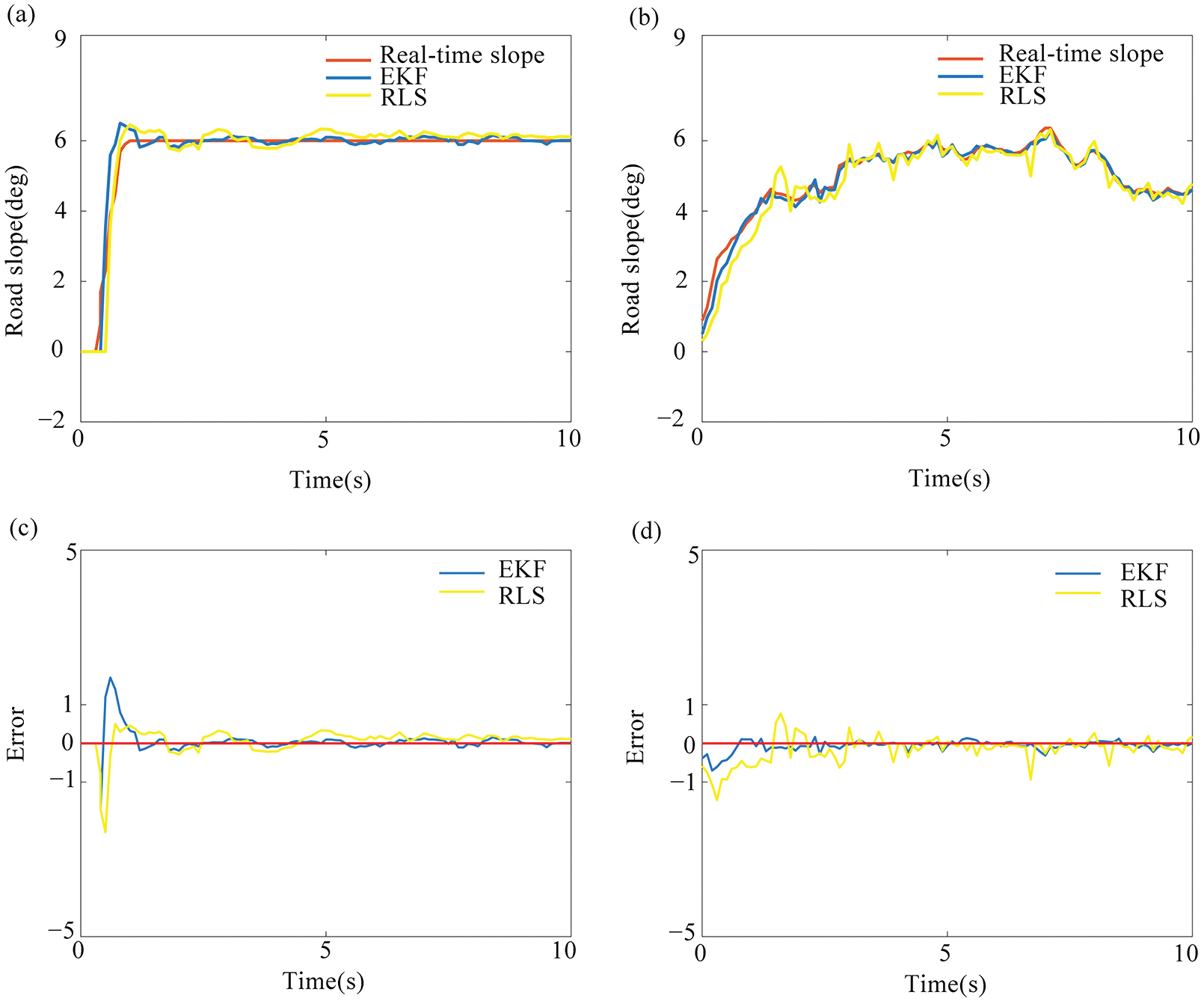
Figure 14: Slope identification results: (a) Fixed slope road, (b) Variable slope road, (c) Error of the fixed slope road, and (d) Error of the variable slope road
Based on the above analysis of the quality and slope identification results, identification effect data are processed in the form of the mean absolute error (MAE) and root mean square error (RMSE) (see Table 2). The results of vehicle mass and road slopes based on the hybrid algorithm of RLS and EKF to estimate are similar to the results of [35] in the quality identification, but the calculation amount is greatly reduced. Slope estimation accuracy is improved by about 12% in terms of RMSE in the variable slope identification results.
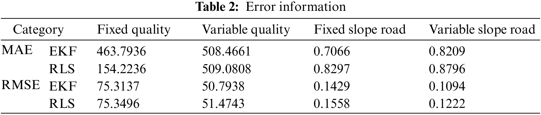
In summary, the EKF algorithm in the work to identify vehicle mass and the EKF algorithm combined with acceleration sensor measurement to identify road slope have fast convergence and accurate identification. The accurate identification of vehicle mass and road gradient for electric commercial vehicles, can be used to modify shifting strategies.
4.4 Simulation Analysis of the Revised Shifting Strategy
The accuracy of the revised shifting strategy is verified under fixed conditions. The speed of the car is set to 40 km/h, with the 2nd gear, a curb weight is 7600 kg, and the slope is 6 deg, respectively. The simulation is carried out under the above specific working conditions, and Fig. 15 shows the changing curve of the gear.
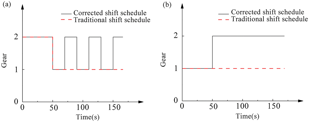
Figure 15: Shifting laws for road ramps: (a) Simulation results of uphill shift law, and (b) Simulation results of downhill shift law
Fig. 15a shows the shifting curve of the uphill condition. When the car is climbing in the 2nd gear, the component of the vehicle’s gravity turns into driving resistance under the traditional shifting law, which makes the car decelerate. To keeping the car driving at a constant speed, the acceleration pedal opening must be increased. If the downshift state of the 1st gear is reached, it will be downshifted to the 1st gear, and the vehicle speed will increase. After the vehicle speed increases, the vehicle will reduce the accelerator pedal opening in order to maintain a constant speed. At this time, if the upshift condition of the 2nd gear is reached, and it will be upshifted to the 2nd gear. However, when the accelerator pedal opening is increased and the speed decreases, the gear will be downshifted. Frequent upshifts and downshift are until the end of the uphill condition. It aggravates the friction of the shifting elements, reduces the service life of the transmission system, and worsens driving. Therefore, the car can identify the quality and slope of the vehicle using the revised shift rule on the slope during the climbing process, and comprehensively judge that it is down to 1st gear and limit the upshift. It can eliminate the phenomenon of frequent shifting and improves the ride comfort of the vehicle.
Fig. 15b shows the shifting curve under downhill conditions. The vehicle adopts the traditional shifting strategy. The vehicle maintains the 1st gear when driving on a long slope of 6 (deg), and the accelerator pedal opening is 0, the vehicle gravity component is converted into driving force and the vehicle speed increase. If the vehicle reaches the 2nd gear upshift condition, and the vehicle will up to the 2nd gear. The driver reduces the speed through the brake, and long-term use of deceleration brake will aggravate their wear. Therefore, the vehicle can identify the vehicle’s mass and slopes with the modified ramp strategy during the downhill process. It will comprehensively judge whether maintain the current gear, and make full use of auxiliary braking force provided by the drive motor for braking, and improve the safety of vehicles driving on ramps.
Next, we establish a random operating condition (see Figs. 16a and 16b), to verify the effectiveness of the shifting strategy under random operating conditions. Vehicle mass is set to be 7600 kg in an unloaded state at the beginning, and a load of 2000 kg is added at 10 s to realize the dynamic change of the vehicle mass. The road gradient is set to dynamically change from the initial uphill to the downhill section in about 8 s, and stabilizes at a gradient of 3 deg about 20 s. The simulation verification is carried out (see Fig. 16c). When the vehicle accelerates from a standstill and a no-load state, when entering a ramp, the transmission gears of the vehicle are all in the 1st gear under the control of the revised shifting strategy during the climbing process. While the traditional shifting law cannot adapt to the dynamically changing road grades, which causes the transmission to frequently switch between first and second gears. The vehicle starts to enter the downhill section at 8 s, and the road gradient gradually decreases to 3 deg. The vehicle load increases by 2000 kg at 10 s. According to the shifting rule after the real-time results of the identification of the vehicle load and road gradient, when the transmission is upgraded to the 2nd gear, there is a certain delay compared with the traditional shifting pattern. Similarly, the road gradient is stable at 3 deg and about 20 s, and the transmission is lowered to the 1st gear.
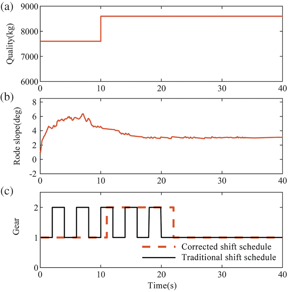
Figure 16: Dynamic changing conditions: (a) Variable quality stage, (b) Variable slope road, and (c) Simulation results of shift schedule
Shift points mentioned in the work are delayed compared with the traditional shift schedule, because the shift points are dynamically corrected according to the vehicle dynamic load and dynamic road gradient changes, thereby improving the vehicle’s adaptability to actual load changes and road gradient changes. The revised shifting strategy proposed in the work can select the optimal gear according to the actual vehicle load or road gradient. The algorithm is simple, and the amount of calculation is small. It can effectively avoid the accidental shifting of the vehicle due to changes in the load or road gradient, and improve the adaptability of the vehicle to the driving environment.
The work aimed at the problem that it was difficult to identify the real-time changes in vehicle mass and road slope in the shift control system of electric commercial vehicles. The real-time identification of the fixed quality, variable quality, fixed slope and variable slope are studied. The EKF algorithm, combined with the acceleration sensor measurement, was used to identify the vehicle mass and road gradient. According to the real-time identification results, the shifting law of electric vehicles was dynamically corrected. The co-simulation analysis was carried out, and the conclusions are as follows:
1) Compared with the RLS algorithm, the EKF algorithm had a faster identification speed and higher accuracy with fixed mass. The EKF algorithm could identify faster, and the volatility was small with variable mass.
2) The recognition accuracy of the EKF algorithm and RLS algorithm was comparable for fixed-slope road conditions. Compared with the RLS algorithm, the proposed algorithm had stronger identification and tracking performance, a smaller fluctuation range and better robustness for variable-slope road conditions.
3) The modified gear shift strategy selected the appropriate gear according to the identified vehicle mass and road slopes. When the vehicle is going uphill, it can effectively avoid shifting cycles, reduce the number of shifting, and reduce brake wear when the vehicle is going downhill. The smoothness of the gear shift of the vehicle was improved.
The modified gear shift strategy proposed in this paper is suitable for working conditions with slow gradient change. For unusually complex working conditions, shifting strategy is still a problem to be solved. This is also one of the main works of future study.
Funding Statement: This research was funded by the Innovation-Driven Development Special Fund Project of Guangxi, Grant No. Guike AA22068060, the Science and Technology Planning Project of Liuzhou, Grant No. 2021AAA0112 and the Liudong Science and Technology Project, Grant No. 20210117.
Conflicts of Interest: The authors declare that they have no conflicts of interest to report regarding the present study.
References
1. Ruan, J., Walker, P., Zhang, N. (2016). A comparative study energy consumption and costs of battery electric vehicle transmissions. Applied Energy, 165, 119–134. https://doi.org/10.1016/j.apenergy.2015.12.081 [Google Scholar] [CrossRef]
2. Kidambi, N., Harne, R., Fujii, Y., Pietron, G. M., Wang, K. (2014). Methods in vehicle mass and road grade estimation. SAE International Journal of Passenger Cars-Mechanical Systems, 7(3), 981–991. https://doi.org/10.4271/2014-01-0111 [Google Scholar] [CrossRef]
3. Meng, F., Jin, H. (2018). Slope shift strategy for automatic transmission vehicles based on the road gradient. International Journal of Automotive Technology, 19(3), 509–521. https://doi.org/10.1007/s12239-018-0049-5 [Google Scholar] [CrossRef]
4. Vahidi, A., Stefanopoulou, A., Peng, H. (2005). Recursive least squares with forgetting for online estimation of vehicle mass and road grade: Theory and experiments. Vehicle System Dynamics, 43(1), 31–55. https://doi.org/10.1080/00423110412331290446 [Google Scholar] [CrossRef]
5. Mahyuddin, M. N., Na, J., Herrmann, G., Ren, X., Barber, P. (2013). Adaptive observer-based parameter estimation with application to road gradient and vehicle mass estimation. IEEE Transactions on Industrial Electronics, 61(6), 2851–2863. https://doi.org/10.1109/TIE.2013.2276020 [Google Scholar] [CrossRef]
6. McIntyre, M. L., Ghotikar, T. J., Vahidi, A., Song, X., Dawson, D. M. (2009). A two-stage lyapunov-based estimator for estimation of vehicle mass and road grade. IEEE Transactions on Vehicular Technology, 58(7), 3177–3185. https://doi.org/10.1109/TVT.2009.2014385 [Google Scholar] [CrossRef]
7. Holm, E. J. (2011). Vehicle mass and road grade estimation using kalman filter. Institutionen for Systemteknik, Department of Electrical Engineering. [Google Scholar]
8. Lei, Y., Fu, Y., Liu, K., Zeng, H., Zhang, Y. (2014). Vehicle mass and road grade estimation based on extended kalman filter. Trans. Journal of the Chinese Society of Mechanical Engineers, 45, 9–13. [Google Scholar]
9. Li, B., Zhang, J., Du, H., Li, W. (2017). Two-layer structure based adaptive estimation for vehicle mass and road slope under longitudinal motion. Measurement, 95, 439–455. https://doi.org/10.1016/j.measurement.2016.10.045 [Google Scholar] [CrossRef]
10. Chu, W. B., Luo, Y. G., Luo, J., Li, K. Q. (2015). Vehicle mass and road slope estimates for electric vehicles. Journal of Tsinghua University (Science and Technology), 54(6), 724–728. [Google Scholar]
11. Kim, S., Shin, K., Yoo, C., Huh, K. (2017). Development of algorithms for commercial vehicle mass and road grade estimation. International Journal of Automotive Technology, 18(6), 1077–1083. https://doi.org/10.1007/s12239-017-0105-6 [Google Scholar] [CrossRef]
12. Shen, X., Zhang, Y. (2021). Estimating vehicle mass and road grade through Bayesian inversion. IFAC-PapersOnLine, 54(10), 235–240. https://doi.org/10.1016/j.ifacol.2021.10.169 [Google Scholar] [CrossRef]
13. Lu, H., Yin, X., Wu, X. (2015). Shift schedule modification for automated manual transmission based on road slope identification. 2015 International Conference on Electrical, Automation and Mechanical Engineering, pp. 124–127. Phuket, Thailand. [Google Scholar]
14. Liu, P., Liu, B., Dong, T., Zhang, C. (2017). Road roughness identification and shift control study for a heavy-duty powertrain. Energy Procedia, 105, 2885–2890. https://doi.org/10.1016/j.egypro.2017.03.645 [Google Scholar] [CrossRef]
15. Li, C., Zhang, C., Qu, S., Hu, Z. (2021). Comprehensive gear shift schedule of PELV considering road gradients and vehicle loads. China Mechanical Engineering, 32(3), 275. [Google Scholar]
16. Rhode, S., Gauterin, F. (2012). Vehicle mass estimation using a total least-squares approach. International IEEE Conference on Intelligent, pp. 1584–1589. Anchorage, AK, USA. [Google Scholar]
17. Cheng, A., Xiong, Q., Wang, L., Zhang, Y. (2019). Design of drive control strategy for mini pure electric vehicles on the condition of slope climbing. 2019 Chinese Control and Decision Conference (CCDC), pp. 4828–4832. Nanchang, China. [Google Scholar]
18. Li, Q., Li, R., Ji, K., Dai, W. (2015). Kalman filter and its application. Proceedings of the 2015 8th International Conference on Intelligent Networks and Intelligent Systems (ICINIS), pp. 74–77. Tianjin, China. [Google Scholar]
19. Wragge-Morley, R., Herrmann, G., Barber, P., Burgess, S. (2015). Gradient and mass estimation from CAN based data for a light passenger car. SAE International Journal of Passenger Cars-Electronic and Electrical Systems, 8(1), 137–145. https://doi.org/10.4271/2015-01-0201 [Google Scholar] [CrossRef]
20. Simon, D. (2006). Optimal state estimation: Kalman, H infinity, and nonlinear approaches. Hoboken: John Wiley & Sons. [Google Scholar]
21. Bishop, G., Welch, G. (2001). An introduction to the kalman filter. Proceeding of SIGGRAPH, Course, 8(27599–23175), 41. [Google Scholar]
22. Liao, X., Huang, Q., Sun, D., Liu, W., Han, W. (2017). Real-time road slope estimation based on adaptive extended kalman filter algorithm with in-vehicle data. Proceedings of the 2017 29th Chinese Control and Decision Conference (CCDC), pp. 6889–6894. Chongqing, China. [Google Scholar]
23. Wenzel, T. A., Burnham, K., Blundell, M., Williams, R. (2006). Dual extended kalman filter for vehicle state and parameter estimation. Vehicle System Dynamics, 44(2), 153–171. https://doi.org/10.1080/00423110500385949 [Google Scholar] [CrossRef]
24. Fathy, H. K., Kang, D., Stein, J. L. (2008). Online vehicle mass estimation using recursive least squares and supervisory data extraction. 2008 American Control Conference, pp. 1842–1848. Seattle, WA. [Google Scholar]
25. Lingman, P., Schmidtbauer, B. (2002). Road slope and vehicle mass estimation using kalman filtering. Vehicle System Dynamics, 37, 12–23. https://doi.org/10.1080/00423114.2002.11666217 [Google Scholar] [CrossRef]
26. Shen, P., Zhao, Z., Li, J., Guo, Q. (2020). Development of adaptive gear shifting strategies of automatic transmission for plug-in hybrid electric commuting vehicle based on optimal energy economy. Proceedings of the Institution of Mechanical Engineers, Part D: Journal of Automobile Engineering, 234(4), 1098–1112. https://doi.org/10.1177/0954407019864209 [Google Scholar] [CrossRef]
27. Tian, Y., Ruan, J., Zhang, N., Wu, J., Walker, P. (2018). Modelling and control of a novel two-speed transmission for electric vehicles. Mechanism and Machine Theory, 127, 13–32. https://doi.org/10.1016/j.mechmachtheory.2018.04.023 [Google Scholar] [CrossRef]
28. Jeoung, D., Min, K., Sunwoo, M. (2020). Automatic transmission shift strategy based on greedy algorithm using predicted velocity. International Journal of Automotive Technology, 21(1), 159–168. https://doi.org/10.1007/s12239-020-0016-9 [Google Scholar] [CrossRef]
29. Kawaguchi, S., Fukuyama, Y. (2016). Reactive tabu search for Job-shop scheduling problems considering peak shift of electric power energy consumption. Proceedings of the IEEE Region 10 International Conference (TENCON), pp. 3406–3409. Singapore. [Google Scholar]
30. Qu, J., Liu, D. (2009). An optimal method for dynamic three-parameter fuel economy shift schedule of AMT. 2009 International Conference on Information Engineering and Computer Science, pp. 1–4. Wuhan, China. [Google Scholar]
31. Xu, W., Xu, J., Yan, X. (2020). Lithium-ion battery state of charge and parameters joint estimation using cubature kalman filter and particle filter. Journal of Power Electronics, 20(1), 292–307. https://doi.org/10.1007/s43236-019-00023-4 [Google Scholar] [CrossRef]
32. Guo, Y., Fu, R., Yang, P., Yuan, W. (2006). Numerical simulation and calculation for transient thermal field of drum brake. Journal of Chang’an University (Natural Science Edition), 26, 87–90. [Google Scholar]
33. DjuriC, P. M. (1996). A model selection rule for sinusoids in white Gaussian noise. IEEE Transactions on Signal Processing, 44(7), 1744–1751. https://doi.org/10.1109/78.510621 [Google Scholar] [CrossRef]
34. Elmarghichi, M., Bouzi, M., Ettalabi, N. (2020). Robust parameter estimation of an electric vehicle lithium-ion battery using adaptive forgetting factor recursive least squares. International Journal of Intelligent Engineering and Systems, 13(5). https://doi.org/10.22266/ijies2020.1031.08 [Google Scholar] [CrossRef]
35. Sun, Y., Li, L., Yan, B., Yang, C., Tang, G. (2016). A hybrid algorithm combining EKF and RLS in synchronous estimation of road grade and vehicle’ mass for a hybrid electric bus. Mechanical Systems and Signal Processing, 68, 416–430. [Google Scholar]
Cite This Article
 Copyright © 2023 The Author(s). Published by Tech Science Press.
This work is licensed under a Creative Commons Attribution 4.0 International License , which permits unrestricted use, distribution, and reproduction in any medium, provided the original work is properly cited.
 Downloads
 Citation Tools