Numerical Stability and Accuracy of Contact Angle Schemes in Pseudopotential Lattice Boltzmann Model for Simulating Static Wetting and Dynamic Wetting

1  Introduction

The wetting phenomenon is not only widespread in nature but also plays an important role in the industry [1–3]. Solid wall wettability is characterized by the contact angle, which can loosely be defined as the affinity of the solid wall for the aqueous phase or non-aqueous phase. In oil recovery, a stable water film separating the oil and rock surface is desired for enhancing oil recoveries, so the wettability of the porous rock surface plays a profound role in the efficiency of oil recovery by waterflooding [4]. Fluid transport in porous media is a common problem in petroleum and hydraulic engineering, which is closely associated with dynamic wetting of the solid wall and the capillary-driven flow [5]. In the inkjet printing process, wettability patterns on a substrate can manipulate colloidal droplet motion, colloidal droplet coalescence as well as colloidal particles deposition mode, thus many different customized micro-structures or micro-patterns can be manufactured by the design of substrate wettability [6–8]. In the multiphase flow and heat transfer process, solid wall wettability not only plays a vital role in fluid transport efficiency [9] but also has significant impacts on nucleation energy barriers of phase-change heat transfer [10]. There are many other applications of the wettability phenomenon to name but a few [11,12], e.g., self-cleaning, water harvesting, geologic CO2 storage and etc.

Lattice Boltzmann method (LBM) is a mesoscopic numerical method based on kinetic theory, which preserves microscopic kinetic principles to recover macroscopic hydrodynamics. Fluid dynamics are described by microfluid particle movement governed by the LB equation, which two processes can solve: collision and streaming process [13]. The LBM has many superiorities in simulating multiphase flow problems [14–18], e.g., no need for tracking multiphase interface, easy handling of complex geometry and wall wettability. The pseudopotential LB model is the most widely used LB model, which was originally proposed by Shan et al. [19] by introducing a “effective mass” (or “pseudopotential”) at every fluid node to simulate fluid-fluid interaction force among fluid particles. By adding a fluid-solid interaction force near the wall in the pseudopotential LB model, multiphase flow problems involving solid wall wettability (e.g., multiphase flow in porous media, boiling and evaporation [20]) can be simulated. The numerical implementation in simulating solid wall wettability is named as “contact angle scheme”.

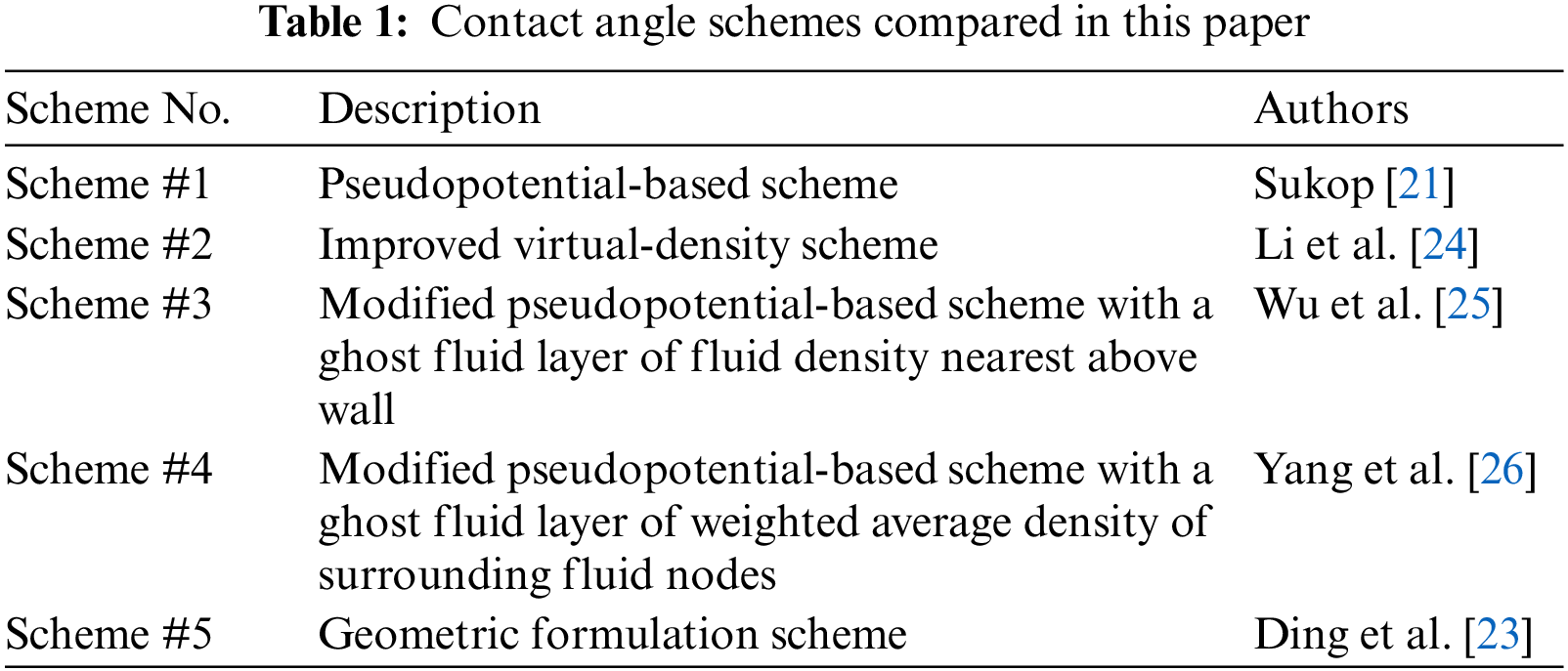
There are mainly five kinds of widely used contact angle schemes in the pseudopotential LB model. Sukop et al. [21] indicated that the fluid-solid interaction force can be calculated similarly to the fluid-fluid interaction force, and they proposed a contact angle scheme based on pseudopotential of fluid particles. This contact angle scheme was called “pseudopotential-based contact angle scheme” (PB scheme) by Li et al. [22]. Subsequently, Li et al. [22] modified the “pseudopotential-based contact angle scheme” to be of better performance for simulating large contact angles θ>90∘. The implementation of “pseudopotential-based contact angle scheme” or its modified scheme is inconvenient because several numerical tests are required to simulate a prescribed contact angle. Ding et al. [23] proposed a more straightforward contact angle scheme, which is based on the geometric formulation. The geometric formulation contact angle scheme (GF scheme) can simulate the contact angle with the prescribed value directly. Li et al. [24] extended the geometric formulation contact angle scheme to the pseudopotential LB model and proposed the “improved virtual-density contact angle scheme” (IVD scheme). Recently, inspired by the “improved virtual-density contact angle scheme”, some researchers [25,26] suggest that when applying the “modified pseudopotential-based contact angle scheme” (MPB scheme) to simulate solid wall wettability, a ghost fluid layer should be constructed at the solid wall nodes as shown in Fig. 1. Wu et al. [25] indicated that the ghost fluid nodes at solid wall (y=y−Δy in Fig. 1) can be constructed by using the fluid node density above the wall (at y=y+Δy in Fig. 1) (MPB-C scheme). However, Yang et al. [26] suggested using the weighted average density of the surrounding fluid nodes to construct a ghost fluid node (MPB-W scheme).

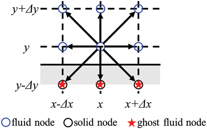
Figure 1: Schematic of lattice nodes for ghost fluid layer constructed on the solid wall

However, implementation of the contact angle schemes in the pseudopotential LB model was demonstrated to bring about many unphysical or inaccurate simulation results in the past. Spurious current is a common problem in simulating multiphase flow in LBM, which mostly occurs adjacent to the multiphase interface [20]. A large magnitude of spurious current may not only result in algorithm collapse but also make the real fluid flow velocity indistinguishable. It was reported [22,27] that the introduction of fluid-solid interaction force in the pseudopotential LB model enlarges the spurious current. When simulating wall wettability in the pseudopotential LB model, Hu et al. [28] found that fluid density near the wall deviates from the bulk fluid density. They pointed out that such deviation should be eliminated because it is uncontrollable, which makes the simulation results inaccurate.

To clarify the numerical accuracy and stability of different contact angle schemes in simulating static wetting and dynamic wetting phenomenon, the five widely used contact angle schemes as listed in Table 1 are applied to simulate a sessile droplet on a 2D plate solid wall and the capillary imbibition in a 2D channel in this paper as examples of static wetting and dynamic wetting respectively. Capillary imbibition in a 2D channel is a basic fluid transport mechanism in porous media, which is induced by the dynamic wetting of solid walls and has been investigated widely previously [29–32]. There are also many existing theories for capillary imbibition [5,33,34] for LB simulation results compared. The simulation results obtained by using the five contact angle schemes are compared in terms of simulated contact angle ranges for which numerically stable solutions can be obtained, magnitudes of spurious velocities, fluid density deviation near the wall in static wetting and the dynamics of the liquid-vapor interface in capillary imbibition.

2  Pseudopotential Multiphase Lattice Boltzmann Model

The fluid flow dynamics are governed by the macroscopic continuity equation and the Navier-Stokes equation as follows:

∂ρ∂t+∇⋅(ρU)=0(1)

∂(ρU)∂t+∇⋅(ρUU)=−∇p+∇⋅[ρυ(∇U+(∇U)T)]+F(2)

where ρ is the fluid density, U is the fluid flow velocity, p is pressure, υ is the kinetic viscosity and F is the force term. In the LBM, the fluid dynamics are described by the evolution of microfluid particles density distribution functions fi(x,t). The evolution of fluid density distribution function fi(x,t) with LBGK collision operator [35] is governed by the following equation so that the macroscopic equation of Eqs. (1) and (2) can be recovered:

fi(x+eiΔt,t+Δt)−fi(x,t)=−1τ[fi(x,t)−fieq(x,t)]+Δfi(x,t)(3)

where ei is the discrete velocity, the index i is the 9 directions of discrete velocities in a 2D lattice, Δt is the time spacing equaling 1.0, τ is the dimensionless relaxation time, fieq(x, t) is the equilibrium density distribution, and Δfi(x,t) is the force term. The equilibrium density distribution function fieq(x, t) in Eq. (3) is given as:

fieq(x,t)=ρωi[1+ei⋅ucs2+(ei⋅u)22cs4−u⋅u2cs2](4)

where ωi is the weighting coefficient, cs is sound speed in lattice unit equaling 1/3, and u is the equilibrium velocity of fluid particles. The discrete velocities ei and weighting coefficient ωi are expressed as follows:

ei={(0,0),i=0c(cos⁡π(i−1)2,sin⁡π(i−1)2),i=1,2,3,42c(cos⁡π(2i−9)4,sin⁡π(2i−9)4),i=5,6,7,8(5)

ωi={4/9,i=01/9,i=1,2,3,41/36,i=5,6,7,8(6)

c is the lattice speed which is given by c = Δx/Δt=Δy/Δt, with lattice spacing Δx=Δy=1. The macro fluid density ρ and equilibrium velocity of fluid particles u are calculated as follows:

ρ(x,t)=∑ifi(x,t)(7)

u(x,t)=∑ifi(x,t)eiρ(x,t)(8)

In this study, the internal forces or external forces are incorporated into Eq. (3) by the exact difference method [36] so that Δfi(x,t) is given as follows:

Δfi(x,t)=fieq[ρ(x,t),u(x,t)+Δu]−fieq[ρ(x,t),u(x,t)](9)

where Δu=F⋅Δt/ρ is the velocity change due to force F on fluid particles. F=Fint+Fads, where Fint is the fluid-fluid interaction force among fluid particles and Fads is the fluid-solid interaction force between bulk fluid and solid wall. The real macro velocity of fluid particles U should be then calculated as:

U(x,t)=∑ifi(x,t)eiρ(x,t)+ΔtF(x,t)2ρ(x,t)(10)

The kinetic viscosity υ in bulk fluid and at the liquid-vapor interface are given as:

υ=(τ−1/2)cs2Δt(11)

υ=υliquid⋅ρ−ρvaporρliquid−ρvapor+υvapor⋅ρliquid−ρρliquid−ρvapor(12)

In Shan-Chen pseudopotential LB model, a “effective mass” at every fluid node is introduced to mimic interaction forces among fluid particles (Fint) [19]. In this study, the fluid-fluid interaction force Fint is calculated following the force approximation approach given by Kupershtokh et al. [37] as:

Fint(x)=−βψ(x)∑x′G(x,x′)ψ(x′)(x′−x)−1−β2∑x′G(x,x′)ψ2(x′)(x′−x)(13)

where G(x,x′) is the Green function, which satisfies G(x,x′)=G(x′,x). ψ(x) is the effective mass of a fluid node, and its form is given by Yuan et al. [38] as follows:

ψ(x)=2(pEOS−ρcs2)c0g(14)

where c0=6.0 and g is a parameter only required to be ensured that the whole term in the square root is positive. pEOS is the pressure which can be obtained from a given equation of state (EOS). P-R EOS is used in this study to calculate pEOS as follows:

p=ρRT1−bρ−aρ2ε(T)1+2bρ−b2ρ2(15a)

b=0.0778RTc/pc,a=0.4572R2Tc2/pc(15b)

ε(T)=[1+(0.3746+1.5423ω−0.2699ω2)(1−T/Tc)]2(15c)

where Tc and pc are critical temperature and critical pressure, respectively. The acentric factor ω for water is 0.344, a = 2/49, b = 2/21 and R = 1 [38]. If the P-R EOS is used in the simulation, β=1.16 in Eq. (13) as given by Gong et al. [39].

3  Results and Discussions

3.1 A 2D Sessile Droplet on a Plate Wall Simulated by Different Contact Angle Schemes

The static wetting of a 2D sessile droplet on a plate solid wall is simulated by using different contact angle schemes in the following sections. The schematic of a 2D sessile droplet on a plate solid wall is shown in Fig. 2, with the simulation domain NX×NY=500×200 and the thickness of a plate solid wall Hsub=20. Periodic boundary conditions are applied at the left and right of the simulation domain, while non-slip wall boundary conditions are applied at the top of the simulation domain as well as at the plate solid wall. A 2D semi-circle droplet is initialized on the plate solid wall with initial radius R0=50, and different contact angle schemes are applied at the plate solid wall to simulate wetting phenomenon. The liquid density and vapor density are initialized as the saturated densities of the system temperature (ρsat,l=5.9 and ρsat,v=0.58 for 0.9Tc; ρsat,l=7.2 and ρsat,v=0.2 for 0.8Tc) in lattice units. The kinetic viscosities of liquid and vapor are set as 0.17 and 2.08. With the evolution of simulation time, the droplet finally reaches equilibrium status. Then, the static contact angle, spurious velocities and droplet liquid density variation near the plate solid wall can be measured. All the algorithm of the LB simulation in this study is coded by the C program language. The units of all the variables are presented in lattice units in our simulation. Conversion from lattice units to physical units is realized by using the reduced properties, with the reduced properties expressed as Tr=(Tc)real/(Tc)lu, ρr=(ρsat,l)real/(ρsat,l)lu, υr=(υsat,l)real/(υsat,l)lu, σr=(σsat)real/(σsat)lu.

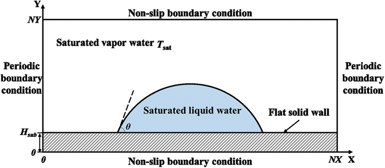
Figure 2: Schematic of a 2D sessile droplet on a plate solid wall simulated by LBM with different contact angle schemes

The four different contact angle schemes used in this paper as listed in Table 1 are described as follows:

3.1.1 Scheme #1: Pseudopotential-Based Scheme

In this contact angle scheme, the fluid-solid interaction forces Fads near the plate solid wall are given by Sukop et al. [21], which is expressed as:

Fads(x)=−Gsψ(x)∑iωis(x+ei)ei(16)

where Gs represents the fluid-solid interaction strength, and s(x + ei) is a switch function which equals to 1 for a solid node and 0 for a fluid node.

3.1.2 Scheme #2: Improved Virtual-Density Scheme

In this contact angle scheme, a virtual density ρw(x) is given to a plate solid node and the fluid-solid interaction strength can be adjusted by the virtual density. The fluid-solid interaction force Fads near wall is calculated as follows [24]:

Fads(x)=−Gsψ(x)∑iωiψ(ρw(x))s(x+ei)ei(17a)

ρw(x)={φρave(x),φ≥1,for decreasing θ compared with ρave(x)ρave(x)−Δρ,Δρ≥0,for increasing θ compared with ρave(x)(17b)

ρave=∑iωiρ(x+ei)[1−s(x+ei)]/∑iωi[1−s(x+ei)](17c)

when the virtual-density of solid wall nodes ρw(x)=ρave, the corresponding contact angle θ=90∘ as indicated by Li et al. [24]. Other contact angles can be simulated by adjusting the virtual density ρw(x) according to Eq. (17b).

3.1.3 Scheme #3: Modified Pseudopotential-Based Scheme with a Ghost Fluid Layer Constructed by Using the Fluid Density Above Wall

In this contact angle scheme, the fluid-solid interaction force Fads near wall is given by Li et al. [22], which is expressed as follows:

Fads(x)=−Gsψ2(x)∑iωis(x+ei)ei(18)

A ghost fluid layer is constructed at the plate solid wall according to Wu et al. [25]. The densities of the ghost fluid nodes on the wall are copied from nearby fluid layer, i.e., ρghost(x,y)=ρf(x,y+2), where ρghost(x,y) is the ghost fluid density at x(x, y) on a plate solid wall node and ρf(x,y+2) is the fluid density at x(x, y + 2) above the plate solid wall. The fluid-fluid interaction force Fint on the fluid node at position x(x, y + 1) can be then calculated according to Eq. (13).

3.1.4 Scheme #4: Modified Pseudopotential-Based Scheme with a Ghost Fluid Layer Constructed by Using Weighted Average Density of Surrounding Fluid Nodes

In this contact angle scheme, the fluid-solid interaction force Fads near wall is calculated following the same Eq. (18) as Scheme #3. However, the construction method of the ghost fluid layer on the plate solid wall is different from that of Scheme #3. In Scheme #4, density of the ghost fluid node constructed on the wall equals to the weighted average density of the surrounding fluid nodes as proposed by Yang et al. [26]. The ghost fluid node density ρghost(x) at position x(x, y) is expressed as follows:

ρghost(x)=∑iωiρ(x+eiΔt)[1−s(x+eiΔt)]/∑iωi[1−s(x+eiΔt)](19)

The fluid-fluid interaction force Fint on the fluid node at position x(x, y + 1) can be then calculated according to Eq. (13).

3.1.5 Scheme #5: Geometric Formulation Scheme

In the geometric formulation scheme [23,40,41], the virtual density of a solid node is given as:

ρi,0=ρi,2+tan⁡(π/2−θpre)|ρi+1,1−ρi−1,1|(20)

where the subscript i represents the coordinate tangential to the solid wall surface, the second subscript (i.e., 0, 1, 2) represents the coordinate perpendicular to the solid wall surface. ρi+1,1, ρi−1,1 and ρi,2 represent the fluid density above the solid node at (i,0), and θpre is the prescribed contact angle. After virtual densities of the solid nodes are given according to Eq. (20), the fluid-solid interaction force can be calculated according to Eq. (13) and the prescribed contact angle is simulated.

3.2 Numerical Stability of Different Contact Angle Schemes

In this study, the fluid density ratio in simulation equals to the saturated fluid density ratio at the system temperature. If the system temperature is assigned as 0.9Tc, the corresponding density ratio is ρl,sat/ρv,sat=10; If the system temperature is assigned as 0.8Tc, the corresponding density ratio is ρl,sat/ρv,sat=36. Figs. 3a–3d show that for different contact angle schemes the simulated contact angles at different fluid density ratios are different, for the same fluid-solid interaction strength (Gs or ρw). This indicates that the simulated contact angles are not only dependent on the fluid-solid interaction strength (Gs or ρw) but also density ratio dependent, which has been also pointed out by previous studies [28]. However, with the implementation of geometric formulation contact angle scheme (Scheme #5), the simulated contact angles at different fluid density ratios are the same, equaling to the prescribed contact angles as shown in Fig. 3e. It is also noted that in Scheme #1 the simulated contact angle range for which numerically stable solutions can be obtained at density ratio of 36 is considerably smaller than that at density ratio of 10. However, in Schemes #2, #3, #4 and #5 the simulated contact angle range for which numerically stable solutions can be obtained at density ratio of 36 is nearly the same as that at density ratio of 10. This demonstrates that with the application of Scheme #2, Schemes #3, #4 or Scheme #5, the algorithm gets more stable than Scheme #1 at a large density ratio in simulating static wetting of a plate solid wall.

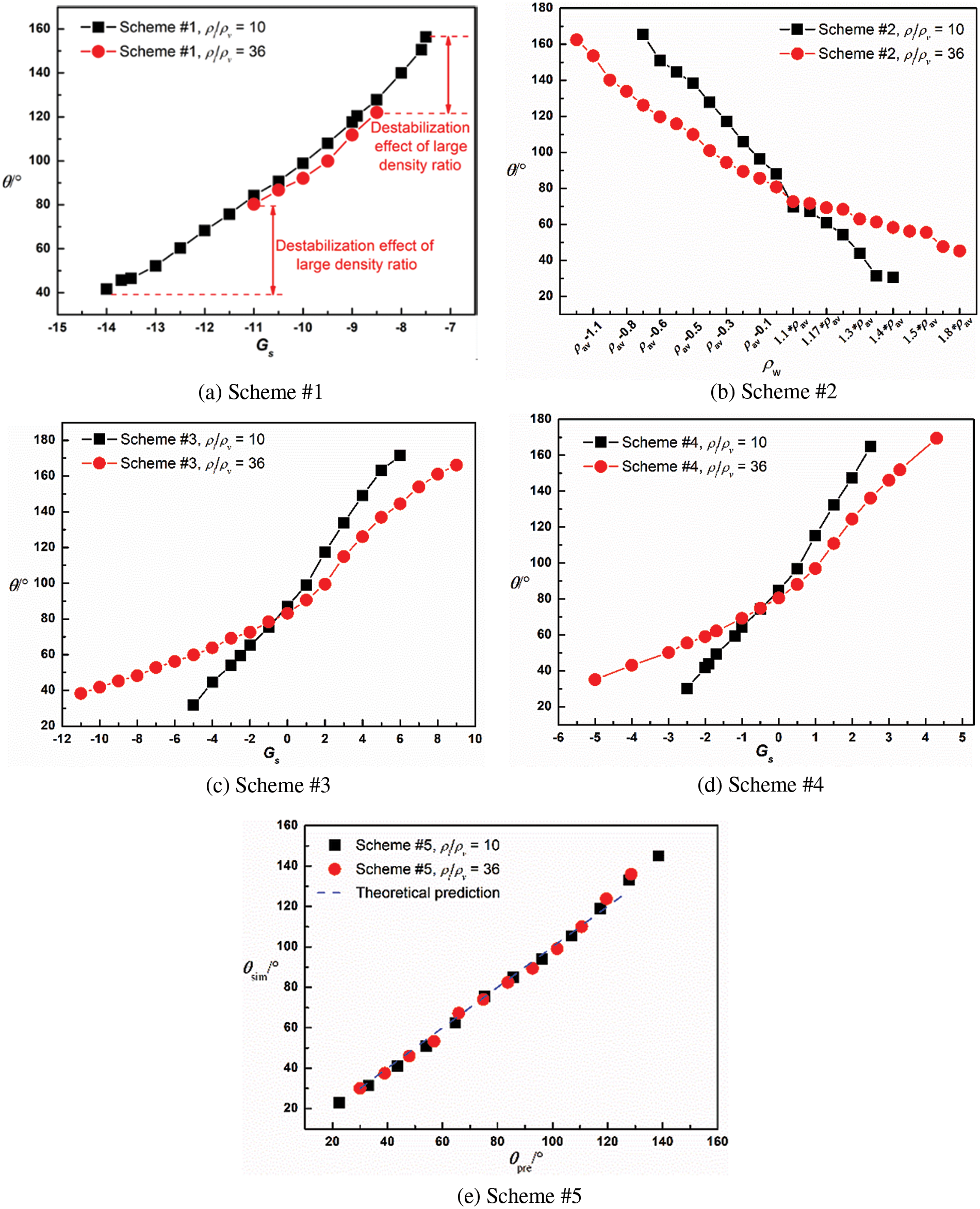
Figure 3: The static contact angles (θ) of a sessile droplet on a plate solid wall under different density ratios (ρl/ρv=10 and ρl/ρv=36) simulated by different contact angle schemes

3.3 Spurious Velocities in Simulation

The fluid flow velocities in LB simulation of a sessile droplet on a plate wall by using different contact angle schemes at two density ratios (10 and 36) are shown in Fig. 4. It can be seen that if the fluid density ratio is at 10, the fluid flow velocities are very small (the velocity magnitude is characterized by the vector length) in each contact angle scheme. The small magnitudes of fluid flow velocities in the simulation are consistent with the real fluid flow velocities, where both liquid phase and vapor phase are at stagnant status. However, if the fluid density ratio increases to 36, the fluid flow velocities magnitudes increase considerably in each contact angle scheme, especially in the ambient vapor phase. This is caused by the increased magnitudes of spurious velocities with the increasing fluid density ratio.

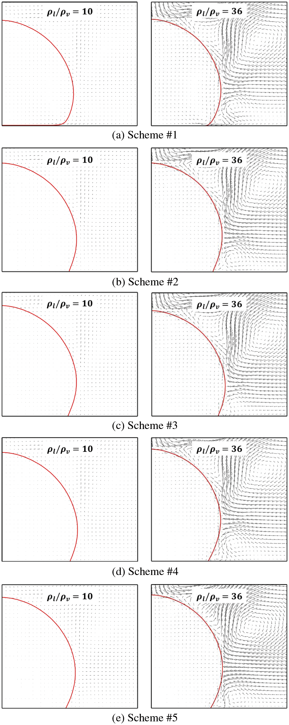
Figure 4: Velocity fields in LB simulation of a sessile droplet on a plate solid wall with contact angle θ≈120∘ at different density ratios (ρl/ρv=10 and ρl/ρv=36) obtained by using different contact angle schemes (vector length scales are the same)

Spurious velocities appear mostly adjacent to the multiphase interface, especially at the droplet triple-phase contact line. The comparison of fluid flow velocities around the triple-phase contact line of a sessile droplet on a plate solid wall simulated by Schemes #2 and #3 at the same density ratio of 10 is shown in Fig. 5. It is shown that the fluid flow velocities around the triple-phase contact line simulated by Scheme #2 are smaller than those simulated by Scheme #3 (as indicated inside the blue rectangular). This demonstrates that the Scheme #2 has smaller spurious velocities than the Scheme #3 so that it can simulate fluid flow velocities more accurately around the triple-phase contact line.

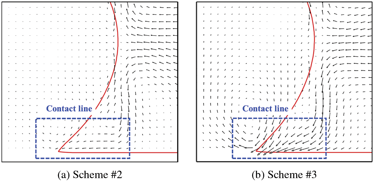
Figure 5: Comparison of fluid flow velocities around the triple-phase contact line of a sessile droplet on a plate solid wall (ρl/ρv=10, θ≈150∘) simulated by (a) Scheme #2 and (b) Scheme #3 (vector length scales are the same)

The maximum spurious velocities in LB simulation of a sessile droplet on a plate solid wall at different density ratios ρl/ρv=10 and ρl/ρv=36 by using different contact angle schemes are shown in Fig. 6. It can be seen from Fig. 6a that at low density ratio ρl/ρv=10 the maximum spurious velocities in Schemes #1, #2 and #5 are small while those in Scheme #3 are the largest for simulating any contact angles. It is also shown that the magnitudes of maximum spurious velocities in Schemes #3 and #4 are contact angle dependent. Only when the simulated contact angle in Schemes #3 and #4 is close to 90∘, the magnitudes of maximum spurious velocities are small, otherwise they are amplified. With the ghost fluid node constructed by using weighted average density of the surrounding fluid nodes (as Scheme #4), the maximum spurious velocities are smaller than those with the ghost fluid node constructed by directly using density of the fluid layer above wall (as Scheme #3). With the increased density ratio ρl/ρv=36 as shown in Fig. 6b, similar conclusions to those at low density ratio of ρl/ρv=10 can be obtained. Noted that for simulating acute contact angles at large density ratio ρl/ρv=36 the maximum spurious velocities in Schemes #1, #2, #3 and #4 become nearly the same, while they are the smallest in Scheme #5.

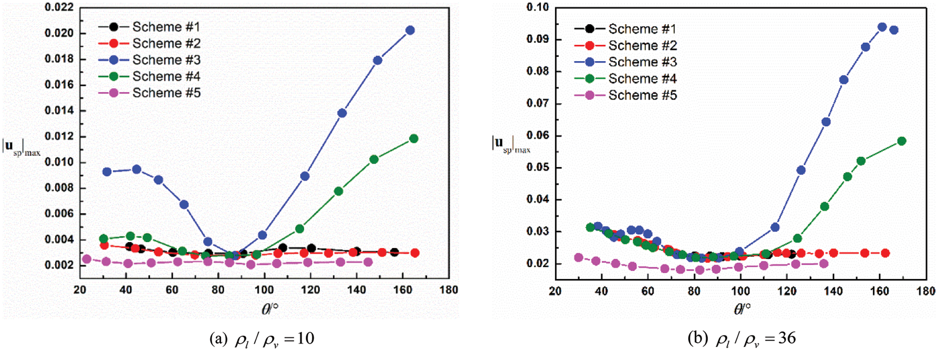
Figure 6: The maximum spurious velocities |usp|max in LB simulation of a sessile droplet on a plate solid wall at different density ratio (a) low density ratio of ρl/ρv=10 (b) high density ratio of ρl/ρv=36 by using different contact angle schemes

3.4 Fluid Density Variation Near Solid Wall

The fluid density variation near the solid wall having acute contact angle θ≈60∘ simulated by using different contact angle schemes are shown in Fig. 7. Figs. 7b and 7e show that the fluid density distribution near wall in Schemes #2 and #5 are accurate. However, Figs. 7a, 7c and 7d show that the fluid density variation near wall appears in Schemes #1, #3 and #4. In Scheme #1 (as shown in Fig. 7a) the fluid density variation appears both in the liquid phase and in the ambient vapor phase, while the fluid density variation appears only in the liquid phase in Scheme #3 and Scheme #4 as shown in Figs. 7c and 7d, respectively. This demonstrates that the inaccuracy of fluid density distribution near wall is the most significant in Scheme #1 for simulating an acute contact angle.

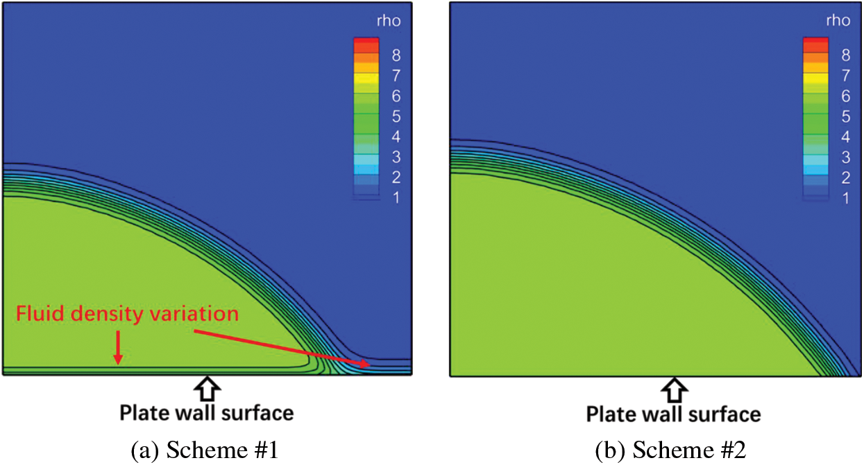
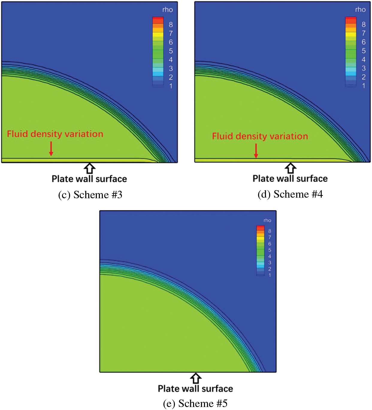
Figure 7: Fluid density distribution in LB simulation of a sessile droplet on a plate solid wall (ρl/ρv=10) with acute contact angle θ≈60∘ simulated by using different contact angle schemes

The fluid density variation near wall having obtuse contact angle θ≈120∘ simulated by using different contact angle schemes are shown in Fig. 8. Figs. 8b, 8d and 8e show that the fluid density distribution near wall by using Schemes #2, #4 and #5 are accurate, while Figs. 8a and 8c show that the fluid density variation near wall appears by using Schemes #1 and #3. It is also noted that the fluid density variation is more significant in Scheme #1 than in Scheme #3, which indicates that the inaccuracy on fluid density distribution near wall in Scheme #1 is the most significant in simulating an obtuse contact angle.

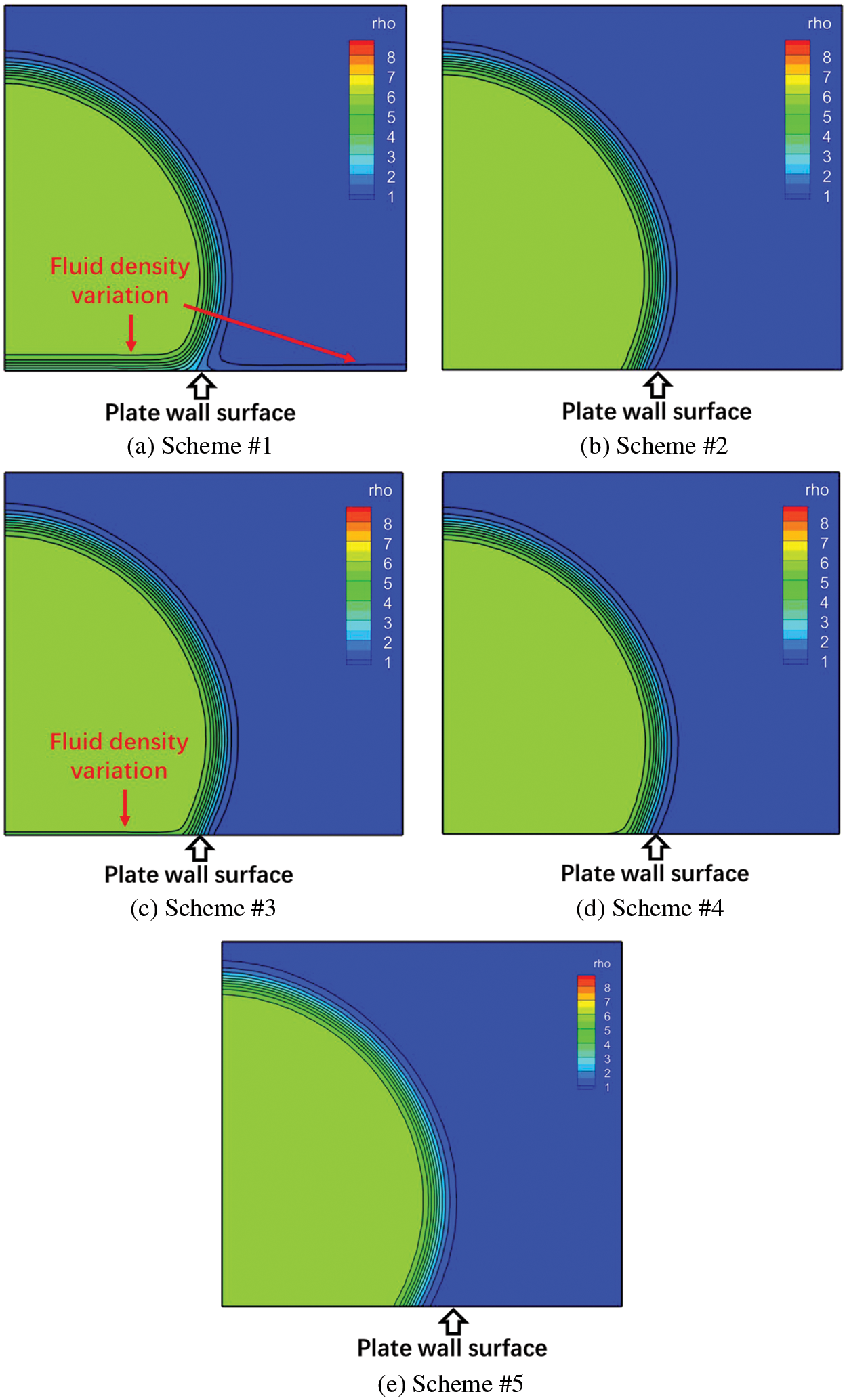
Figure 8: Fluid density distribution in LB simulation of a sessile droplet on a plate solid wall (ρl/ρv=10) with obtuse contact angle θ≈120∘ simulated by different contact angle schemes

The liquid density variations near wall (ρl/ρsat,l) in Figs. 7 and 8 are plotted vs. the perpendicular distance away from the solid wall (y) as shown in Figs. 9a and 9b, respectively. It is shown in Fig. 9a that ρl/ρsat,l=1 at any distance from the wall in Schemes #2 and #5 so that the fluid density distribution near wall is accurately simulated. However, the fluid density variation in Scheme #1 is the largest ρl/ρsat,l=0.8 at the fluid node which is nearest the solid wall, so that Scheme #1 is the most inaccurately in simulating liquid density distribution near wall. It is also noted that with the ghost fluid node constructed by using weighted average density of surrounding fluid nodes (as Scheme #4), the simulation results are more accurate than those with the ghost fluid node constructed by directly using density of the fluid layer above wall (as Scheme #3). The similar conclusions can be obtained in Fig. 9b, when simulating an obtuse contact angle of a plate solid wall by using different contact angle schemes. Noted that for simulating an obtuse contact angle the fluid density variation near wall occurs in Scheme #2, but the fluid density distribution near wall in Scheme #5 is still accurate. It is demonstrated that Scheme #5 is the most accurate contact angle scheme in terms of simulating fluid density distribution near wall.

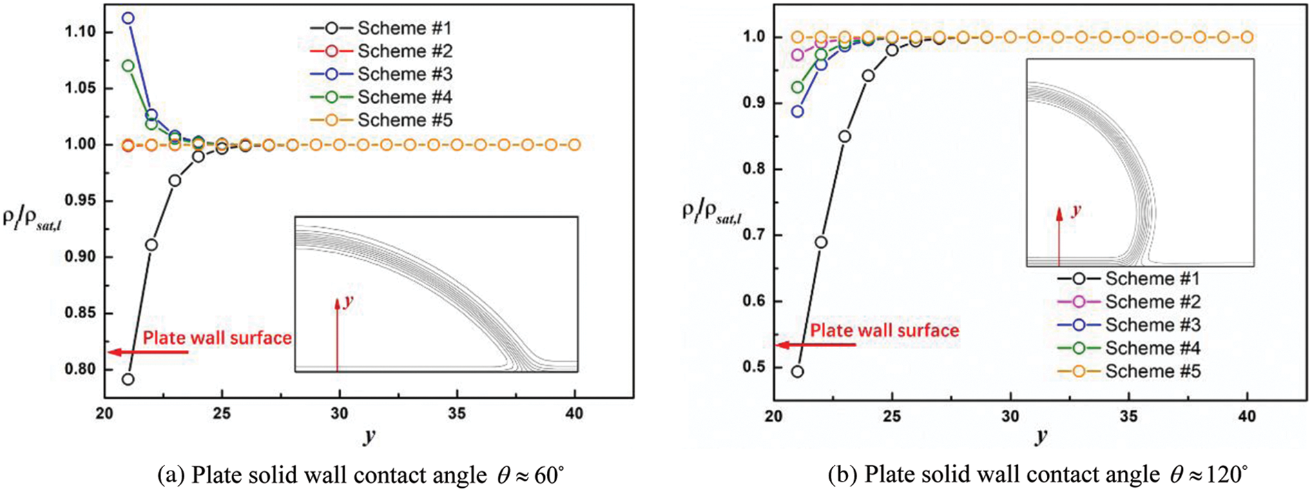
Figure 9: Liquid density variation near the plate solid wall inside a sessile droplet (ρl/ρv=10) simulated by using different contact angle schemes

3.5 Capillary Imbibition

To compare numerical accuracy of different contact angle schemes in simulating dynamic wetting of solid wall, the five widely used contact angle schemes are applied to simulate capillary imbibition in a two-dimensional (2D) channel formed by two separated parallel plates as shown in Fig. 10. Non-slip wall boundary conditions are applied at wall boundaries and periodic boundary conditions are applied at other boundaries of the simulation domain. Liquid density and vapor density are set as 5.91 and 0.58, which are the saturated densities of 0.9Tc in lattice unit. Kinetic viscosities of liquid and vapor are set as 0.17. The liquid-vapor interface moves forward in the channel with time, driven by the capillary force. It is noted that contact angle hysteresis effects are neglected in this study, in such situation the liquid-vapor interface movement follows the well-known Washburn law [33,42]:

x2(t)−x2(0)=γHcos⁡(θ)3μt(21)

where γ is the liquid-vapor surface tension, θ is the static contact angle, μ is the liquid dynamic viscosity, H is the channel height between the two separated parallel plates and the factor 3 is determined by the geometry of the channel.

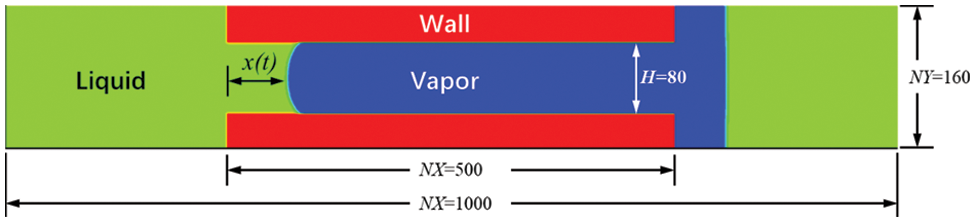
Figure 10: Schematic of 2D capillary imbibition between two parallel plates

Three groups of grids (NX×NY=1000×160, NX×NY=1200×360, NX×NY=1400×560) have been used to simulate the 2D capillary imbibition phenomenon with the application of Scheme #5 for grid independent test as shown in Fig. 11. Fig. 11 shows the liquid-vapor interface position inside the 2D channel vs. simulation time. It can be seen that the liquid-vapor interface positions x simulated by using any of the three grids are identical at any simulation time t, so that the grid NX×NY=1000×160 is chosen in present simulation to save computational resources and maintain high computational efficiency.

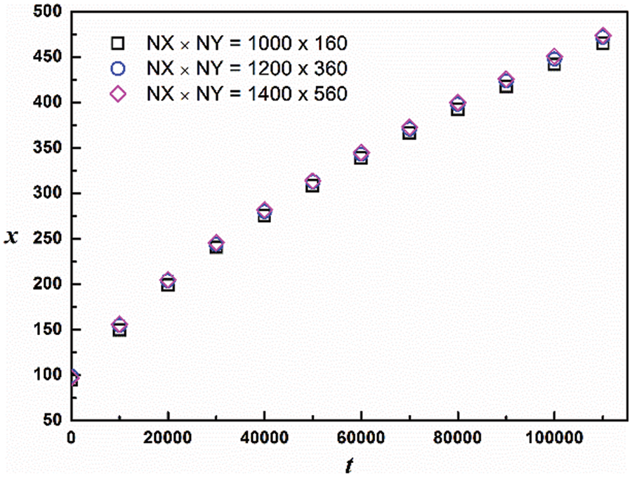
Figure 11: Grid independence test for capillary imbibition

The comparisons of LB simulation by using different contact angle schemes with the Washburn law of Eq. (21) at different wall contact angles (θ=44∘ and θ=60∘) are shown in Fig. 12. Fig. 12a shows that for θ=44∘ the LB simulation results obtained from Schemes #3, #4 and #5 agree well with the Washburn law of Eq. (21), with Scheme #5 having the most accuracy. The LB simulation results obtained from Schemes #1 and #2 deviate from the Washburn law significantly, with Scheme #1 having the least accuracy. If the wall contact angle increases to θ=60∘ as shown in Fig. 12b, the LB simulation results obtained from Schemes #3, #4 and #5 still agree well with the Washburn law of Eq. (21). The LB simulation results obtained from Scheme #2 at θ=60∘ get more closer to the Washburn law than those at θ=44∘, which means that the accuracy of Scheme #2 is increased at higher contact angles. The LB simulation results obtained from Scheme #1 at θ=60∘ still deviate from the Washburn law a lot, which demonstrates that the numerical accuracy of Scheme #1 is the lowest in simulating dynamic wetting. The large deviation of Scheme #1 is believed to be resulted from the significant fluid density variation near wall as demonstrated before in Section 3.4.

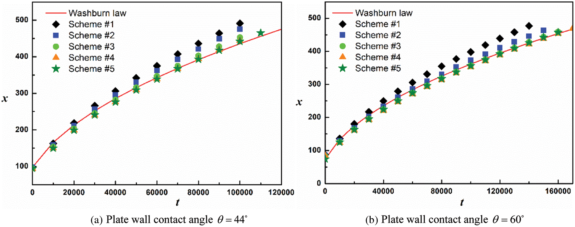
Figure 12: Liquid-vapor interface position (x) vs. time (t) at different plate wall contact angles (a) θ=44∘, (b) θ=60∘ simulated by using different contact angle schemes

4  Conclusion

Five widely used contact angle schemes based on the pseudopotential LB model are applied to simulate the problems of a 2D sessile droplet on a plate solid wall and capillary imbibition in a 2D channel, for the purpose of clarifying numerical stability and accuracy of the contact angle schemes in the simulation of static wetting and dynamic wetting. The main conclusions are summarized as follows:

1.    For contact angle schemes using fluid-solid interaction force to simulate solid wall wetting (PB scheme, IVD scheme, MPB-C scheme and MPB-W scheme) the simulated static contact angles of wall are different at different density ratios, even with the same liquid-solid interaction strength. While GF scheme simulates solid wall wetting based on geometric formulation with a prescribed contact angle, the simulated static contact angles are consistent at different density ratios.

2.    The IVD scheme, MPB-C scheme, MPB-W scheme and GF scheme are more stable than the PB scheme so that the former schemes can simulate a wide range of contact angles in static wetting simulations at large density ratios.

3.    The increased density ratio enhances spurious velocity in all the contact angle schemes, which results in the simulated fluid flow velocity in errors. The maximum spurious velocities in the GF scheme are the smallest at any density ratio so that the GF scheme is supposed to simulate fluid flow velocities more accurately.

4.    The liquid density deviation near wall in the GF scheme is the smallest, and the liquid density deviation near wall in the PB scheme is the largest. So that the thickness of the unphysical fluid density variation layer in the GF scheme is the smallest and the variation is the most significant in the PB scheme.

5.    By constructing a ghost fluid layer on wall with the average density of surrounding fluid nodes (MPB-W) rather than by directly using the fluid layer density nearest the wall (MPB-C), the spurious velocity and fluid density deviation near wall both diminish in static wetting simulation.

6.    The MPB-C scheme, MPB-W scheme and GF scheme can simulate capillary imbibition accurately, with GF scheme having the most accuracy. The IVD scheme has low accuracy in simulating capillary imbibition at low contact angle θ=44∘, but its accuracy increases at relatively large contact angle θ=60∘. The PB scheme has the lowest accuracy in simulating capillary imbibition at both contact angles of θ=44∘ and θ=60∘, so that it is not suggested to use this contact angle scheme to simulate dynamic wetting phenomenon.

Funding Statement: This study was sponsored by the National Natural Science Foundation of China under Grant No. 52206101, Shanghai Sailing Program under Grant No. 20YF1431200 and the Experiments for Space Exploration Program and the Qian Xuesen Laboratory, China Academy of Space Technology under Grant No. TKTSPY-2020-01-01.

Conflicts of Interest: The authors declare that they have no conflicts of interest to report regarding the present study.

References

1. Arzt, E., Quan, H., McMeeking, R. M., Hensel, R. (2021). Functional surface microstructures inspired by nature–from adhesion and wetting principles to sustainable new devices. Progress in Materials Science, 120, 100823. https://doi.org/10.1016/j.pmatsci.2021.100823 [Google Scholar] [CrossRef]

2. Cheng, Z., Zhang, D., Luo, X., Lai, H., Liu, Y. et al. (2021). Superwetting shape memory microstructure: Smart wetting control and practical application. Advanced Materials, 33(6), e2001718. https://doi.org/10.1002/adma.202001718 [Google Scholar] [PubMed] [CrossRef]

3. Li, M., Li, C., Blackman, B. R. K., Eduardo, S. (2021). Mimicking nature to control bio-material surface wetting and adhesion. International Materials Reviews, 67(6), 658–681. https://doi.org/10.1080/09506608.2021.1995112 [Google Scholar] [CrossRef]

4. Ding, F., Gao, M. (2021). Pore wettability for enhanced oil recovery, contaminant adsorption and oil/water separation: A review. Advances in Colloid and Interface Science, 289, 102377. https://doi.org/10.1016/j.cis.2021.102377 [Google Scholar] [PubMed] [CrossRef]

5. Cai, J., Jin, T., Kou, J., Zou, S., Xiao, J. et al. (2021). Lucas-washburn equation-based modeling of capillary-driven flow in porous systems. Langmuir: The ACS Journal of Surfaces and Colloids, 37(5), 1623–1636. https://doi.org/10.1021/acs.langmuir.0c03134 [Google Scholar] [PubMed] [CrossRef]

6. Kang, H., Lee, G. H., Jung, H., Lee, J. W., Nam, Y. (2018). Inkjet-printed biofunctional thermo-plasmonic interfaces for patterned neuromodulation. ACS Nano, 12(2), 1128–1138. https://doi.org/10.1021/acsnano.7b06617 [Google Scholar] [PubMed] [CrossRef]

7. Wang, D., Cheng, P. (2021). Nanoparticles deposition patterns in evaporating nanofluid droplets on smooth heated hydrophilic substrates: A 2D immersed boundary-lattice boltzmann simulation. International Journal of Heat and Mass Transfer, 168, 120868. https://doi.org/10.1016/j.ijheatmasstransfer.2020.120868 [Google Scholar] [CrossRef]

8. Wang, D., Cheng, P. (2023). Constructing a ghost fluid layer for implementation of contact angle schemes in multiphase pseudopotential lattice boltzmann simulations for non-isothermal phase-change heat transfer. International Journal of Heat and Mass Transfer, 201, 123618. https://doi.org/10.1016/j.ijheatmasstransfer.2022.123618 [Google Scholar] [CrossRef]

9. Stamatopoulos, C., Milionis, A., Ackerl, N., Donati, M., Leudet de la Vallee, P. et al. (2020). Droplet self-propulsion on superhydrophobic microtracks. ACS Nano, 14(10), 12895–12904. https://doi.org/10.1021/acsnano.0c03849 [Google Scholar] [PubMed] [CrossRef]

10. Gong, S., Cheng, P. (2015). Lattice boltzmann simulations for surface wettability effects in saturated pool boiling heat transfer. International Journal of Heat and Mass Transfer, 85, 635–646. https://doi.org/10.1016/j.ijheatmasstransfer.2015.02.008 [Google Scholar] [CrossRef]

11. Sun, Y., Guo, Z. (2019). Recent advances of bioinspired functional materials with specific wettability: From nature and beyond nature. Nanoscale Horizons, 4(1), 52–76. https://doi.org/10.1039/C8NH00223A [Google Scholar] [PubMed] [CrossRef]

12. Zhang, L., Chen, L., Hu, R., Cai, J. (2022). Subsurface multiphase reactive flow in geologic CO2 storage: Key impact factors and characterization approaches. Advances in Geo-Energy Research, 6(3), 179–180. https://doi.org/10.46690/ager.2022.03.01 [Google Scholar] [CrossRef]

13. Li, Q., Luo, K. H., Kang, Q. J., He, Y. L., Chen, Q. et al. (2016). Lattice boltzmann methods for multiphase flow and phase-change heat transfer. Progress in Energy and Combustion Science, 52, 62–105. https://doi.org/10.1016/j.pecs.2015.10.001 [Google Scholar] [CrossRef]

14. Wang, H., Yuan, X., Liang, H., Chai, Z., Shi, B. (2019). A brief review of the phase-field-based lattice boltzmann method for multiphase flows. Capillarity, 2(3), 33–52. https://doi.org/10.26804/capi.2019.03.02 [Google Scholar] [CrossRef]

15. Diao, Z., Li, S., Liu, W., Liu, H., Xia, Q. (2021). Numerical study of the effect of tortuosity and mixed wettability on spontaneous imbibition in heterogeneous porous media. Capillarity, 4(3), 50–62. https://doi.org/10.46690/capi.2021.03.02 [Google Scholar] [CrossRef]

16. Wang, D., Cheng, P. (2020). Effects of nanoparticles’ wettability on vapor bubble coalescence in saturated pool boiling of nanofluids: A lattice boltzmann simulation. International Journal of Heat and Mass Transfer, 154, 119669. https://doi.org/10.1016/j.ijheatmasstransfer.2020.119669 [Google Scholar] [CrossRef]

17. Wang, D. (2022). Effects of fluid-solid wall heat transfer on the achievable simulated solid wall contact angles in pseudopotential lattice boltzmann method with different ghost fluid layers constructed at a solid wall. Heat Transfer Research, 53(8). https://doi.org/10.1615/HeatTransRes.2021040253 [Google Scholar] [CrossRef]

18. Zhu, G., Li, A. (2020). Interfacial dynamics with soluble surfactants: A phase-field two-phase flow model with variable densities. Advances in Geo-Energy Research, 4(1), 86–98. https://doi.org/10.26804/ager.2020.01.08 [Google Scholar] [CrossRef]

19. Shan, X., Chen, H. (1993). Lattice boltzmann model for simulating flows with multiple phases and components. Physical Review E, 47(3), 1815–1819. https://doi.org/10.1103/PhysRevE.47.1815 [Google Scholar] [PubMed] [CrossRef]

20. Chen, L., Kang, Q., Mu, Y., He, Y. L., Tao, W. Q. (2014). A critical review of the pseudopotential multiphase lattice boltzmann model: Methods and applications. International Journal of Heat and Mass Transfer, 76, 210–236. https://doi.org/10.1016/j.ijheatmasstransfer.2014.04.032 [Google Scholar] [CrossRef]

21. Sukop, M. C., Thorne, D. T. (2006). Lattice boltzmann modeling: An introduction for geoscientists and engineers. Berlin Heidelberg: Springer-Verlag. [Google Scholar]

22. Li, Q., Luo, K. H., Kang, Q. J., Chen, Q. (2014). Contact angles in the pseudopotential lattice boltzmann modeling of wetting. Physical Review E: Statistical, Nonlinear, and Soft Matter Physics, 90(5–1), 053301. https://doi.org/10.1103/PhysRevE.90.053301 [Google Scholar] [PubMed] [CrossRef]

23. Ding, H., Spelt, P. D. (2007). Wetting condition in diffuse interface simulations of contact line motion. Physical Review E: Statistical, Nonlinear, and Soft Matter Physics, 75, 046708. https://doi.org/10.1103/PhysRevE.75.046708 [Google Scholar] [PubMed] [CrossRef]

24. Li, Q., Yu, Y., Luo, K. H. (2019). Implementation of contact angles in pseudopotential lattice boltzmann simulations with curved boundaries. Physical Review E, 100(5–1), 053313. https://doi.org/10.1103/PhysRevE.100.053313 [Google Scholar] [PubMed] [CrossRef]

25. Wu, S., Chen, Y., Chen, L. Q. (2020). Three-dimensional pseudopotential lattice boltzmann model for multiphase flows at high density ratio. Physical Review E, 102(5–1), 053308. https://doi.org/10.1103/PhysRevE.102.053308 [Google Scholar] [PubMed] [CrossRef]

26. Yang, J., Fei, L., Zhang, X., Ma, X., Luo, K. H. et al. (2021). Improved pseudopotential lattice boltzmann model for liquid water transport inside gas diffusion layers. International Journal of Hydrogen Energy, 46(29), 15938–15950. https://doi.org/10.1016/j.ijhydene.2021.02.067 [Google Scholar] [CrossRef]

27. Khajepor, S., Cui, J., Dewar, M., Chen, B. (2019). A study of wall boundary conditions in pseudopotential lattice boltzmann models. Computers & Fluids, 193, 103896. https://doi.org/10.1016/j.compfluid.2018.05.011 [Google Scholar] [CrossRef]

28. Hu, A., Li, L., Uddin, R., Liu, D. (2016). Contact angle adjustment in equation-of-state-based pseudopotential model. Physical Review E, 93(5), 053307. https://doi.org/10.1103/PhysRevE.93.053307 [Google Scholar] [PubMed] [CrossRef]

29. Wang, D., Liu, P., Wang, J., Bao, X., Chu, H. (2019). Direct numerical simulation of capillary rise in microtubes with different cross-sections. Acta Physica Polonica A, 135(3), 532–538. https://doi.org/10.12693/APhysPolA.135.532 [Google Scholar] [CrossRef]

30. Salama, A., Cai, J., Kou, J., Sun, S., El-Amin, M. F. et al. (2021). Investigation of the dynamics of immiscible displacement of a ganglion in capillaries. Capillarity, 4(2), 31–44. https://doi.org/10.46690/capi.2021.02.02 [Google Scholar] [CrossRef]

31. Liu, Y., Berg, S., Ju, Y., Wei, W., Kou, J. et al. (2022). Systematic investigation of corner flow impact in forced imbibition. Water Resources Research, 58(10), e2022WR032402. https://doi.org/10.1029/2022WR032402 [Google Scholar] [CrossRef]

32. Tang, J., Zhang, S., Wu, H. (2022). Simulating wetting phenomenon with large density ratios based on weighted-orthogonal multiple-relaxation-time pseudopotential lattice boltzmann model. Computers & Fluids, 244, 105563. https://doi.org/10.1016/j.compfluid.2022.105563 [Google Scholar] [CrossRef]

33. Schwiebert, M. K., Leong, W. H. (1996). Underfill flow as viscous flow between parallel plates driven by capillary action. IEEE Transactions on Components, Packaging, and Manufacturing Technology: Part C, 19(2), 133–137. https://doi.org/10.1109/3476.507149 [Google Scholar] [CrossRef]

34. Shen, A., Xu, Y., Liu, Y., Cai, B., Liang, S. et al. (2018). A model for capillary rise in micro-tube restrained by a sticky layer. Results in Physics, 9, 86–90. https://doi.org/10.1016/j.rinp.2018.02.026 [Google Scholar] [CrossRef]

35. Qian, Y. H., d’Humières, D., Lallemand, P. (1992). Lattice BGK models for navier-stokes equation. Europhysics Letters, 17(6), 479. https://doi.org/10.1209/0295-5075/17/6/001 [Google Scholar] [CrossRef]

36. Kupershtokh, A. L., Medvedev, D. A. (2006). Lattice boltzmann equation method in electrohydrodynamic problems. Journal of Electrostatics, 64(7–9), 581–585. https://doi.org/10.1016/j.elstat.2005.10.012 [Google Scholar] [CrossRef]

37. Kupershtokh, A. L., Medvedev, D. A., Karpov, D. I. (2009). On equations of state in a lattice boltzmann method. Computers & Mathematics with Applications, 58(5), 965–974. https://doi.org/10.1016/j.camwa.2009.02.024 [Google Scholar] [CrossRef]

38. Yuan, P., Schaefer, L. (2006). Equations of state in a lattice boltzmann model. Physics of Fluids, 18(4), 042101. https://doi.org/10.1063/1.2187070 [Google Scholar] [CrossRef]

39. Gong, S., Cheng, P. (2012). Numerical investigation of droplet motion and coalescence by an improved lattice boltzmann model for phase transitions and multiphase flows. Computers & Fluids, 53, 93–104. https://doi.org/10.1016/j.compfluid.2011.09.013 [Google Scholar] [CrossRef]

40. Zhang, C., Zhang, H., Zhang, X., Yang, C., Cheng, P. (2021). Evaporation of a sessile droplet on flat surfaces: An axisymmetric lattice boltzmann model with consideration of contact angle hysteresis. International Journal of Heat and Mass Transfer, 178, 121577. https://doi.org/10.1016/j.ijheatmasstransfer.2021.121577 [Google Scholar] [CrossRef]

41. Qin, F., Zhao, J., Kang, Q., Derome, D., Carmeliet, J. (2021). Lattice boltzmann modeling of drying of porous media considering contact angle hysteresis. Transport in Porous Media, 140(1), 395–420. https://doi.org/10.1007/s11242-021-01644-9 [Google Scholar] [PubMed] [CrossRef]

42. Washburn, E. W. (1921). The dynamics of capillary flow. Physical Review, 17(3), 273–283. https://doi.org/10.1103/PhysRev.17.273 [Google Scholar] [CrossRef]