
 Submit a Paper
 Propose a Special lssue
 Open Access
ARTICLE

Feature Preserving Parameterization for Quadrilateral Mesh Generation Based on Ricci Flow and Cross Field
1 International School of Information Science and Engineering, Dalian University of Technology, Dalian, 116000, China
2 School of Mathematical Sciences, Dalian University of Technology, Dalian, 116000, China
3 School of Software Technology, Dalian University of Technology, Dalian, 116000, China
* Corresponding Author: Xiaopeng Zheng. Email:
(This article belongs to the Special Issue: Integration of Geometric Modeling and Numerical Simulation)
Computer Modeling in Engineering & Sciences 2023, 137(1), 843-857. https://doi.org/10.32604/cmes.2023.027296
Received 24 October 2022; Accepted 05 January 2023; Issue published 23 April 2023
 View Full Text
 Download PDF
Abstract
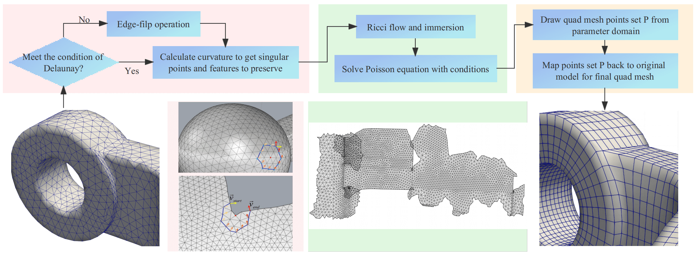
We propose a new method to generate surface quadrilateral mesh by calculating a globally defined parameterization with feature constraints. In the field of quadrilateral generation with features, the cross field methods are well-known because of their superior performance in feature preservation. The methods based on metrics are popular due to their sound theoretical basis, especially the Ricci flow algorithm. The cross field methods’ major part, the Poisson equation, is challenging to solve in three dimensions directly. When it comes to cases with a large number of elements, the computational costs are expensive while the methods based on metrics are on the contrary. In addition, an appropriate initial value plays a positive role in the solution of the Poisson equation, and this initial value can be obtained from the Ricci flow algorithm. So we combine the methods based on metric with the cross field methods. We use the discrete dynamic Ricci flow algorithm to generate an initial value for the Poisson equation, which speeds up the solution of the equation and ensures the convergence of the computation. Numerical experiments show that our method is effective in generating a quadrilateral mesh for models with features, and the quality of the quadrilateral mesh is reliable.Graphic Abstract
Keywords
The finite element method has become one of the most effective numerical analysis methods in computer graphics and industrial fields. Geometric models need to be described in the computer first so as to further modeling, analysis and simulation. The main task of the finite element method is to construct a discrete finite element mesh that accurately describes the geometric shape of the 3D model. The quality of the finite element mesh will affect the results of numerical calculation directly, so constructing a high-quality discrete finite element mesh is an important part. There are many methods to represent surfaces in the computer field, such as spline function, implicit surface, point cloud and polygon mesh. The most commonly used meshes are triangle meshes. Although triangle meshes are simple and flexible, the quadrilateral mesh elements can naturally align with the feature edges and the geometric features, such as the principal curvature direction and feature lines on surfaces. In addition, quadrilateral meshes perform well in computational accuracy and efficiency. Therefore, it has become more and more necessary to study quadrilateral mesh generation algorithms. At the same time, with the rapid development of CAE, the demands for modeling industrial models are rapidly rising, which requires higher feature preservation. A robust feature-preserving quadrilateral mesh generation algorithm is expected gradually.
Singularities are significant in quadrilateral mesh generation. In short, in quadrilateral meshes, if the number of faces around an inner vertex is not equal to 4 or the number of faces around a boundary vertex is not equal to 2, such vertices are called singular points. The number and position of singular points are crucial in quadrilateral mesh generation. But the existence of singular points is almost inevitable for complex models, especially where geometric characteristics are involved. Singularities are also related to the models’ genus and boundary number. This shows that the quadrilateral mesh generation still faces many challenges at present. Because of the important role quadrilateral meshes play in industrial software, researches on quadrilateral mesh generation are very popular at home and abroad. Many methods have been proposed for generating quadrilateral meshes, mainly including the methods based on metric [1,2], paving methods [3,4], block methods [5,6], Q-Morph methods [7], Morse theory based methods [8,9], the method combined with cross field [10,11], etc.
The Q-Morph method is stable and widely used, but its efficiency depends on the quality of the triangular mesh input. In order to generate a full quadrilateral mesh, a few elements of poor quality may be generated. The block method first computes an initial skeleton map based on the triangular mesh input. This map can roughly divide the mesh into several topological quadrilateral blocks. There are also methods [12–14] that deform the input surface into a polycube shape, which is a union of cubes, then the faces of the polycube decide the blocks. Then calculate the parameter domains of each block, and subdivide them in the parameter domain space to obtain a quadrilateral mesh. The clustering method generates the skeleton by merging the adjacent triangular surfaces into patches, such as the normal based and center based methods [5]. The paving method is based on the front advancing idea [6], and starts from the boundary of the region and advances in rows to generate quadrilateral elements. The generated mesh has good edge trimming character, but the algorithm is complex and the elements may collide.
Cross field based method has been widely studied recently. The methods based on field theory have been proposed successively to characterize the geometric features with field distribution. Each approach should choose a way to represent a cross first, for example, N-RoSy representation [11], period jump technique [15] and complex value representation [16]. Then these approaches usually generate a smooth cross field on the surface by energy minimization technique. The typical measure of field smoothness is a discrete version of the Dirichlet energy [17]. Based on the obtained cross field, realize the automatic region decomposition by analyzing the singularity of the field, using streamline tracing techniques [16] or parameterization methods [18] to generate quadrilateral mesh. Combining harmonic orthogonal field and Ginzburg-Landau theory, this work [19] realized quadrilateral mesh generation for zero genus surface. According to Ginzburg-Landau theory, this work [20] first calculates an orthogonal field, obtains a global parameterization through the orthogonal field, and then extracts quadrilateral meshes. Furthermore, there are methods [21] that construct a graph based on the structure of the smooth frame field first, and then generate a globally optimal quadrilateral skeleton graph by solving the constrained minimum weight matching problem. The characteristic of these methods is that the direction and size of quadrilateral elements are controlled by orthogonal fields on the surface. When the designed cross field is smooth enough, the generated quadrilateral grid streamline is also smooth.
Metric based method is also a popular method. This method uses the metric of mesh to establish a one-to-one correspondence between the points on the surface and the points on the parameter domain. The essence is to calculate an immersion of manifold on the parameter domain. Quadrilateral mesh is generated on the parameter domain first, and then reflected back to the physical space of surface [22] and generate quadrilateral mesh by globally defined parameterization. Sometimes the complex surfaces need to be decomposed into a series of simple surfaces and then combine these simple surfaces to form the final mesh of the complex surface [23], but how to decompose is also a very complex process. Metric based mesh generation method is a feasible method and strictly convergent in theory. Especially curvature flow based methods, there has been a lot of relevant theoretical and applied research [24–26] recently. This method takes low computation cost and is easy to be implemented.
However, methods based on metric usually perform badly on feature preserving. The exact singular points information is also needed to ensure the smallest area deformation of the obtained quadrilateral meshes. Cross field methods’ outstanding performance at feature preserving inspires us to combine the metric method with the cross field method, using the Ricci flow to reduce computation cost by mesh parameterization and provide a reliable, stable and convergent initial value for the Poisson equation. Because of its orthogonality, the cross field is consistent with the structured quadrilateral mesh. Singularities are also naturally included in the global cross field information. Compared with other methods that require additional representation, this is advantageous for subsequent calculation and representation. A large number of previous studies on cross field methods have made it easier to obtain the cross field which fits the characteristics and boundary constraints. We use the energy optimization method to obtain the required cross field. Since the study of the Ricci flow method, there have been a complete theoretical system and calculation methods about how to obtain the preliminary metric. Once the Ricci flow method is used to design metric, its convergence is guaranteed by Hamilton and Chow’s theorems.
Theorem 1.1.(Hamilton) [27] For a closed surface of non-positive Euler characteristic, the normalized Ricci flow will converge to a metric such that the Gaussian curvature is constant everywhere.
Theorem 1.2.(Chow) [28] For a closed surface of positive Euler characteristic, the normalized Ricci flow will converge to a metric such that the Gaussian curvature is constant everywhere. Which are the theoretical bases of calculating optimization metric. These theories prove the feasibility of our method. Getting a preliminary solution near the final solution in the solution space by the Ricci flow method reduces the subsequent calculation time. Trimming the metric according to the feature constraints is a follow-up adjustment of the approximate solution. Compared with the direct parameterized solution method, the existence of Ricci flow algorithm is positive, and the approximate solution can also speed up the Poisson equation’s calculation. The metric obtained by Ricci flow algorithm can induce a regular quadrilateral mesh with the guidance of the cross field. A Riemannian metric, fitting to the feature constraints and globally defined, can be calculated, and then the quadrilateral mesh can be generated.
Contributions This work opens a novel direction for generating quadrilateral mesh with feature constraints. This method encompasses the surface curvature, which is intrinsic, and the cross field method, which is external. The clear and concise theory makes the algorithm pipeline simple and automatic. Geometric features can be preserved well under our algorithm. We implemented this algorithm on some models and obtained high-quality feature preserving quadrilateral meshes.
The work is arranged as follows: Section 2 introduces the theoretical background; Section 3 explains the algorithm in detail and gives a simple example to illustrate the key ideas; The experimental results are shown in Section 4. Finally, the work concludes in Section 5.
2.1 Ricci Flow Conformal Structure
Ricci flow was proposed by Hamilton originally to solve low dimensional topology problems, such as poincaré conjecture and Thurston’s conjecture. Its specific form is
Hamilton first proved that Ricci flow could quickly converge to a constant curvature measure on a 3-manifold which has an initial measure with good curvature conditions. Observing its form, it is not difficult to see that Ricci flow continuously updates surfaces’ measure according to its Gaussian curvature. In fact, it is a process of heat flow diffusion and finally stabilized in a normal state, that is, a constant curvature.
In the following discussion, we use
Definition 2.1 (Discrete Riemannian Metric). A discrete metric on a triangular mesh is a function defined on the edges,
Definition 2.2 (Discrete Gauss Curvature). On a mesh, the discrete Gauss curvature function is defined on vertices,
where
We know that a low dimensional parameterization can be achieved by setting the target curvature to a constant in Ricci flow algorithm. For points that are not singular points, set their target curvature as
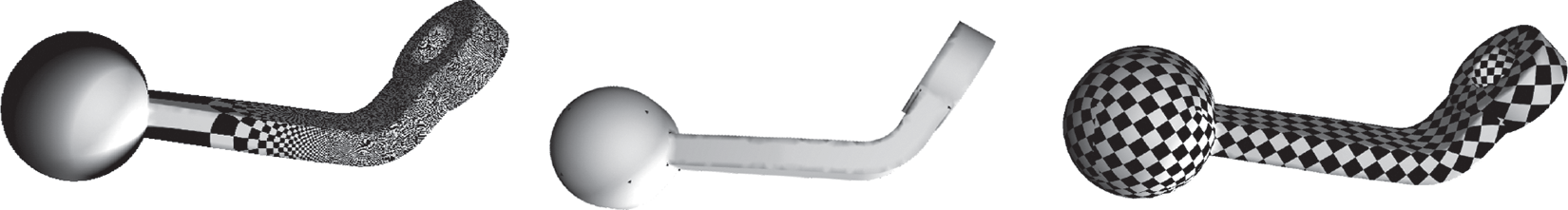
Figure 1: Huge area distortion (left), singularities (middle), slight area distortion (right)
We could obtain the canonical homology group bases which form a cut graph L of the mesh by burning method in practice. For each singularity, we find some disjoint shortest paths
2.2 Parallel Transport and Holonomy
The existence of singular points is almost inevitable, especially in complex models. We explain the influence of singular points in the combined method and how to deal with singular points from the perspective of quadrilateral mesh directly. Suppose S is a topological surface, Q is a cell partition of S, if all cells of Q are topological quadrilaterals, then (S, Q) is a quadrilateral mesh.
For a quadrilateral mesh
Definition 2.3 (Parallel Transportation). Given a quadrilateral mesh
In practice, we are more interested in the loop case, parallel transporting a tangent vector at
Definition 2.4 (Holonomy). Suppose
Because
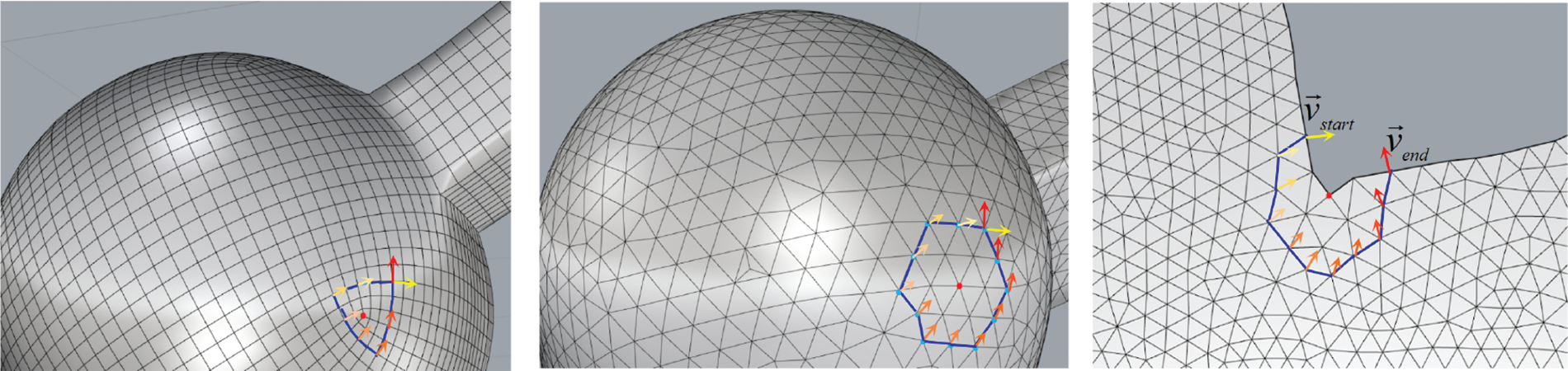
Figure 2: Discrete parallel transport and holonomy
Cross field is an important tool in various manifold operations, such as finite element subdivision, remeshing or texture mapping. A 4-symmetry direction field is defined on the tangent plane of each vertex of the surface, which is invariant by rotation of
Definition 2.5 (Cross Field). Given a smooth closed surface S,
Each face on a quadrilateral mesh is close to a square. As posted before, the internal points’ topology degree is four, which is adjacent to four faces, the topological degree of a singular point is not equal to four. Select any loop composed of faces on the quadrilateral mesh embracing a singular point, put a unit frame on the first face, the coordinate axis is parallel to the two opposite sides of the quadrilateral, and then move it to the next face in parallel. In this way, it moves parallel along the circuit until it returns to the original face. There is a rotation operation between the final frame and the initial frame, and the rotation angle is an integral multiple of
Definition 2.6 (Singularity of a Cross Field). Let
where
The next step is computing the potential function with singular information. The final parameterization should align with the given input field as well as possible, i.e., the parameterization
where F is a symmetric covering field,
Suppose the input surface S is discretized as a triangular mesh. Fig. 3 shows the algorithm chart flow. The algorithm pipeline is as follows:
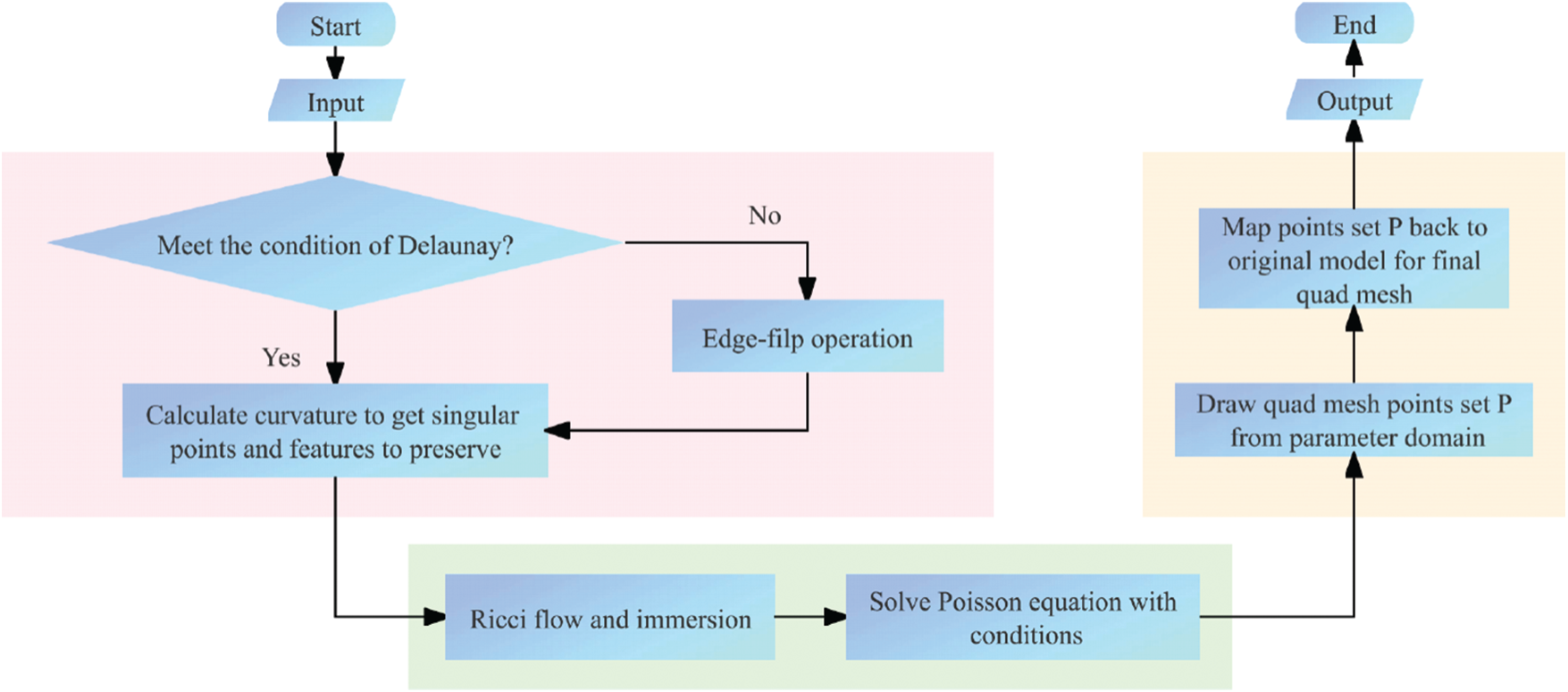
Figure 3: The algorithm flow chart
1. Calculate initial parameterization with discrete dynamic surface Ricci flow algorithm and obtain a flat metric
2. Compute a cut graph L of the surface, and some shortest paths
3. Isometrically immerse
4. Feature and boundary structure deformation. Given corresponding restrictions for feature edges and boundary edges in the Poisson equation. Such that each pair of dual boundary segments of P differs by a translation and a rotation in R. And feature edges are horizontal or vertical on the parameter plane.
5. Trace the critical graph to construct a motorcycle graph, and then the motorcycle graph induces a quadrilateral partition of surface where T-junctions are allowed. From which the final quad mesh could be generated.
In the following, we explain each step in detail.
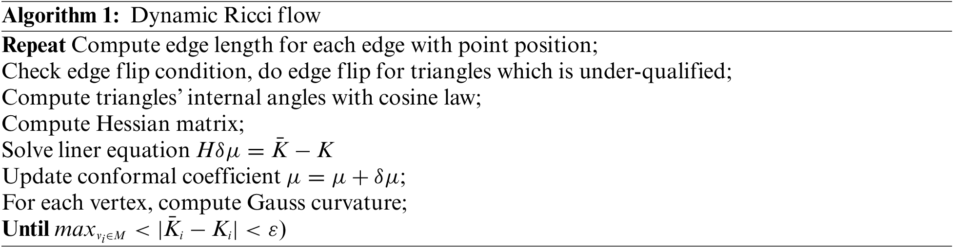
3.2 Dynamic Ricci Flow with Singularities
As mentioned above, Ricci flow is a process of metric changing under a conformal map. For each vertex
After introducing some necessary background knowledge, We can lead to the discrete Ricci energy. For a triangle
Then the discrete Ricci energy for the whole mesh is
In actual operation, the Hessian matrix is calculated with the cotangent edge weight, assume
Under the condition of regularization,
After this step, an initial metric
3.3 Compute Cut Graph and Isometric Immersion
Suppose triangle mesh M with singularities set
now
We can isometrically immerse
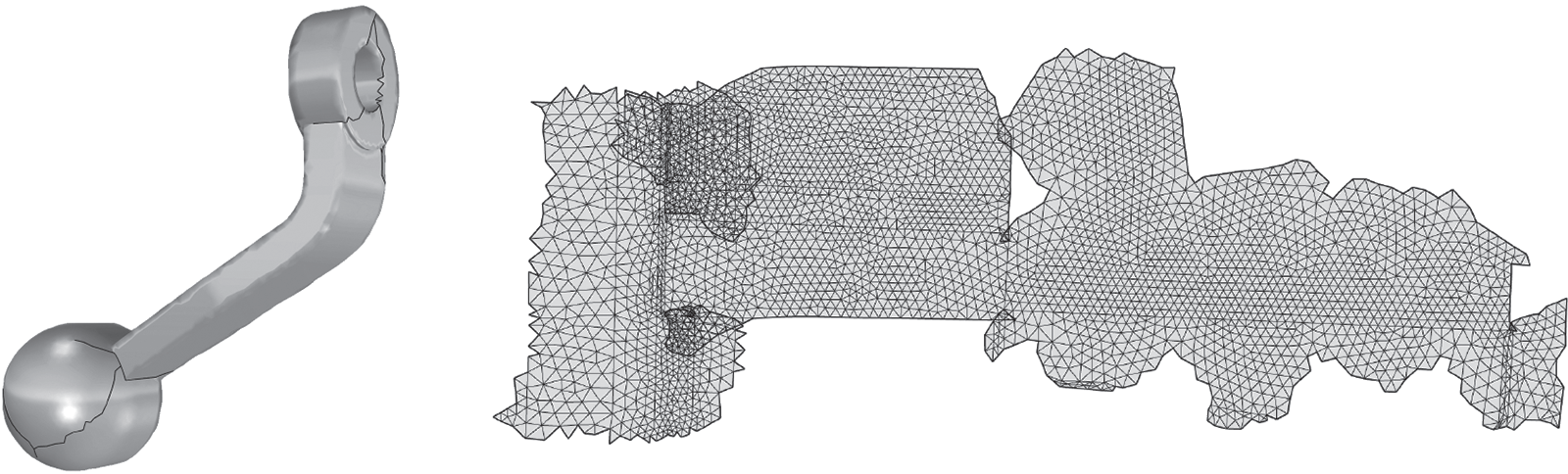
Figure 4: The shortest paths connecting singulars and boundary (left), the result of isometric immersion (right)
Like most standard cross field methods, we compute the final position distribution of points by solving a Poisson equation with constraints. Poisson equation is a partial differential equation commonly used in mathematics, electrostatics, mechanical engineering and theoretical physics. It is a non-homogeneous Laplace equation. The meaning of the equation is that the liquid flow passing through any closed surface is equal to the total amount of liquid produced by the fluid source contained in the surface. According to this character, the equation to be solved can be written as
where
This energy should be minimized.
So the final equation we have to solve can be written as:
The solution defines a parameterization on which all the feature conditions are satisfied. It is worth noting that after the parameterization of Ricci flow algorithm, the solution space of the Poisson equation is
In order to generate a seamless quadrilateral mesh, we also need to set the boundary holonomy conditions. Since we have set the target curvature at singular points in the Ricci flow algorithm, the holonomy conditions have been satisfied near the singular points. In fact, we have almost obtained an initial metric that globally satisfies the holonomy conditions. So we only need to set the boundary conditions and adjust the metric slightly to achieve our goal.
Let
We can modify the metric of mesh to achieve the holonomy conditions, such that all pairs of edges are vertical or vertical. Setting the boundary conditions, then we could calculate the coordinates of the interior vertices of
A seamless parameterization globally defined gives a quartic differential on a surface [32]. According to the singularities extract from the cross field and the metric from the Poisson equation, We trace the critical graph to construct motorcycle graph [33], shown in Fig. 5. That is the trajectories aligned parameterization axes radiate outward from the singularities until they intersect at another trajectory. Motorcycle graph induces a quadrilateral partition of the surface where T-junctions are allowed. Then, based on deck transformation conditions [34], adjust the arc length of the motorcycle graph so that the singularities are located at the rational grid points, and then optimize the global metric to be compatible with quad-mesh generation. Flatting the triangles according to the new metric to obtain a finite trajectories parameterization. The quad-mesh can be generated by sampling lattice points and pulling them back to the original surface.
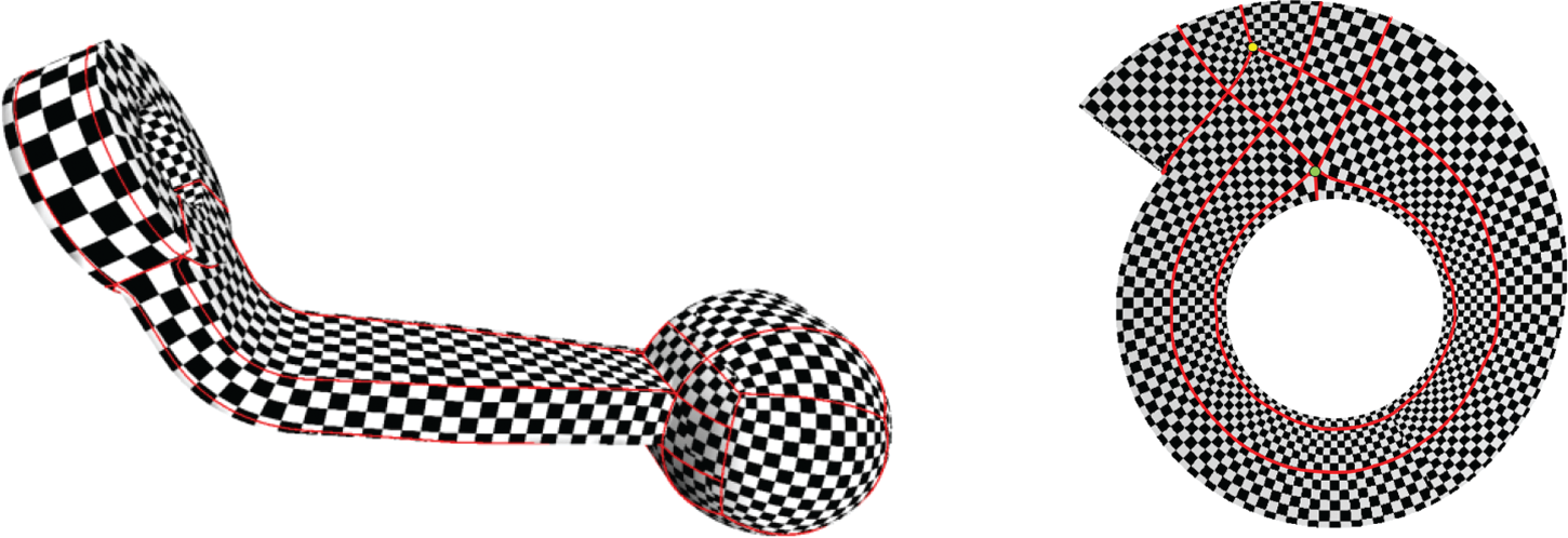
Figure 5: Final metric and motorcycle graph
In this section, we give some examples and results. All the experiments were conducted on a server with 2.10 GHz Intel(R) Xeon(R) Silver 4110 CPU, 128G RAM, GeForce RTX 2080Ti with 11G RAM and 64-bit Ubuntu operating system. The running time is reported in Table 1.

In Fig. 6, we show two models whose feature lines are complex in
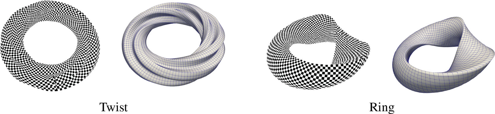
Figure 6: Final metric and quad mesh got from it
Figs. 7 and 8 illustrate the quad-meshes obtained by the proposed method. It performs well near the singular points. As can be seen from the detail box on the right side of the figure, the sharp edges around the two singular points are well preserved.
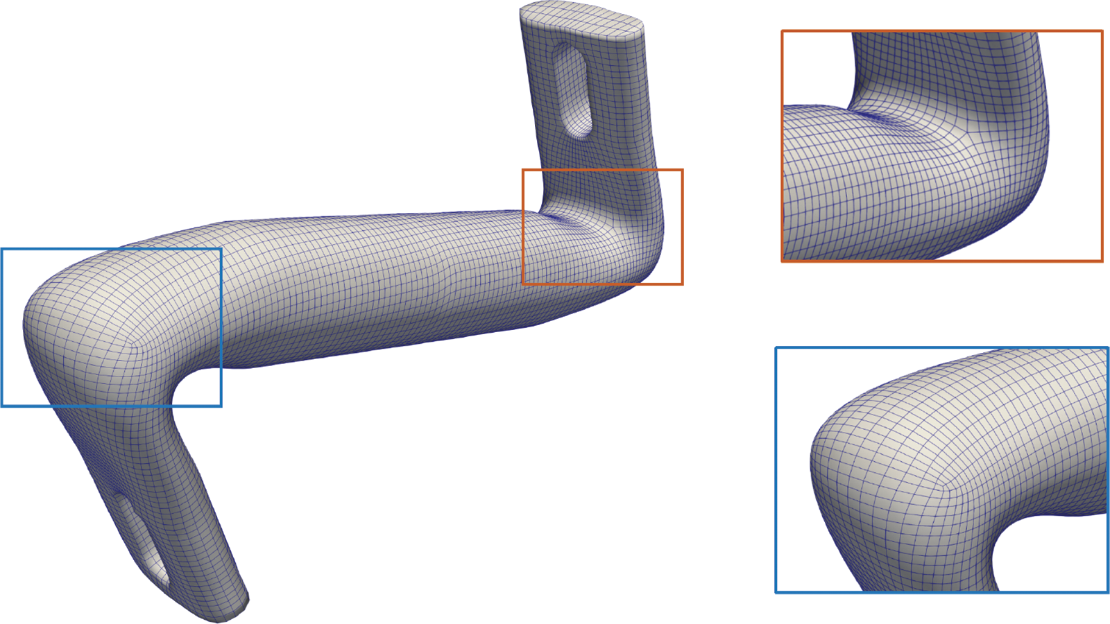
Figure 7: Quad mesh and some details (Elbow)
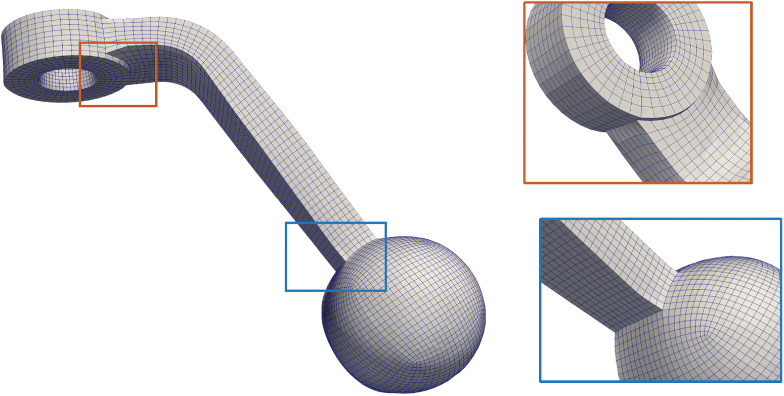
Figure 8: Quad mesh and some details (Hemisphere)
Table 1 shows the running time and data size of the models. The “Mesh Size” column contains the number of cells of the triangulation and the final quadrilateral mesh. The ‘Time’ column lists the time spent on each step of our algorithm. It can be seen that the time for Ricci flow is similar when the model size is similar. The time of solving the final metric is related to the number of feature constraints. More constraints require more iterations during the optimization process, that is, more time. Finally, when two models have almost the same level of size, the time required to generate quadrilateral mesh is also much the same. Fig. 9 shows the convergence process of the residual values with iteration steps and CPU time during the calculation process. We observe the convergence rate from two perspectives, the x axis of the blue line is CPU time, the x axis of the red line is the number of iterations, and the y axis is the residual values. It can be seen that the difference between the residual values of the two recording methods is tiny, indicating the numerical stability of the calculation and the steady convergence of the algorithm.
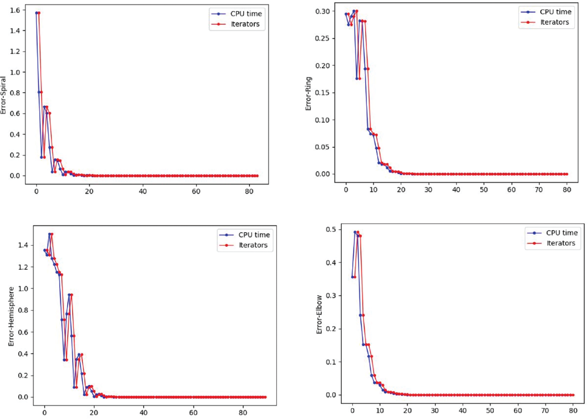
Figure 9: Residual value with iterations and CPU time
Compared to other field methods, our method performs well in computational efficiency because the Ricci flow algorithm provides a pretty good initial value for Poisson equation and greatly reduces the calculation cost through parameterization. With this initial value, there is little possibility of divergence during the optimization process. The Ricci flow algorithm reduces the dimension of computation, making our method more friendly to large models. In addition, due to the conformal property of the Ricci flow algorithm, our algorithm performs well in mesh quality.
For the models with very high genus, the Ricci flow algorithm still can be calculated, but in this case, surfaces are embedded into the Poincaré disk. The metric near the disk boundary is very small and its tiny value will always cause decisive errors in the 2D field mapping calculation, even if the embedding is translated to the middle area of the Poincaré disk by M
In this work, a new quadrilateral mesh generation algorithm is proposed based on the methods of metric and cross field. After the process of the discrete Ricci flow algorithm, a preliminary metric satisfying singularity condition is obtained, which provides a stable, convergence initial value and a low dimensional solution space for the Poisson equation. With the constraints of specific features, we solve the Poisson equation to attain the final metric. The existence and uniqueness of the solution can be ensured by the prior result of the Ricci flow algorithm. Our experimental results demonstrate the efficiency and effectiveness of the algorithm. Further work should focus on the combination of the Ricci flow and cross field methods for hexahedral mesh generation.
Funding Statement: This work is supported by NSFC Nos. 61907005, 61720106005, 61936002, 62272080.
Conflicts of Interest: The authors declare that they have no conflicts of interest to report regarding the present study.
References
1. Lai, Y. K., Jin, M., Xie, X., He, Y., Palacios, J. et al. (2009). Metric-driven rosy field design and remeshing. IEEE Transactions on Visualization and Computer Graphics, 16(1), 95–108. [Google Scholar]
2. Chen, W., Zheng, X., Ke, J., Lei, N., Luo, Z. et al. (2019). Quadrilateral mesh generation I: Metric based method. Computer Methods in Applied Mechanics and Engineering, 356, 652–668. https://doi.org/10.1016/j.cma.2019.07.023 [Google Scholar] [CrossRef]
3. Blacker, T. D., Stephenson, M. B. (1991). Paving: A new approach to automated quadrilateral mesh generation. International Journal for Numerical Methods in Engineering, 32(4), 811–847. [Google Scholar]
4. Cass, R. J., Benzley, S. E., Meyers, R. J., Blacker, T. D. (1996). Generalized 3-D paving: An automated quadrilateral surface mesh generation algorithm. International Journal for Numerical Methods in Engineering, 39(9), 1475–1489. [Google Scholar]
5. Boier-Martin, I., Rushmeier, H., Jin, J. (2004). Parameterization of triangle meshes over quadrilateral domains. Proceedings of the 2004 Eurographics/ACM SIGGRAPHSymposium on Geometry Processing, pp. 193–203. Nice, France. [Google Scholar]
6. Carr, N. A., Hoberock, J., Crane, K., Hart, J. C. (2006). Rectangular multi-chart geometry images. Proceedings of the Fourth Eurographics Symposium on Geometry Processin, pp. 181–190. Cagliari, Sardinia, Italy. [Google Scholar]
7. Owen, S. J., Staten, M. L., Canann, S. A., Saigal, S. (1998). Advancing front quadrilateral meshing using triangle transformations. Proceedings of International Meshing Roundtable, pp. 409–428. Dearborn Michiga. [Google Scholar]
8. Dong, S., Bremer, P., Garland, M., Pascucci, V., Hart, J. (2006). Spectral surface quadrangulation. ACM Transactions on Graphics, 25(3), 1057–1066. https://doi.org/10.1145/1141911.1141993 [Google Scholar] [CrossRef]
9. Jin, H., Zhang, M., Jin, M., Liu, X., Kobbelt, L. et al. (2008). Spectral quadrangulation with orientation and alignment control. ACM Transactions on Graphics, 27(5), 147. [Google Scholar]
10. Kälberer, F., Nieser, M., Polthier, K. (2007). Quadcover-surface parameterization using branched coverings, vol. 26, pp. 375–384. Berlin, Germany. [Google Scholar]
11. Palacios, J., Zhang, E. (2007). Rotational symmetry field design on surfaces. ACM Transactions on Graphics, 26(3), 55–es. https://doi.org/10.1145/1276377.1276446 [Google Scholar] [CrossRef]
12. Xia, J., Garcia, I., He, Y., Xin, S. Q., Patow, G. (2011). Editable polycube map for GPU-based subdivision surfaces. Symposium on Interactive 3D Graphics & Games, vol. 151. San Francisco, CA, USA. [Google Scholar]
13. Ying, H., Wang, H., Fu, C. W., Hong, Q. (2009). A divide-and-conquer approach for automatic polycube map construction. Computers & Graphics, 33(3), 369–380. https://doi.org/10.1016/j.cag.2009.03.024 [Google Scholar] [CrossRef]
14. Lin, J., Jin, X., Fan, Z., Wang, C. (2008). Automatic polycube-maps. Proceedings of the 5th International Conference on Advances in Geometric Modeling and Processing, pp. 3–16. Hangzhou, China. [Google Scholar]
15. Li, W. -C., Vallet, B., Ray, N., Lévy, B. (2006). Representing higher-order singularities in vector fields on piecewise linear surfaces. IEEE Transactions on Visualization and Computer Graphics, 12(5), 1315–1322. https://doi.org/10.1109/TVCG.2006.173 [Google Scholar] [PubMed] [CrossRef]
16. Ray, N., Sokolov, D. (2014). Robust polylines tracing for n-symmetry direction field on triangulated surfaces. ACM Transactions on Graphics, 33(3), 1–11. https://doi.org/10.1145/2602145 [Google Scholar] [CrossRef]
17. Jiang, T., Fang, X., Huang, J., Bao, H., Tong, Y. et al. (2015). Frame field generation through metric customization. ACM Transactions on Graphics, 34(4), 1–11. https://doi.org/10.1145/2766927 [Google Scholar] [CrossRef]
18. Ebke, H. C., Campen, M., Bommes, D., Kobbelt, L. (2014). Level-of-detail quad meshing. ACM Transactions on Graphics, 33(6), 1–11. https://doi.org/10.1145/2661229.2661240 [Google Scholar] [CrossRef]
19. Viertel, R., Osting, B. (2017). An approach to quad meshing based on harmonic cross-valued maps and the ginzburg-landau theory. arXiv preprint arXiv:1708.02316. [Google Scholar]
20. Blanchi, V., Corman, T., Ray, N., Sokolov, D. (2021). Global parametrization based on ginzburg-landau functional. NumericalGeometry, Grid Generation and Scientific Computing. Cham: Springer International Publishing. [Google Scholar]
21. Razafindrazaka, F. H., Reitebuch, U., Polthier, K. (2015). Perfect matching quad layouts for manifold meshes. Proceedings of the Eurographics Symposium on Geometry Processing, SGP'15. Eurographics Association, Graz, Austria. [Google Scholar]
22. Myles, A., Zorin, D. (2012). Global parametrization by incremental flattening. ACM Transactions on Graphics, 31(4), 1–11. https://doi.org/10.1145/2185520.2185605 [Google Scholar] [CrossRef]
23. Chen, W., Zheng, X., Ke, J., Lei, N., Luo, Z. et al. (2018). Metric based quadrilateral mesh generation. arXiv preprint arXiv:1811.12604. [Google Scholar]
24. Vacaru, S. I., Bubuianu, L. (2019). Classical and quantum geometric information flows and entanglement of relativistic mechanical systems. Quantum Information Processing, 18(12), 1–30. https://doi.org/10.1007/s11128-019-2487-z [Google Scholar] [CrossRef]
25. Bobenko, A. I., Schrder, P. (2005). Discrete willmore flow. ACM Siggraph. Los Angeles, California. [Google Scholar]
26. Colding, T. H., William, I. I., Pedersen, E. K. (2015). Mean curvature flow. Bulletin of the American Mathematical Society, 52(2), 297–333. https://doi.org/10.1090/S0273-0979-2015-01468-0 [Google Scholar] [CrossRef]
27. Hamilton, R. S. (1988). The Ricci flow on surfaces. Mathematics and General Relativity, Proceedings of the AMS-IMS-SIAM Joint Summer Research Conference in the Mathematical Sciences on Mathematics in General Relativity, pp. 237–262. Santa Cruz, California. [Google Scholar]
28. Chow, B. (1991). The Ricci flow on the 2-sphere. Journal of Differential Geometry, 33(2), 325–334. https://doi.org/10.4310/jdg/1214446319 [Google Scholar] [CrossRef]
29. Gao, X., Jakob, W., Tarini, M., Panozzo, D. (2017). Robust hex-dominant mesh generation using field-guided polyhedral agglomeration. ACM Transactions on Graphics, 36(4), 1–13. https://doi.org/10.1145/3072959.3073676 [Google Scholar] [CrossRef]
30. Gu, X. D., Luo, F., Sun, J., Wu, T. (2018). A discrete uniformization theorem for polyhedral surfaces. Journal of Differential Geometry, 109(2), 223–256. https://doi.org/10.4310/jdg/1527040872 [Google Scholar] [CrossRef]
31. Gu, X. D., Yau, S. T. (2008). Computational conformal geometry. Somerville, MA: International Press. [Google Scholar]
32. Vaxman, A., Campen, M., Diamanti, O., Panozzo, D., Bommes, D. et al. (2016). Directional field synthesis, design, and processing. In: Computer graphics forum, vol. 35, pp. 545–572. Los Angeles, California. [Google Scholar]
33. Eppstein, D., Goodrich, M. T., Kim, E., Tamstorf, R. (2008). Motorcycle graphs: Canonical quad mesh partitioning. In: Computer graphics forum, vol. 27, pp. 1477–1486. Copenhagen, Denmark. [Google Scholar]
34. Zheng, X., Zhu, Y., Chen, W., Lei, N., Luo, Z. et al. (2021). Quadrilateral mesh generation III: Optimizing singularity configuration based on Abel–Jacobi theory. Computer Methods in Applied Mechanics and Engineering, 387(6), 114146. https://doi.org/10.1016/j.cma.2021.114146 [Google Scholar] [CrossRef]
Cite This Article
 Copyright © 2023 The Author(s). Published by Tech Science Press.
This work is licensed under a Creative Commons Attribution 4.0 International License , which permits unrestricted use, distribution, and reproduction in any medium, provided the original work is properly cited.
 Downloads
 Citation Tools