Harmonic Balance Methods: A Review and Recent Developments

Nomenclature

The commonly used abbreviations of the computing methods are shown below.

Abbreviations

1  Introduction

Periodic responses occur in many science and engineering disciplines, ranging from mechanical vibrations [1–5], nonlinear circuits [6,7], structural dynamics [8–10], to celestial dynamics [11–13]. There is a batch of ready-to-use methods for solving periodic solutions, including analytical, numerical and semi-analytical methods [14–16]. The analytical methods cannot be applied in nonlinear systems due to the nullification of the additivity and homogeneity properties [17]. Numerical integration methods can be used to find periodic nonlinear solutions, but demand a small step size to constrain accumulated computational error and sometimes lead to a lengthy calculation process in cases where the interest is focused only on the stable periodic behaviour [18]. Semi-analytical methods consist of perturbation and HB-like methods. The perturbation method requires weak nonlinearity, which leads to limited applications. Thus, the HB-like methods play an important role in the periodic solution of nonlinear systems [19–23] due to their high accuracy, multidisciplinary applications and ability to handle strong nonlinearities.

The HB method is first proposed by Blondel in 1919 [24,25] and has been widely used in the past 100 years. However, it faces a major drawback: complicated symbolic operations caused by computing the Fourier coefficients of nonlinear terms. Although the incremental harmonic balance (IHB) method [26] can slightly reduce symbolic operations, it requires analytical derivation of the Jacobian matrix, which is usually difficult. To avoid symbolic operations, a series of time domain methods have been developed. First is the improved IHB method (IIHB) with discrete Fourier transform (DFT): the IHB-DFT method [27]. It uses DFT to compute the Jacobian, which alleviates the burden of symbolic operations. Next is the alternating frequency-time HB (AFT-HB) method [28]. The principle is to calculate the nonlinear term in the time domain, and then transform it into the frequency domain to obtain its Fourier coefficients. Such transformation needs to be carried out continuously during the computation. Both methods dramatically reduce symbolic operations and are essentially semi-time domain methods due to the coexistence of frequency and time domain quantities.

More efforts have been made to improve the efficiency of the HB method. Hall et al. [22] proposed a more concise and elegant high dimensional harmonic balance (HDHB) method. The key idea beneath the HDHB method is to transform Fourier coefficients into the same number of discrete time domain collocation points. Different from the AFT-HB method, only one time-frequency domain transformation is required at the beginning of the HDHB calculation, after which the entire computing process is carried out in the time domain. Dai et al. [29] proved that the HDHB method is equivalent to the time domain collocation (TDC) method [30], which is formed by letting the original differential equation be zero at time domain collocation points. These two methods are full-time domain methods because their computations are carried out in pure time domains. Full-time domain methods are more concise than semi-time domain methods because they avoid the incremental process and the continuous time-frequency domain transformation. However, they are found to produce non-physical solutions caused by the aliasing phenomenon [31].

To handle the aliasing phenomenon, some dealiasing techniques have been developed, which can be divided into two categories: numerical-filtering [32,33] and collocation-manipulating methods. Numerical-filtering methods can suppress non-physical solutions but suffer from low accuracy due to the filtering-out of some meaningful parts of the true solution. Therefore, research interests have been paid to collocation-manipulating methods in the past two decades. Dai et al. [34] developed an extended TDC (ETDC) method with more collocation points than the TDC method to suppress the aliasing. However, it cannot theoretically avoid the appearance of non-physical solutions. The AFT-HB method [28] based on the Shannon sampling theorem [35] can eliminate the non-physical solutions, but suffers from the oversampling problem which will cause a larger RAM and CPU computational burden. Dai et al. [36] successfully uncovered the rules of aliasing and explained how the high-order harmonics mixed into the lower ones. Based on the above studies, a powerful reconstruction harmonic balance (RHB) method [37] was proposed by reconstructing the classical HB method via pure time domain collocations. The RHB method, which successfully avoids the aliasing phenomenon and oversampling problem, has been shown to be highly efficient for solving periodic solutions of nonlinear dynamic systems.

Although the HB-like methods gain an increasing attention recently [38–42], they have not been comprehensively reviewed so far. In literature, the related studies are mostly problem-oriented, such as applications in the nonlinear circuit problems [6,43] and unsteady nonlinear periodic flows [44,45]. Some monographs [40,46] were dedicated to the HB-like methods, but they did not involve recent advances. In general, the present study has two main purposes. First, this paper aims to give a comprehensive review of the development of the HB-like methods with an emphasis on enunciating their common properties and principal differences, as well as clarifying the misunderstandings among different methods in various computing domains (time-domain, frequency-domain, and hybrid domain). Second, the recent advances in the time domain methods are summarized with an emphasis on the final solution of the famous non-physical solution problem caused by aliasing between high and low order harmonics. In addition, the drawbacks and merits of different versions of HB-like methods are discussed, and finally, some future developments are given.

2  The HB-Like Methods

The various HB-like methods can be divided into frequency and time domain methods. Classification guidelines will be introduced in Section 3.6. The frequency domain methods consist of the HB and IHB methods. They can obtain high accuracy solutions with just a few harmonics but involve complex symbolic operations, especially for high-order cases. Thus, the research interest has been paid to the time domain methods since the 1960s [47]. These methods replace expressions in frequency domain with time domain quantities based on DFT and IDFT (inverse discrete Fourier transform) techniques. They are subdivided into semi-time and full-time domain methods. Compared with frequency domain methods, the time domain methods have a wider range of applications. Virtually, the frequency domain methods cannot handle fractional and transcendental nonlinearities [48], while time domain methods can be easily applied. In this section, the milestones of the development of the HB-like methods are given.

2.1 Harmonic Balance Method

The HB method, which is also referred to as the spectral method [25], was first proposed by Blondel. The describing function method developed by Kryloff et al. [49] is also shown as a variant of the HB method. In addition, there is a certain connection between the homotopy analysis and the HB method [50]. It uses Fourier-base functions (a combination of sinusoids) as both the test and trial functions, i.e., approximate solution. Substituting the trial approximation into the differential equation yields a residual term. Then, the HB method requires all the Fourier coefficients of the residual term to vanish, which is called the harmonic balance procedure. Without loss of generality, consider a nonlinear dynamical system

r(x,x˙,t)=0,(1)

where t is time. The state vector x consists of nx dependent variables, r is a nonlinear function. The approximate periodic solution x is assumed as a truncated Fourier series, that is

x=h(ωt)x^N,(2)

where h(ωt)=[1  cos⁡(ωt)  sin⁡(ωt)  ⋯  cos⁡(Nωt)  sin⁡(Nωt)]⊗Inx, x^N=[x^0  x^1  ⋯  x^2N]T, x^0, x^1, …, x^2N are unknown Fourier coefficients. N is the order of the HB method employed. The symbol ⊗ represents Kronecker product. Inx is the identity matrix of dimension nx.

As Eq. (2) is only an approximation, it generally does not satisfy Eq. (1) for all t in a period [0,T]. A residual rn generally remains. The HB method uses the trial functions also as test functions. Fourier coefficients of residual are obtained from the zero inner product of the test function and residual within a period. That is

1T∫0T1⋅rn(hx^N,hωDx^N,t)dt=0,1T∫0Tcos⁡(nωt)⋅rn(hx^N,hωDx^N,t)dt=0,  n=1,2,…,N,1T∫0Tsin⁡(nωt)⋅rn(hx^N,hωDx^N,t)dt=0,  n=1,2,…,N.(3)

where

D=[000⋯00J10⋯000J2⋯0⋮⋮⋮⋱⋮000⋯JN]⊗Inx, Jn=n[01−10],(4)

It can be seen that the HB method requires the Fourier coefficients of residual equal to zero, i.e.,

r^N(x^N,ωDx^N)=[r^0r^1⋯r^2N]T=0.(5)

r^0, r^1, …, r^2N are the Fourier coefficients of residual. Eq. (5) is the HB algebraic equation. The N order HB algebraic system contains 2N+1 nonlinear algebraic equations (NAEs), which can be solved to obtain x^N. Thus, Eq. (3) must be integrable. Mickens [21] pointed out that r must have the form

r=∑xkix˙kj,(6)

where ki, kj are non-negative integers. That means r is a polynomial function of x and x˙. However, the recast technique [51] can make the HB method be applied to nonlinearities with the form of a rational fraction and basic transcendental functions. Thus, the limit on ki and kj should be corrected to integers.

Shown in Fig. 1 is the illustration and computing results of the Duffing equation

x¨+cx˙+kx+αx3=Fsin⁡(ωt).(7)

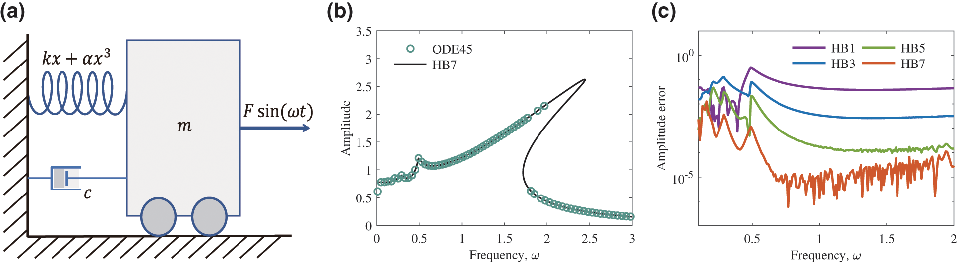
Figure 1: Illustration and computing results of the Duffing equation x¨+0.2x˙+x+x3=1.25sin⁡(ωt). (a) Illustration of a single degree freedom oscillator described by the Duffing Eq. (7). (b) Comparison of the amplitude-frequency response curves computed by HB7 and numerical integration method. (c) Errors of amplitude-frequency response curves bwtween the HB method and numerical integration method

It can be interpreted as a single degree of freedom oscillator with a cubic spring (Fig. 1a). In this paper, the parameters are set as c=0.2, k=1, α=1 and F=1.25. The amplitude-frequency responses were computed by using the HB and numerical integration methods. For simplicity, the n-th order HB method is denoted as HBn. It can be seen from Fig. 1b that the HB7 can obtain the entire hysteresis region, while ODE45 cannot. Outside the hysteresis region, the results of HB7 are almost the same as those of ODE45. Curves of error between the upper branches obtained by numerical integration and the HB methods are shown in Fig. 1c. The computing results of the HB become more accurate with the increase of N. Thus, the HB method is useful in studying the physics of frequency domain phenomena because parameter changes are more readily available with such semi-analytical methods [52]. Generally, several harmonics can obtain high-accuracy periodic solutions, which is especially attractive when the nonlinearity of the system is strong. Thus, the HB method has a wide range of applications, including but not limited to mechanical vibration [53], nonlinear circuits [6] and structural mechanics [52]. For example, Peng et al. [54] applied the HB method to investigate the performance of passive vibration isolators with cubic nonlinear damping. Zhu et al. [55] studied the application of the HB method on the active control of nonlinear vibration of viscoelastic orthotropic piezoelectric doubly-curved smart nanoshells with surface effects.

However, the HB method has a major drawback: the HB algebraic equation is difficult to derive. Eqs. (3)–(5) require a large amount of symbolic operations, especially when N is large [24,56–59]. Even with the help of computer algebra software the computational complexity brought by moderately large HB analysis (a dozen of harmonics) is still unaffordable. To overcome the derivation difficulties of the HB method, a series of new methods have been developed.

2.2 Incremental Harmonic Balance Method

The IHB method was proposed by Lau et al. [26] by combining the incremental procedure with the HB method. The principle is to add an incremental linearization process before using harmonic balancing. Besides, the IHB method is always guaranteed to converge [26], provided that appropriately small increments are chosen. Specifically, the IHB method performs Taylor series expansion of Eq. (1) at the non-singular solution x0

r(x,x˙,t)|x=x0+∂r∂xδx+∂r∂x˙δx˙=0,(8)

where δx=x−x0. Multiplying both left and right sides of Eq. (8) by hT, and taking the integral over a period T yields

Jδx^N=R,(9)

where

J=1T∫0ThT[∂r∂xh+∂r∂x˙hωD]dt,  R=−1T∫0ThTr(x,x˙,t)|x=x0dt.(10)

Eq. (9) is the IHB algebraic equation. Essentially, the IHB method can be regarded as a combination of the HB and Newton methods, but the sequence of the increment and the harmonic balance procedures is reversed [60].

The IHB method alleviates the derivation difficulty of the HB method, for the partial derivatives in Eq. (9) may decrease the degree of nonlinearity of the residual term. Thus, it has been widely used, especially in mechanical systems [9,61–63]. Lau et al. [64] analysed the periodic vibrations of systems with a general form of piecewise-linear stiffness characteristics by using the IHB method. However, the IHB’s alleviation in derivation costs are not significant. The residual vector and Jacobian matrix in the IHB method require analytical expressions, leading to extra complex symbolic operations. At the same time, the intermediate variables of the iterative process need to be repeatedly calculated. When using the IHB method to deal with nonlinear terms in non-polynomial form, the Galerkin integral needs to be computed using numerical integration methods, which is usually time-consuming [65]. References [61,66] pointed out that for discontinuous friction damping problems, the IHB method is not more efficient than numerical integration methods. Furthermore, since the IHB method discretizes the increments of the original equation, bifurcation solutions cannot be obtained [67]. Leung et al. [68] developed an IIHB method, which performs harmonic balance procedure on the original equation and linearizes the resulting algebraic equation for a Newton iteration process. The harmonic balance is on the original equation, bifurcated solutions into chaos can be handled [67]. In fact, the IIHB method exchanges the sequence of the increment and the harmonic balance procedures and is essentially a combination of the HB and Newton methods. Lu et al. [69] studied the nonlinear dynamics of latent mooring structures under vertical excitation using the IIHB method.

2.3 The IHB-DFT Method

To simplify the derivations, an intuitive way is to use time domain quantities at discrete collocations (sampling points) to replace the Fourier coefficients. That is combining frequency domain methods with DFT/IDFT technique. The IHB-DFT method, dating back to 1983 [27,70], is the crucial improvement to the IHB method. It can be divided into two categories according to the order of harmonic balance and increment procedures. The first algorithm (hereafter referred to as ALGO1) introduces the DFT technique to help compute J and R in Eq. (9) to avoid symbolic operations and minimize CPU time [71]. The second category (ALGO2) exchanges the order of increment and harmonic balance procedures [67]. Essentially, it is the DFT variant of the IIHB method. Consider the first-order Taylor series expansion of the HB algebraic Eq. (5)

∂r^N∂x^N|x^N=x^Nnδx^N+r^N|x^N=x^Nn=0,(11)

where the superscript n represents the number of iteration steps, δx^N=x^Nn+1−x^Nn. The corresponding Jacobian matrix is H=−∂r^N/∂x^N. Thus,

δx^N=H−1r^N.(12)

The DFT is used to obtain components of the residual vector r^N|x^N=x^Nn and Jacobian matrix H. One can equally divide the period into M points and define the collocation series: tk=kT/M, where k=0,1,…,M−1. Components of r^N can be calculated in the time domain by [72]

r^0=∑k=0M−1r(tk),    r^2n−1=∑k=0M−1r(tk)cos⁡(nωtk),r^2n=∑k=0M−1r(tk)sin⁡(nωtk),(13)

where n=1,2,…,N. The expressions of the Jacobian matrix H can be found in [73]. Similar to the IHB method, the last step is to update x^N by using Newton method following x^N+δx^N→x^N.

Reference [73] proved the equivalence of the ALGO2 and IHB methods. Considering that the ALGO1 and IHB are almost the same except for a DFT process, and even equivalent when a polynomial system is considered according to the sampling theorem [35] (details are given in Section 3.3). Therefore, we group these algorithms into a category called the IHB-DFT method. It is worth mentioning that the ALGO2 is usually referred to as the AFT-HB method in literature. However, we believe that it is not entirely consistent with the description by Cameron et al. (the originators of the name “AFT-HB”) themselves in their 1989 paper [28]. Details are introduced in Section 2.4.

From the IHB-DFT method, Cardona et al. [18] proposed a multi-harmonic method to analyse the nonlinear dynamic systems submitted to periodic loading conditions. The approach is based on the systematic use of the FFT. The exact linearization of the resulting equations in the frequency domain allows for obtaining a full quadratic convergence rate. Zhang et al. [74] used the IHB-DFT method to study the rigid rotor supported by ball bearings with the nonlinearity of Hertz contact and ball passage vibrations. Wang et al. [75] proposed a modified IHB (MIHB) method. The MIHB method uses the Broyden method for approximate Jacobian matrix, and its initial guess is given by the relevant linear algebraic equation. Ju et al. [65] proposed an efficient Galerkin averaging-incremental harmonic balance (EGA-IHB) method. It is based on FFT and tensor shrinkage. The integral is calculated by multiplying a constant tensor with a vector of Fourier coefficients, which reduces the calculation cost of the integral term and has better robustness.

2.4 Alternating Frequency-Time Harmonic Balance Method

Although the IHB-DFT method has dramatically simplified the derivations of algebraic equations, the incremental procedure still causes some symbolic operations. It reduces the generality of the method since additional derivation and coding are required for a new system. Therefore, some of the latest methods abandon the incremental process, such as the AFT-HB, TDC and HDHB methods introduced next. The main idea of the AFT-HB method was first proposed by Cameron et al. [28]. It is realized that the nonlinearities can be accurately evaluated in the time domain and transformed back into the frequency domain, to form a set of nonlinear equations which can be solved by NAEs solvers [76]. The AFT-HB method uses DFT/IDFT technique to convert the Fourier coefficients to and from the time domain quantities. That is

r^N=E∗r~M,(14)

where r~M=[r~0  r~1  …  r~M−1]T. r~k=r(tk), k=0,1,…,M−1 is the time domain quantity at collocation point tk. The transformation matrix E∗ corresponding to the DFT is

E∗=2M[1212⋯12cos⁡(ωt1)cos⁡(ωt2)⋯cos⁡(ωtM)sin⁡(ωt1)sin⁡(ωt2)⋯sin⁡(ωtM)cos⁡(2ωt1)cos⁡(2ωt2)⋯cos⁡(2ωtM)sin⁡(2ωt1)sin⁡(2ωt2)⋯sin⁡(2ωtM)⋮⋮⋱⋮cos⁡(Nωt1)cos⁡(Nωt2)⋯cos⁡(NωtM)sin⁡(Nωt1)sin⁡(Nωt2)⋯sin⁡(NωtM)].(15)

The superscript “*” on the right is only used to distinguish the forward and inverse of the Fourier transform. Correspondingly, the IDFT transformation matrix E is

E=[1cos⁡(ωt1)sin⁡(ωt1)⋯cos⁡(Nωt1)sin⁡(Nωt1)1cos⁡(ωt2)sin⁡(ωt2)⋯cos⁡(Nωt2)sin⁡(Nωt2)⋮⋮⋮⋱⋮⋮1cos⁡(ωtM)sin⁡(ωtM)⋯cos⁡(NωtM)sin⁡(NωtM)].(16)

Thus, Eq. (5) can be written as

E∗r~M(Ex^N,EωDx^N)=0,(17)

or

E∗r~M(x~M,EDE∗ωx~M)=0.(18)

Eq. (17) is the AFT-HB algebraic equation. It is necessary to keep time-frequency transform when solving Eq. (17), as shown in Fig. 2. The AFT-HB method converts the Fourier coefficients into time domain quantities, avoiding numerous symbolic operations and significantly improving efficiency. In addition, this conversion makes the nonlinear term r not have to be a polynomial function [74], which expands the applications. The AFT-HB method has been successfully applied in various physical systems, such as mechanical rotor systems [77–79], nonlinear oscillator systems [80,81], piezoelectric mechanical systems [82] and ground shaping systems [83], etc. For instance, Detroux et al. [84] applied the AFT-HB method for the computation of periodic solutions and their bifurcations in codimension-2 parameter space.

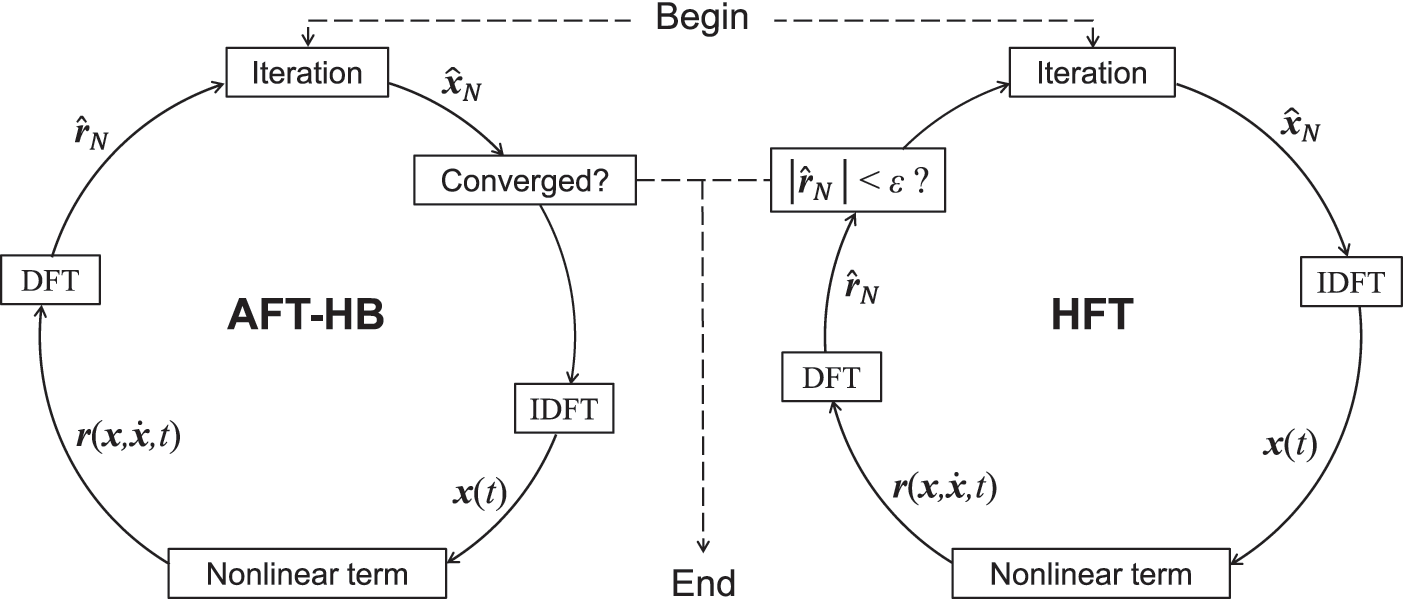
Figure 2: Direct iteration implementation of the AFT-HB method and the HFT method

Guillen et al. [85,86] proposed a hybrid frequency-time domain (HFT) method. As a variant of the AFT-HB method, the difference lies in the position where the two jump out of the iteration and the corresponding judgment conditions, as shown in Fig. 2. Poudou et al. [76,87] used the HFT method to analyse the dynamics of complex structures with dry friction dampers and noted that the method is directly applicable to more realistic structures found in the turbomachinery industry.

Fig. 3 shows the illustration of the HB, IHB, IHB-DFT and AFT-HB methods. The main difference between the IHB-DFT and the AFT-HB method is the incremental procedure, which causes that the AFT-HB algebraic equation is nonlinear however it is linear in the IHB-DFT method. In addition, the DFT technique is applied for the calculation of the Jacobian matrix in the IHB-DFT, while the replacement of nonlinear terms in the AFT-HB. As a result, under the condition of polynomial nonlinearities (details are given in Section 3.3), the IHB-DFT method is equivalent to the IHB method, while the AFT-HB method is proved as a time domain identity of the HB method. Considering the above differences, it is necessary to distinguish these two methods for accurate cognition.

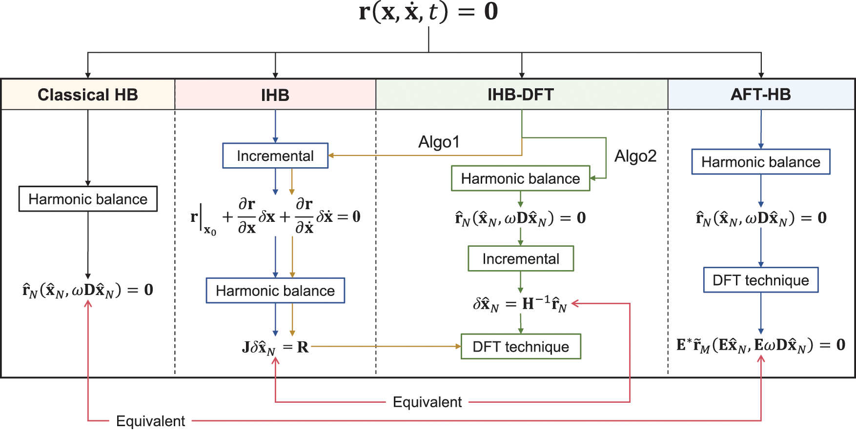
Figure 3: Comparison of the HB, IHB, IHB-DFT and AFT-HB methods

2.5 Time Domain Collocation Method

The derivation and calculation can be further simplified if the time-frequency domain transform is avoided. That is, all calculations are done in the time domain. The TDC method (also known as trigonometric collocation method [40]) is a representative method of this idea [29,30]. This method also uses Fourier base functions as trial functions. However, Dirac delta functions are used as test functions. Thus,

1T∫0Tδ(t−tk)rn(x^N,t)dt=0,  k=0,1,…,M−1.(19)

Dirac delta functions have the following properties:

δ(t−tk)={0,t≠tk∞,t=tk, ∫0Tδ(t−tk)dt={1,tk∈[0,T]0,tk∉[0,T].(20)

Eq. (19) can be written as

r~M(Ex^N,EωDx^N)=0.(21)

Eq. (21) is the TDC algebraic equation. It means the residual rn is a zero vector at collocations over a period. Residuals and unknowns in the TDC method are all time domain quantities without the need for time-frequency domain transformation. Thus, it is regarded as a full-time domain method. Since the trial functions are inconsistent with the test functions, the TDC method is generally not the Galerkin method. It is called the pseudo-spectral method in much literature to emphasize its difference from the Galerkin method [40]. The TDC method has been applied to the solution of many problems because of its intuitive, simple form and clear physical meaning. For example, Fornberg [88] investigated the problem of 2-DOF elastic seismic modelling. He found that the computing speed of the TDC method can reach hundreds of times that over of the finite difference method. Elschner et al. [89] solved the Symm integral equation; Dai et al. [34,36] analysed the Duffing equation and the binary airfoil model; Yue et al. [90] applied the TDC method to solve the periodic orbit of the relative motion of the spacecraft.

It is worth noting that Eq. (21) is a well-posed equation system with M=2N+1. When M>2N+1, it is overdetermined and is commonly satisfied in only a least-squares sense. Dai et al. [34] named the overdetermined version the ETDC method and gave the specific computing steps. The approximate solution x^N∗ for x^N makes r~M(Ex^N∗,EωDx^N∗)=R≠0, so that x^N∗ minimize the square error, RTR. The Einistein summation convention applies herein. To minimize RTR requires

∂∂x^N∗RTR=∂r~M∂x^N∗r~M=BTr~M=0.(22)

Eq. (22) is the ETDC algebraic equation. The dimension of the Jacobian matrix B of the collocation resulting system is M×(2N+1), and R is M×1. It is obvious that the ETDC algebraic equation is extended from the original TDC by multiplying BT on the left of r~M. For convenience, in this paper, the abbreviations “TDC” and “ETDC” will refer to M=2N+1 and M>2N+1 cases, respectively.

2.6 High Dimensional Harmonic Balance Method

The HDHB method was first proposed by Hall et al. [22], also known as the time spectral method [40]. Its principle is similar to that of the AFT-HB method, that is to replace the original HB algebraic system (5) with simple time domain quantities. The difference is that, in order to ensure the reversibility of DFT/IDFT x~M=Ex^N and x^N=E∗x~M, the HDHB method limits the number of collocation points M=2N+1, at this time E and E∗ are both square matrices and are mutually inverse matrices. After considering the above transformations, the HDHB algebraic equation can be written as

r~M(x~M,EDE∗ωx~M)=0.(23)

Eq. (23) is the HDHB algebraic equation. It has been proved that the TDC and HDHB methods are equivalent [29]. Therefore, the HDHB method is a pseudo-spectral method rather than a spectral method. It should be noted that the HDHB method is also equivalent to the AFT-HB method with M=2N+1. Besides, the nonlinear frequency domain (NLFD) method developed by McMullen and Jameson [91,92] is essentially identical to the HDHB method [33].

The HDHB method has been widely used, such as Duffing oscillator, Van der Pol oscillator, two-DOF airfoil, etc. [31,93,94]. Meanwhile, since the HDHB algebraic equation is well-posed, it is easier to solve implicitly. Thus, this method is most widely applied in the field of computational fluid dynamics (CFD) [95,96], such as the unsteady flow of turbine blades [97–101], aeroelasticity problems [102–104], etc. The HDHB method converts the unsteady periodic flow field solution into a steady flow field solution at discrete time points. Iterative computations can be accelerated using local time steps, multigrid methods, etc. At the same time, the implicit HDHB solver has also been developed [105–107], which further expands the applications. Several existing studies suggest that the efficiency of the HDHB solver can be further improved. For instance, Djeddi et al. [108] proposed a preprocessing technique that can improve the convergence of the harmonic balance solver, reducing the number of iterations by 50%–60% with the same accuracy. In conclusion, the HDHB method usually requires a relatively small number of harmonics to accurately simulate steady-state unsteady flow [44,109]. At the same time, solving transient oscillations is avoided, which dramatically saves the computational cost [95]. Compared with traditional methods, it has obvious advantages. At present, the HDHB method has been added to CFD software such as ANSYS CFX and SU2. Fig. 4 shows the CFD results of a pitching NACA0012 airfoil using the HDHB method, whose angle of attack as a function of time such that α(t)=αm+α0sin⁡(ωt). Governing equation is chosen as the Euler equation. The case has a free stream Mach number of 0.6, a mean incidence αm=2.89∘, α0=2.41∘, ω=0.097, and the pitching is about the quarter chord.

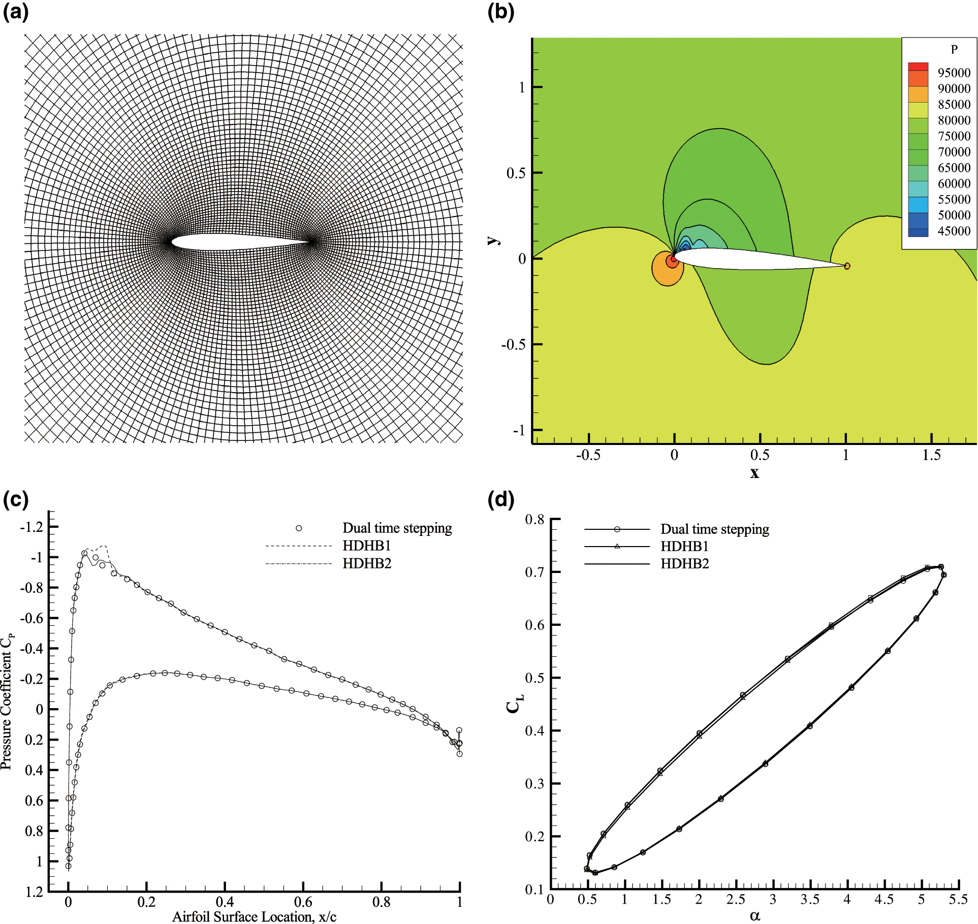
Figure 4: CFD results of a pitching NACA0012 airfoil using the HDHB method. (a) View of the block structured O-grid with 161 × 100 nodes. (b) HDHB2 unsteady pressure contours. (c) Surface pressure distributions with α=2.89∘. (d) Unsteady lift coefficient results

According to the existing literature results, the HDHB method presents instability when applied to CFD. Hall et al. [22] found that the non-convergence of the flow field appeared after increasing the number of harmonics and pointed out it is due to instability. Subsequent studies have been devoted to addressing the stability problem of the HDHB method. van der Weide et al. [110] studied the effect of excitation frequency and Fourier truncated order in the solver, giving the Courant-Friedrichs-Lewy (CFL) number constraint for the HDHB solver. Gentilli [111] found that a reasonable choice of the integration method or preconditioning can lead to a conditionally stable explicit format. Thomas et al. [96] pointed out that the stability is determined by the computing scheme of the source term, and systematically analysed various computing schemes and their corresponding stabilities.

3  Dealiasing Technique

Compared with other improvements to the HB method, it is obvious that the HDHB and TDC methods are the most convenient because they not only avoid the complex symbolic operations but also do not require continuous frequency-time domain transformations. However, neither the HDHB nor the TDC is equivalent to the HB because of the aliasing phenomenon, which leads to non-physical solutions. Besides, aliasing errors can cause influence on stability and convergence [112]. Many studies have been devoted to addressing this issue. They can be divided into two categories: numerical-filtering dealiasing and collocation-manipulating dealiasing. Recent studies have shown that the collocation-manipulating dealiasing methods can completely eliminate the aliasing of polynomial nonlinearities, and are therefore the more efficient approaches. In this section, dealiasing techniques have been fully discussed, including some recent advances and challenges that still exist.

3.1 Non-Physcial Solutions Caused by Aliasing Phenomenon

The concept of aliasing has been proposed as early as the last century. Intuitively, the cause of aliasing is the pollution of low-order harmonics by high-order harmonic components [31,36], as shown in Fig. 5. The time domain responses of high-order and low-order harmonics cannot be distinguished at the collocation points. Thus, the coefficients of discrete Fourier series are calculated inexactly.

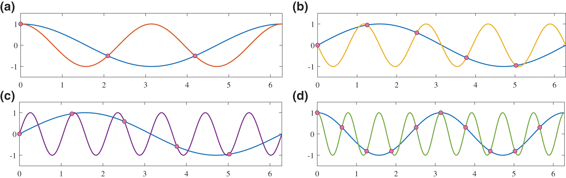
Figure 5: Illustration of aliasing. (a) cos⁡(2t)→cos⁡(t). (b) −sin⁡(4t)→sin⁡(t). (c) sin⁡(6t)→sin⁡(t). (d) cos⁡(8t)→cos⁡(2t)

Aliasing often leads to very serious non-physical solution problems [29,31,36]. We solved the Duffing Eq. (7) using the HDHB and the HB methods for comparison. Take N=2 as an example, the Fourier coefficients of nonlinear term x3 computing by HB2 are

f^HB=[34f^0f^1f^2f^3f^4]=[x03+34x12x3−34x22x3+32x1x2x4+32x0x12+32x0x22+32x0x32+32x0x423x02x1+3x0x1x3+3x0x2x4+34x13+34x1x22+32x1x32+32x1x423x02x2+34x12x2+34x23−3x0x2x3+32x2x32+3x0x1x4+32x2x4232x0x12−32x0x22+3x02x3+32x12x3+32x22x3+34x33+34x3x423x0x1x2+3x02x4+32x12x4+32x22x4+34x32x4+34x43].(24)

When using the HDHB2, the Fourier coefficients become

f^HDHB=[f^0+34(x32−x42)x1−32x2x3x4f^1+34(x12−x22)x3+32(x32−x42)x0+14x33−34x3x42−32x1x2x4f^2−34(x12−x22)x4−14x43+34x32x4−32x1x2x3−3x0x3x4f^3+14x13+34(x32−x42)x1−34x1x22+32x2x3x4+3x0x1x3−3x0x2x4f^4+14x23+34(x32−x42)x2−34x12x2−32x1x3x4−3x0x2x3−3x0x1x4].(25)

It reveals that the HDHB2 system contains all terms in the HB2 system, plus some additional terms, which cause non-physical solutions [31]. Fig. 6 gives the comparison of the amplitude-frequency response curves of the Duffing equation. The predictor-corrector method (PreCo, details are presented in Section 4.2) was used to compute the solution branch based on the open source tools NLvib 1.3 [113]. The initial solution point of continuation was selected as the HB solution at ω=0.01 (or ω=3.00 for backward continuation). Taking the HB curve as a benchmark, it can be seen that the HDHB results deviate from the benchmark. As shown in Figs. 6a and 6b, the HDHB method cannot compute the solution branch accurately, and it causes many non-physical solutions with N=1,2. When N=3, a large amount of non-physical solutions occurs around range ω∈(0.25,1).

Figure 6: Comparison of the amplitude-frequency response curves of the Duffing equation x¨+0.2x˙+x+x3=1.25sin⁡(ωt) computed by the HDHB and HB methods. (a) N=1. (b) N=2. (c) N=3

Next, we consider high-order cases. Fig. 7 gives the computing results with truncated order N as 4 to 9. We choose the frequency lies in the range [0.01,1.00] because the main difference between the results of the HDHB and HB are gathered here, as shown in Fig. 6c. As the truncated order increase, the results of the HDHB and HB become more consistent, which means that the continuation result of the high-order HDHB is reliable and increasing the number of harmonics can reduce the effect of aliasing, which is consistent with [31]. However, it is only true in some special cases. Through numerical experiments, we found that the HDHB continuation results are credible if and only when the initial solution point of continuation is in the lower frequency part. In fact, the HDHB algebraic equation remains a lot of non-physical solutions and not all of them can be obtained by continuation. Fig. 8a shows the Monte Carlo simulation of the HDHB and the RHB methods with N=3. That is, initial conditions are randomly generated for numerous computations to determine the probability of converging to any particular solution. It can be found that there is no non-physical solution of the HDHB method when the frequency ω<0.5. When the initial continuation point is selected with a larger frequency, the HDHB continuation procedure is often difficult to carry out. The initial estimates given often fail to converge to the correct solution branch. Besides, as N increases, the non-physical solution phenomenon of the HDHB method becomes more and more obvious, as shown in Fig. 8b. This makes the limitation of the HDHB’s initial continuation point selection more stringent. However, the HB method does not suffer from non-physical solutions, and the initial continuation point can be selected arbitrarily.

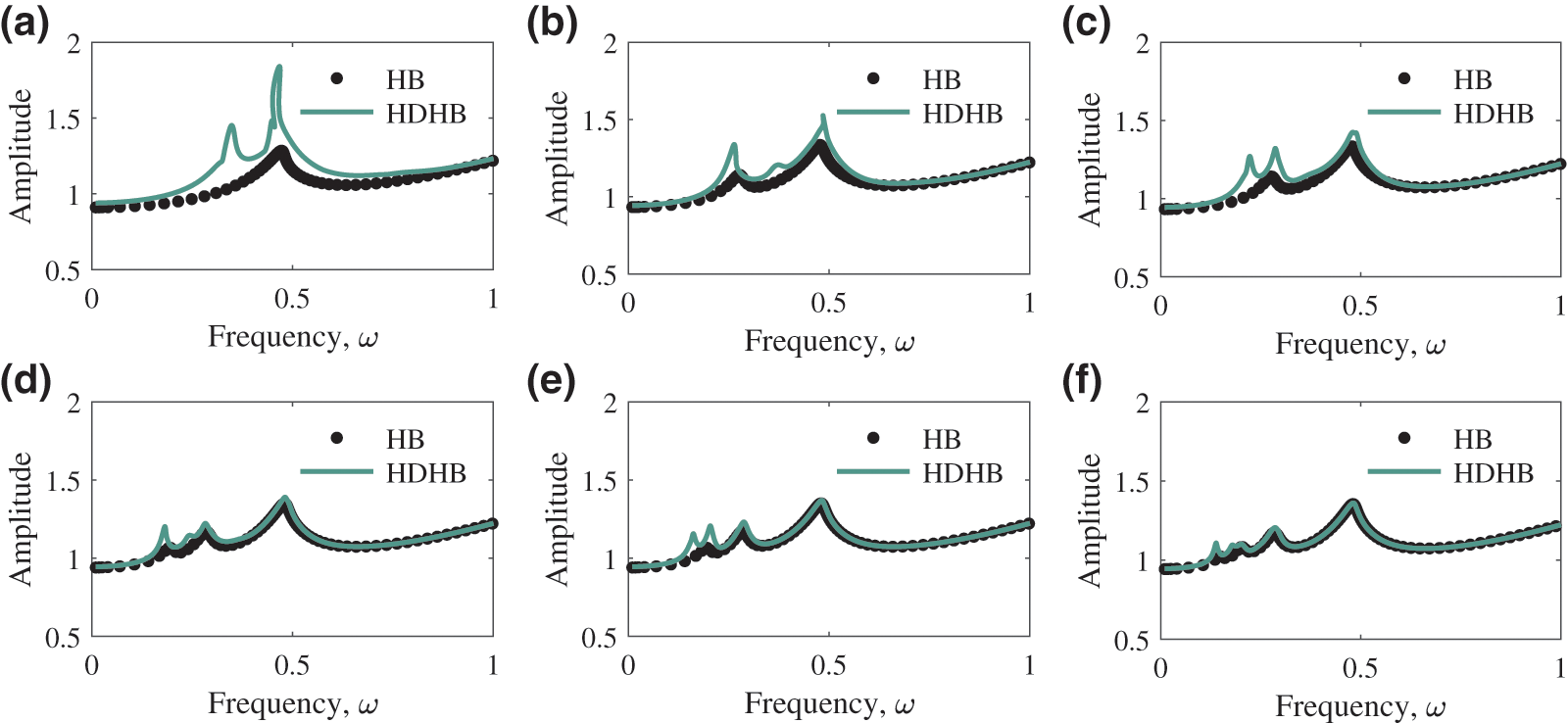
Figure 7: Amplitude-frequency response curves with high truncated orders. (a)–(f) N=4,5,…,9

Figure 8: Statistical distribution of solutions by the HDHB method based on the Monte Carlo simulation. (a) The number of non-physical solutions of HDHB3 in the frequency range [0.1,3]. (b) Variation of the number of non-physical solutions with the number of harmonics at ω=2.0

3.2 Numerical-Filtering Dealiasing Methods

A series of studies have been devoted to dealing with aliasing based on numerical-filtering, where the more effective ones are the truncated polluted harmonics (TPH) and the time spectral viscosity (TSV) methods [33]. The TPH method was first proposed by Orszag [114]. He developed a two-thirds rule and demonstrated that truncating all the polluted harmonics will remove aliasing terms for systems containing quadratic nonlinearities. That means zeroing the Fourier coefficients for all orders greater than a cut-off order nc. Specifically, the relationship between the cut-off order nc and truncated order N is given by nc≤2N/3. Orszag’s conclusion was generalized by LaBryer et al. [32] to all polynomial nonlinear systems, resulting in the so-called one-half rule. That is

ncN≤2ϕ+1,(26)

where ϕ is the highest degree of nonlinearity. The proposers did not assign a specific name to the relationship (26), and “one-half” was derived from the Duffing equation with ϕ=3. This paper uses the name “one-half rule” to refer to this relationship between nc, N and ϕ. This rule can be regarded as a Fourier coefficients filter that can be written as

x^Nf=G(ns)x^N,(27)

where G(ns) is commonly referred to as a low-pass Fourier filter or transfer function. ns is the scaled order, ns=πn/N introduced for convenience, n∈[0,N]. For the Duffing Eq. (7), it becomes

G(ns)={1,for  ns≤π/20,for  ns>π/2.(28)

Complete aliasing removal can be accomplished by filtering all orders that are polluted with non-physical terms. However, sharp cut-off functions may cause the algebraic system to be susceptible to the Gibbs-type phenomenon. Hou et al. [115] proposed a Fourier smoothing method to gradually damp out the highest frequency Fourier modes by choosing G(ns) to be

G(ns)=e−α(ns/π)m,(29)

where α and m are parameters that need to select properly. Fig. 9 shows the comparison of sharp cut-off and smoothing functions with α=36 and m=20. This scheme is a compromise between dealiasing and accuracy since the dealiasing occurs simultaneously with the filtering of coefficients of the true solutions. On this basis, LaBryer et al. [32] designed a temporal filter to improve computing efficiency. The TPH method performs well when used to solve Duffing equation. However, a serious problem is that it may not guarantee both the accuracy of the solution and the efficiency of dealiasing because of the lack of theoretical support.

Figure 9: Transfer function profiles for the frequency domain filtering schemes [32]

The idea of vanishing spectral viscosity concept was first proposed by Tadmor et al. [116–118] to damp the high-frequency content for retaining solution accuracy. McMullen et al. [92] used the TSV to coarser meshes in their multigrid cycle. Huang et al. [33] first suppressed the aliasing in the HDHB method by introducing the TSV, which improves the computational accuracy of the HDHB-CFD solver. That is to add a second-order TSV term to the Eq. (23) so that

r~M(x~M,EDE∗ωx~M)=ω2D2x~M,(30)

where the expression of ω2D2 can be found in [33]. The extent of the vanishing spectral viscosity in controled by the Fourier cut-off function ρn and it is taken to be

ρn={0,if  n≤p1,if  n>p,n∈[0,N].(31)

p is the cut-off number of harmonics. A first-order accuracy can be obtained with p=0 and spectral accuracy with p=N. The TSV method is similar to the TPH method for both of them filter the high-order coefficients in the HDHB solution [112].

The above methods can reduce the influence of aliasing errors and effectively suppress the non-physical solutions based on the idea of numerical-filtering. However, they reduce the computing accuracy because some meaningful parts of the true solution are filtered out, and its validity cannot be guaranteed when dealing with other systems. Meanwhile, the efficiency of these dealiasing techniques is only guaranteed at the numerical level with no theoretical support. Researchers were gradually turning to collocation-manipulating methods to obtain more reliable results.

3.3 Sampling Theorem and Oversampling

A natural thought is whether the aliasing phenomenon can be avoided by increasing the number of collocation points. Dai et al. [34] tried to eliminate the non-physical solutions by using the ETDC method. Statistical numerical simulation results illustrated that the probability of non-physical solutions decreases even to zero as more collocation points are chosen. However, the ETDC method uses the least square method to deal with the overdetermined equations caused by more than 2N+1 collocations, which is essentially a numerical dealiasing technique, and is no relevant theory to guide the choice of the collocation points. They used 20 collocation points to eliminate the non-physical solutions of Duffing equation introduced by the 2-order HDHB approximation, which is not general.

An ingenious attempt to overcome aliasing is the combination of the AFT-HB method and sampling theorem. Sampling theorem was first proposed by Shannon [35] and developed as one of the most important fundamental theorems in the field of signal processing. The theorem is described as follows:

Theorem 3.1 Sampling theorem. If the function f(t)=f(t+T) is a Fourier series with period T, i.e.,

f(t)=∑k=−Nk=Nf^(k)eikωt,(32)

with truncation order N, i=−1 is the imaginary unit. The DFT process

f^(n)=1M∑n=0M−1f(tk)e−in2πMk,  n=−N,…,N,(33)

gives exactly the Fourier coefficients for M≥2N+1.

According to the sampling theorem, when the sampling frequency is greater than twice the maximum frequency of the signal, the Fourier coefficients can be completely reconstructed without aliasing error. For Eq. (1) in this paper, if r is a polynomial function of x and x˙, it can be known from the convolution theorem that the maximum order of the Fourier series formed by r is ϕN. Thus, the number of collocation points M should satisfy M≥2ϕN+1 to keep the DFT process r^N=E∗r~M an identity. Combining the sampling theorem with HB-like methods yields some valuable properties. The IHB-DFT method is equivalent to the IHB method under the condition of polynomial nonlinearities, and the AFT-HB method is a frequency-time domain identity of the HB method. The latter provides an efficient way to dealiasing. Shown in Fig. 10 are the Monte Carlo simulation results of the Duffing Eq. (7) computed by AFT-HB2 and HDHB2 at ω=2.0. At this frequency, the Duffing equation has three physical solutions corresponding to the upper, lower and unstable branches, as shown in Fig. 1b. What can be seen is that the AFT-HB method eliminates non-physical solutions caused by the aliasing in the HDHB method.

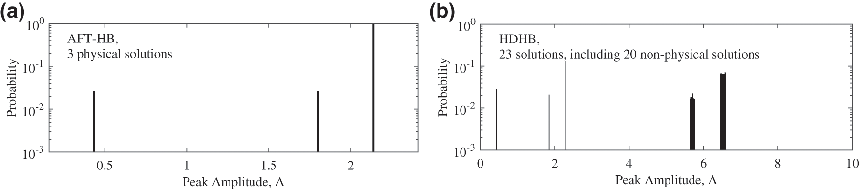
Figure 10: Monte Carlo simulation results of the Duffing equation computed by AFT-HB2 and HDHB2 at ω=2.0. (a) Results of the AFT-HB. (b) Results of the HDHB

However, the sampling theorem is oversampled. That is, the number of collocation points of the AFT-HB method is excessive. Table 1 shows the non-physical solutions computed by the AFT-HB method using the different number of collocation points. Lower number of collocation points can obtain only physical solutions, which means that M≥2ϕN+1 is unnecessary. Excessive collocation points will lead to the oversampling phenomenon that imposes an additional burden on the computation, especially when the polynomial power of r is high, or the truncated order N of the Fourier series is large. The practical application value of the AFT-HB method will be significantly reduced if hardware facilities are difficult to achieve such high-frequency sampling. It is possible that there is a value that serves as a cut-off for whether the solution behaves well or not (whether there is a possibility of non-physical solutions).

3.4 Rules of Aliasing

The key progress for dealiasing and anti-oversampling is the clarification of the rules of aliasing. The rules of aliasing of the pseudo-spectal method had been pointed out by Boyd [119]. Previous study demonstrated that the HDHB method is not a variant of the HB method, but a TDC method (pseudo-spectral method) in disguise [29]. Therefore, the aliasing phenomenon of the HDHB/TDC method can be explained with the help of the existing research on the rules of aliasing of the pseudo-spectral method. Thus, the principle beneath the aliasing phenomenon of the HDHB/TDC method can be illustrated as follows [36]:

Theorem 3.2 Rules of aliasing. If the interval α∈[0,2π] is discretized in time domain with uniform grid spacing h, then the wavenumbers (frequency domain value of the truncated order) in the truncated trigonometric series lies on the range n∈[−L,L], where L=π/h is the so-called “aliasing limit” wavenumber. Higher wavenumbers (|n|>L) will be aliased to lower wavenumbers na:

na=n−2mL,(34)

where na∈[−L,L], m is an integer.

The positive and negative of the wavenumbers correspond to the cosine and sine functions. The absolute value of wavenumber is the truncation order of the Fourier series.

Rules of aliasing are crucial in describing the relationship between the HB method and HDHB/TDC method. They are extracted from the analysis of the nonlinear term and therefore applicable to all the dynamical systems in general [36]. Most importantly, dealiasing research has had a basis of quantitative analysis instead of just staying at the level of numerical experiments. According to rules of aliasing, the corresponding aliasing condition between high-order and low-order harmonics can be clearly obtained. Specifically, for N=2 and M=2N+1=5. The spacing h is 2π/5 and the aliasing limit L is 2.5. The wavenumber that is greater than 2.5(2) will occur when the degree of nonlinearity ϕ≥2. Any wavenumber n beyond the range [−2.5,2.5] is aliased to na=n−5m, such that na∈[−2.5,2.5]. For example, wavenumber −4 (sin⁡(4t)) is aliased to 1 (cos⁡(t)), as shown in Fig. 5b.

3.5 Reconstruction Harmonic Balance Method

Based on the rules of aliasing, some recent studies have shown that the number of collocation points does not need to strictly follow the requirements of the sampling theorem. The HB method can also be reconstructed when fewer collocation points [37,73]. The sampling theorem makes the Fourier series formed by r not aliased, that is, harmonics in the range [−ϕN,ϕN] will not be aliased by high-order harmonics. However, the HB method only requires that the harmonics in the range [−N, N] are accurately determined. Therefore, it is an oversampling state when M≥2ϕN+1. The RHB method, based on equivalently reconstructing the HB method with pure collocations, has been developed to conquer the famous aliasing problem without losing computation accuracy. It was developed on the basis of a newly recovered dealiasing theorem illustrated as follows:

Theorem 3.3 Dealiasing. Suppose the nonlinear differential Eq. (1) is in polynomial-type nonlinearity with a degree of nonlinearity ϕ. Then, the aliasing phenomenon can be eliminated if the number of collocation nodes in the RHB method satisfies

M≥(ϕ+1)N+1.(35)

where N is the truncation order of the Fourier series.

To prevent high-order harmonics from being aliased in the range [−N, N], the number of collocation points M needs to satisfy M≥(ϕ+1)N+1. The method corresponding to this collocation strategy is the so-called RHB method. Its algebraic equation is consistent with the form of Eq. (17), that is

E∗r~M(Ex^N,EωDx^N)=0,(36)

where the only difference lies in the number of collocation points M. Fig. 11 shows the computing process of the RHB method. It can be seen that the RHB method also requires a continuously frequency-time domain transform, which is similar to the calculation flow of the AFT-HB method. However, based on the more advanced dealiasing theorem, the RHB method provides a new idea to decrease the limitation of the number of collocation points dramatically. Fig. 12 shows the illustration of aliasing in the frequency domain of the HDHB, RHB and AFT-HB methods. For the HDHB method, the higher wavenumber is aliased to a lower wavenumber in the range [−N, N], which is the computed range of the HB method. For the RHB method, the aliased lower wavenumber is “pushed” out [−N, N] thanks to more collocation points. Although the higher wavenumber in [N,ϕN] cannot be distinguished from wavenumbers lies in [−ϕN,N], the calculation will not be affected because of the precise calculation of Fourier coefficients in [−N, N]. However, the AFT-HB method takes more collocations so that oversampling phenomenon occurs.

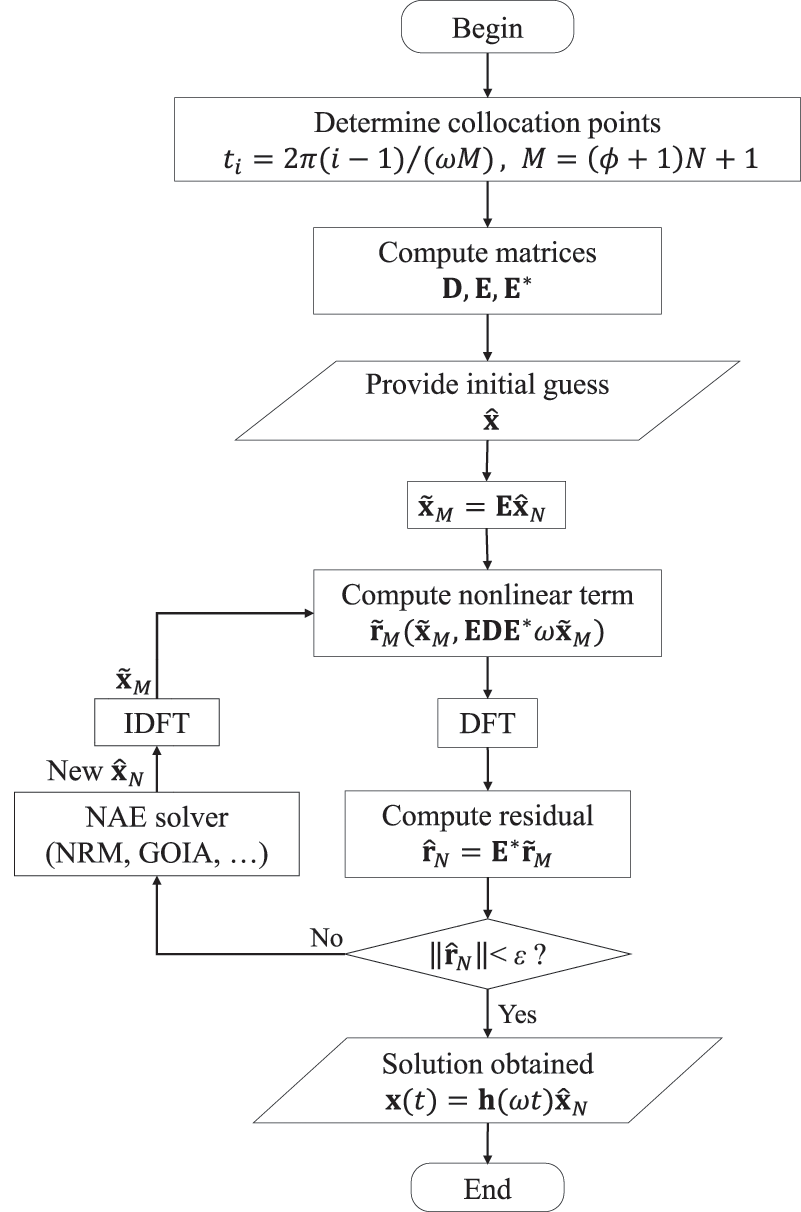
Figure 11: Computing flow of the RHB method

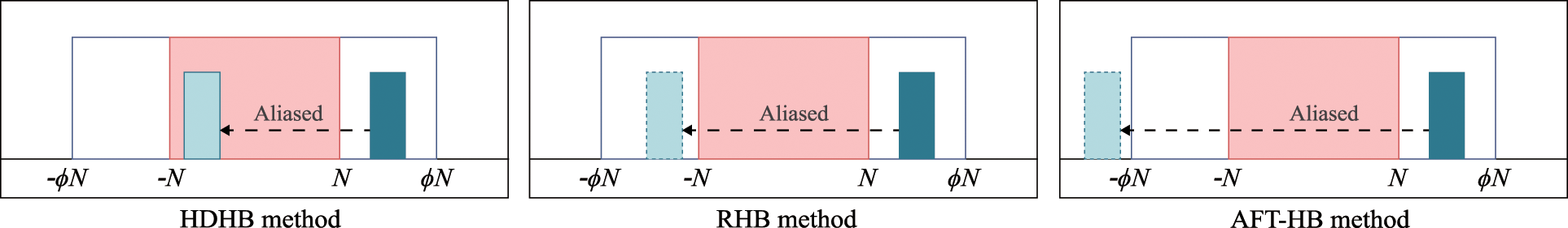
Figure 12: Illustration of aliasing and dealiasing of the HDHB, RHB and AFT-HB methods in frequency domain

There is an important equivalent identity r^N≡E∗r~M holds when M satisfies Eq. (35) [37], as described below:

Theorem 3.4 Conditional equivalence. If number of collocation points M, truncated order of harmonics N and degree of nonlinearity ϕ satisfy M>(ϕ+1)N, then the RHB method and the HB method are equivalent.

Dai et al. [37] found that the degree of aliasing is determined by an “aliasing matrix”. As the number of collocation points increases, the non-zero elements in the aliasing matrix gradually decrease. When the number of collocation points satisfies the Eq. (35), the aliasing matrix is an all-zero matrix. Shown in Fig. 13a is the aliasing matrices with N=3 and ϕ=3. The number of collocation points was selected as 7, 9, 11 and 13, respectively. The non-zero elements were marked as orange, implying that the harmonics correlated by these elements were mixed. It can be seen that the non-zero elements gradually decrease with the addition of collocation nodes. The corresponding amplitude-frequency response curves are given in the Figs. 13b–13e. It shows that computing errors occur if the number of collocation points is insufficient. Once M=(ϕ+1)N+1, the RHB method produces almost the same result as the HB method. Solutions are confined to the physical ones once the minimum collocations are satisfied, otherwise, non-physical solutions may occur [37]. Meanwhile, the RHB method dramatically improves computational efficiency because it reduces the number of collocation points required by the sampling theorem. Fig. 14 shows the computing time of the AFT-HB method and its ratio to the RHB method when dealing with cubic and quintic Duffing equations. It can be seen that the RHB method could be more than 2–3 times faster once high-order harmonics are involved.

Figure 13: Variation of the aliasing matrix and its impact on computing results. (a) Illustration of the aliasing matrix changing with the number of collocation points M from 2N+1 to (ϕ+1)N+1. The difference in the number of collocation points between each matrix is 2 (b)–(e). Amplitude-frequency curves corresponding to the above aliasing matrices computed by the HB and RHB methods

Figure 14: Computing time of the AFT-HB and RHB methods and the ratio between them when dealing with cubic and quintic Duffing equations. (a) Cubic nonlinearity. (b) Quintic nonlinearity

When r is in non-polynomial form, even a finite term of x makes r a Fourier series with infinite non-zero terms. Fortunately, we can use the recast technique [51,120] to deal with rational fractional and basic transcendental functions type nonlinear systems. However, there is a lack of relevant theory for dealiasing general nonlinear systems especially non-smooth cases. Currently, the sampling rate is usually given by experience or trial calculations [40]. According to the FFT theory, it is generally taken as a positive integer power of 2, to pursue 𝒪(Mlog⁡M) operations [121].

3.6 Classifications of the HB-Like Methods

There are several approaches to classify the existing HB-like methods. Krack et al. [40] classified some HB-like methods in their monograph. The classification standard resides in whether the unknowns and/or the residual are formulated in time or frequency domain, as shown in Fig. 15. It is worth noting that since the summary by [40] is not comprehensive, appropriate supplements were made in this paper. It should be emphasized that the IHB-DFT, ETDC, AFT-HB and RHB methods appear in two different blocks since the time domain unknowns are used to compute the nonlinearities in the ETDC and AFT-HB/RHB, and Jacobians in the IHB-DFT. That is, unknowns are continuously transformed in frequency and time domain. From this point of view, the HB-like methods can be divided into three types: frequency domain methods (HB, IHB), semi-time domain methods (IHB-DFT, AFT-HB, ETDC) and full-time domain methods (HDHB, TDC).

Figure 15: The HB-like methods distinguished by the formulated domain of the unknowns and residual

In addition, the classification approach according to the type of test function is also an alternative. Considering that all the existing HB-like methods are weighted residual approaches and Fourier series are selected as trial functions. Substituting this approximation into the differential equation generally leads to a residual term. There are two main ideas to deal with residual terms according to existing methods. i) Spectral type, test functions are selected the same as trial functions, which leads to a Galerkin method. The HB, IHB and IHB-DFT methods fall into this category, as does the RHB method due to its equivalence with the HB method. ii) Pseudo-spectral type, Dirac delta functions are used as test functions, which means residual to be zero at discrete time domain collocations. Pseudo-spectral type is composed of the HDHB, TDC and ETDC methods. One of the difficult issues facing this classification is the attribution of the AFT-HB method with the number of collocation points M≤(ϕ+1)N. Noticing the existence of the aliasing phenomenon, there is

E∗r~M=r^N′≠r^N,(37)

where r^N′ is the aliased Fourier coefficients of the nonlinear term r. It is known that the aliased high-order harmonic coefficients are mixed into the low-order harmonic coefficients, so the test function can be regarded as a simple sum of high-order and low-order trigonometric functions. Take the AFT-HB2 with M=7 and x3 as an example. When the aliasing limit L=3.5, higher wavenumbers ±4, ±5 and ±6 are aliased to lower wavenumbers ∓3, ∓2 and ∓1. For instance, the Fourier coefficient in r^N, with wavenumber equals 1 is

1T∫0T[cos⁡(ωt)+sin⁡(6ωt)]⋅rn(hx^N,hωDx^N,t)dt=0,(38)

where cos⁡(ωt)+sin⁡(6ωt) is its test function. Thus, the AFT-HB method with the number of collocation points M≤(ϕ+1)N can also be regarded as a spectral type method.

Some HB-like methods can be unified based on different collocation points [37]. A schematic diagram of the collocation-based harmonic balance framework is presented in Fig. 16. When the number of collocation points M is in the range of [0,2N+1), there is no corresponding HB-like method. Since the harmonic balance algebraic equation corresponding to this range is underdetermined, the number of collocation points is no sense. M=2N+1 corresponds to the HDHB/TDC method. There are two forms when increasing the number of collocation points, one is to keep the residuals as the time domain quantities (ETDC), and the other is to transform the time domain residuals to the frequency domain using the DFT technique (AFT-HB). It should be noted that the algebraic Eqs. (17) and (23) are equivalent when M=2N+1. M=(ϕ+1)N+1 corresponds to the RHB method. When M≥(ϕ+1)N+1, the RHB/AFT-HB methods are equivalent to the HB method. From the collocation-based harmonic balance framework, the HB-like methods except the HB method can be divided into two categories: incremental-based and collocation-based. The IHB and IHB-DFT methods can be regarded as incremental-based methods, and collocation-based methods for the AFT-HB, HDHB/TDC and ETDC methods.

Figure 16: Illustration of the collocation-based harmonic balance framework that unifies the HB, the AFT-HB, the RHB, the HDHB/TDC and the ETDC methods

4  Solving the Harmonic Balance Algebraic Equations

The harmonic balance procedure is not the final step before obtaining the periodic solution of the nonlinear system. Essentially, the HB-like methods transform the original differential system (or differential-algebraic system) into an algebraic system, which may have complex dynamics, such as multiple or even infinity steady-state solutions [122,123]. Therefore, accurate and efficient methods for solving harmonic balance algebraic equations are worth studying. In this section, different algebraic solution strategies suited for solving harmonic balance algebraic systems have been reviewed. In some cases, it is necessary to obtain the full response of the system with a certain parameter, which includes a series of solution points. Therefore, we then focus on the continuation techniques. Finally, we have discussed the existing convergence and stability theories to provide the necessary theoretical support for the whole process of applying the HB-like methods.

4.1 Algebraic Equation Solution Strategies

The most commonly used methods for solving harmonic balance algebraic equations are the Newton-Raphson method (NRM) and quasi-Newton methods [40]. The principle of the Newton method is to expand residual of an algebraic system in a Taylor series around the current estimate state xk, where k means the number of the current iteration step. Then, the next estimate xk+1 is determined using xk and the Jacobian matrix corresponding to the partial derivatives of nonlinear functions to states. It has a simple form and converges very quickly. However, it is sensitive to the initial guess and cannot guarantee the accuracy of the solution if an approximately singular or ill-conditioned Jacobian is encountered [52]. Quasi-Newton methods extend the idea of the secant method in the one-dimensional case to equation systems, such as Broyden method [124]. Ling et al. [71] pointed out that it has better stability than NRM. The Broyden algorithm needs more iterations to converge, but since there are fewer operations involved at each iteration, it turns out to be faster than the NRM. Moreover, the convergence of the method is nearly always guaranteed, even with a poor initial guess [85]. It has been successfully applied in the solution of harmonic balance algebraic systems [75].

Homotopy methods offer an alternative to computing all solutions of harmonic balance algebraic systems. They are divided into two types: Linear homotopy [125] and polyhedral homotopy [126]. In addition, Groebner basis [123], rational univariate representation [127] and multiplication matrix [128] methods are also alternative. There is a series of scalar homotopy methods based on the Newton scalar homotopy function [129–133]. The scalar homotopy methods do not require the inversion of the Jacobian matrix. They far outperform the NRM when the Jacobians are almost singular or severely ill-conditioned. At the same time, the scalar homotopy methods are insensitive to initial guesses and can handle overdetermined and underdetermined algebraic equations [52]. Therefore, these methods are also effective methods for solving harmonic balance algebraic equations, such as the global optimal iterative algorithm (GOIA) solver. Shown in Fig. 17 is the convergence history curves for the NRM and GOIA solvers with different frequencies when solving Duffing equation using the RHB method. The initial guess of the unknown Fourier coefficients was selected as zero, so that it gets farther from the real solution as the frequency increases. When the frequency is less than 0.4, the NRM can obtain residuals of the order of 10−16 in only a few iterations (about 10), while the GOIA requires hundreds of iterations. However, when the frequency is greater than 0.5, the NRM falls to a stagnant point. The GOIA becomes a better choice for its robustness. Therefore, trial calculations can be performed in advance to select a NAE solver. This usually does not incur a large computational cost.

Figure 17: Convergence history for the NRM and GOIA solvers with different frequencies when solving Duffing equation. (a)–(f). ω=0.2,0.3,…,0.7

There are also two other approaches. One is to solve the harmonic balance algebraic equation by pseudotime method [134]. That is to add a pseudotime derivative term so that the algebraic equation becomes a differential equation, which can then be solved by the numerical integration methods [135–137]. Attar [138] proved that the pseudotime method is equivalent to the Fourier enveloping method [139,140] when solving a class of periodic problems. The pseudotime method has obvious advantages when calculating large nonlinear problems, such as CFD [22,44,100,108,109], because there is no need to calculate the Jacobian matrix. However, it is extremely sensitive to initial guesses and converges much slower than NRM, with high integration costs. Therefore, this method is not recommended unless the Jacobian matrix is not available or involved [52]. Another way is to handle harmonic balance algebraic equations by optimization procedures. In other words, regarding the solution of the harmonic balance algebraic equation as an optimization problem. For instance, Thothadri et al. [141] combined the harmonic balance principle and bifurcation theory techniques to form a constrained optimization. Ahmadian et al. [142] used unconstrained optimization to identify the IHB algebraic equation for modelling bolted lap joints. Liao et al. [143] derived a constrained maximization problem based on the HB method and the Hill method to predict the maximum amplitude. Liu et al. [144,145] proposed a time-domain minimum residual method with energy balance.

In addition to the influence of different methods, there are some methods to improve the accuracy and convergence of the harmonic balance algebraic equation. For example, the sparseness of nonlinear terms can be used to reduce the dimension of algebraic equations, reducing the workload of solving and the impact of rounding errors [146,147]. Normalizing the system through preprocessing can improve the convergence when the magnitude of the variables is large, or the dimensions are different [37,40].

4.2 Continuation of Solution Branches

When studying nonlinear responses, we are often interested in the parameter response of the system, that is, the set of solutions corresponding to the free parameters (such as frequency). The easiest way is the sequential continuation method, also known as parameter sweeping. This method selects a series of parameters according to the magnitude, calculates the solution corresponding to the first parameter, and then uses the solution as initial guess to calculate results of the next parameter, and so on. It is simple to implement because the whole calculation process only needs to select the initial value 1 or 2 times. However, at jump points, the algebraic equations may not converge due to the distance from the previous step to the true solution. In addition, the solution branch between two jump points, such as the unstable solution branch of Duffing equation, cannot usually be solved directly. It is necessary to re-select the initial point on the solution branch for continuation, and there is no guarantee that the subsequent results are still in the expected solution branch. Therefore, the sequential continuation method is not reliable. In some cases, it can only be used for trial calculation of the system.

One commonly used continuation technique is the PreCo method [40]. The main idea of the PreCo method is to start from the current solution point and perform one-step estimation and prediction forward (often along the gradient direction). Iterate over the predicted points until their distance from the true solution satisfies the error limit. Use the corrected solution point as the initial solution point for the next calculation. This process is repeated until the entire solution branch is computed [40,148]. The PreCo method is often used in combination with the AFT-HB method [40,82,149]. Another commonly used method is the asymptotic numerical method (ANM) [150,151]. The ANM expands the solution branch into a high-order Taylor series with respect to the arc length parameter, which can be viewed as an alternative to the prediction step. Correction steps can be avoided by taking the step size to be within the convergence range that satisfies the Taylor expansion [51,152]. The main difficulty of the ANM is how to efficiently calculate the coefficients of high-order Taylor series. To solve this problem, the algebraic system is usually reconstructed into a form containing only quadratic nonlinear terms using auxiliary variables and augmented equations [149]. Compared with the PreCo method, the ANM is more robust [153]. However, the ANM is only suitable for sufficiently smooth nonlinear systems. When dealing with non-smooth mechanical systems, regularization methods are usually required to approximate smooth systems [40]. Woiwode et al. [149] carefully compared the PreCo method and the ANM with some concrete examples, and gave the recommended applications of the two methods. Reference [154] summarized the use of control methods to compute geometrically nonlinear equilibrium paths.

The above solution branch continuation method has been widely used in the solution of harmonic balance algebraic equations [155]. For example, Cheung et al. [156] proposed an incremental arc-length method combined with a cubic extrapolation technique to track the response curve, reducing the number of iterations required for convergence. von Groll et al. [157] developed a numerical method for the dynamics of rotor/stator interactions. The method determines the stability of the solution while calculating the periodic solution, marks the turning and bifurcation points, and uses the continuation method to track the solution branches. Cochelin et al. [51] proposed the recast technique to preprocess the system into quadratic polynomial form before applying the HB method and then used the ANM to solve it. The recast technique can be applied to a large class of nonlinear systems, reducing the difficulty of deriving harmonic balance equations from these systems. In addition, Louis et al. [158], based on their research, developed MANLAB, a Matlab software package for interactive continuation and bifurcation analysis of nonlinear systems of equations. Combining the ANM with the dual fundamental frequency HB method, Guillot et al. [159] achieved a continuation of the quasi-periodic solution branch, where the two fundamental frequencies can be unknown and may vary along the solution branch. Later, Guillot et al. [160] applied the method to the continuation of the periodic orbits of delay differential equations. A smooth bifurcation tracking algorithm with mutual parameter dependencies was developed by Mélot et al. [161]. This method is based on the HB method, combined with the arc-length method and the boundary technique, to form a minimum extension system. It can effectively determine the stable region of the system, which provides feasibility for the optimization of tooth profile modification of large gear transmissions.

4.3 Non-Smooth Systems

It is worth mentioning that some studies focus on the application of the HB method in solving non-smooth systems, which widely exist in mechanical engineering and electrical engineering disciplines, etc. [162–164]. Non-smooth nonlinear terms in the equations can cause jump discontinuities of the solution. That leads to the inapplicability of most of the integration methods and the HB-like methods are way out of this phenomenon [40]. The AFT-HB method is one of the most widely used techniques for solving non-smooth systems [165]. Nevertheless, considering the systems that can comprise distinct states so that the nonlinear functions are only piecewise defined, the AFT-HB method inherently induces inaccurate derivatives [164]. The combination of the ANM and HB-like methods may be an efficient way to deal with non-smooth due to its computationally robust and efficient continuation of the solution. However, for general nonlinearities, the quadratic recast is difficult, and the artificially smooth procedure required by the ANM leads to inaccuracies compared to the non-smooth model [40]. Up to now, the application of HB-like methods in general non-smooth dynamical systems still needs further research. There are many studies devoted to applying various HB-like methods to various specific problems.

Kim et al. [166] introduced generalizations of the classical HB method that result in superior convergence rates and superior modes of convergence by one or more expansion functions that possess the same degree of continuity as the exact solution. Petrov et al. [167] proposed an analytical formulation of the HB method for piecewise linear friction interface elements for the analysis of structural dynamical problems in the frequency domain. But this approach is only applicable to special types [164]. Krack et al. [164] extended this method to generic systems with an arbitrary number of distinct states, such as structural dynamical systems with conservative and dissipative nonlinearities in externally excited and autonomous configurations. This method allows for an analytical formulation of the high-order harmonic balance method for the dynamic analysis of systems with distinct states and is superior to the AFT-HB method in terms of accuracy and computational efficiency. Miguel et al. [168] proposed a new method for approximating both the Bouc-Wen and LuGre hysteresis loops analytically through a truncated Taylor series as a simple and effective smoothing procedure to enable the use of the HB method. Pei et al. [169] applied the IHB and AFT-HB methods to the analysis of the dynamics of the piecewise linear oscillator and confirmed the robustness of the HB-like methods. Chen et al. [170] presented a study on the non-smooth system of a floating network structure using the IHB method, especially the periodic solutions of bifurcation analysis.

4.4 Convergence Theories

Convergence is important for determining the scope of application of the HB-like methods. The convergence theories of the Fourier series were systematically given by Dirichlet and Riemann 200 years ago. However, they do not converge at the same rate as the Fourier truncation [171]. The research on the convergence of HB-like methods can be traced back to 1965. Urabe [58] proposed the existence and convergence theorems of approximate periodic solutions of the HB method for non-autonomous nonlinear systems. He studied ordinary differential systems in the form of r(x,x˙,t)=x˙−v(x,t)=0, and assumed that v(x,t) and its first derivative with respect to x are continuously derivable, that is, v(x,t) is of class 𝒞1 functions [40]. At the same time, he restricted the periodic solution to being isolated. Under the above constraints, he proved that when the order of the HB method N→∞, the HB approximation converges to the exact solution uniformly and gave the error limit. Urabe also proved that if an approximate periodic solution is obtained, there is a real periodic solution near the approximation. The above conclusion was later extended to an autonomous system by Stokes [172]. However, Urabe did not give the rate of convergence.

In 1986, Tadmor [173] proved that if the true solution x(t) is an analytic function (a function given locally by a convergent power series, which is a subset of 𝒞∞ class functions), and the truncation order is greater than a certain positive integer N0, the error between x(t) and its harmonic balance approximation xn(t,⋅) grows with the truncation order is exponentially convergent, i.e.,

‖xn(t,⋅)−x(t)‖∞<Ye−cN,  N>N0,(39)

where Y>0, c>0. The values of Y, c and N0 are determined by the actual model. This shows that increasing the order can improve the accuracy of the HB analysis. Fig. 18 shows the results of the RHB convergence study of Duffing equations x¨+0.2x˙+x+x3=1.25sin⁡(ωt) and x¨+0.2x˙+x+x5=1.25sin⁡(ωt) at ω=0.2. The result of HB200 is chosen as the benchmark. It is seen that the convergence rate of the RHB method is exponential. Due to equivalence with the HB method, the RHB method also follows the Eq. (39).

Figure 18: Computing error varying with the adopted order for the RHB method. (a) ϕ=3. (b) ϕ=5

However, the lack of a pre-asymptotic convergence theorem reduces the practical significance of the aforementioned research since the search for N0 still needs to rely on numerical experiments or experience. In fact, researchers often use the results of numerical integration to calculate the accuracy of harmonic balance analysis to judge whether the selected harmonic truncation order is appropriate, which is very unfavourable for the practical application of HB-like methods. Furthermore, no strict convergence theorem is available for systems of differential-algebraic or ordinary differential equations, especially when there are discontinuous terms in the equations. In 2019, Krack et al. [40] used numerical methods to point out that the HB method has a polynomial convergence rate when applied to non-smooth systems. Starting from the smoothness and continuity of the nonlinear term, Wang et al. [171] systematically analysed and deduced the convergence rate of the HB method, and established the harmonic balance error estimation theory for nonlinear systems with various smoothness. In addition, they found that when the nonlinear term is discontinuous or has some special low smoothness, the convergence speed of the HB method is different from that of the Fourier truncation, and the former is usually slower than the latter. Currently, the research by Wang et al. is the most complete and comprehensive work on the convergence of the HB method, which provides theoretical support for the further development and practical application of the HB-like methods.

4.5 Stability Analysis

In all cases, even though the HB-like methods can find a solution, they do not account for the stability of solution [174]. The stability of the solution can be determined using the Lyapunov-Floquet transform [66,175–178]. When the transformation matrix has an eigenvalue whose modulus exceeds 1, instability occurs; when the eigenvalue is less than −1, there is a period-doubling bifurcation. At the same time, the Floquet theory also gives the monodromy matrix from which the nature of bifurcation is known [179]. However, this method is needed to work in the time domain to obtain the monodromy matrix. The frequency method (Hill’s method) can be used to determine stability to avoid additional time domain processing [174]. Perturbation is set to truncated Fourier form, which is similar to von Neumann stability analysis [180]. Then, the equations are linearized and stability is judged from the eigenvalues of the coefficient matrix. This method is described in the references [174,181,182]. Hill’s method has two major drawbacks, i) redundant eigenvalues can lead to qualitatively wrong results; ii) the problem dimension scales with the truncation order. There is no conclusion as to which method is more suitable for the periodic solution computed by the HB-like methods.

5  Conclusions

Various HB-like methods were reviewed in this paper. First, the principles of these methods were discussed. The HB-like methods were categorized into frequency domain and time domain methods. Time domain methods were subdivided into semi-time and full-time domain methods. It is worth emphasizing that an IHB-DFT method has been defined to correct the previous misunderstandings of the AFT-HB method.

Next, the advantages and disadvantages of the HB-like methods were summarized. Table 2 gives the performances of the representative HB-like methods. The collocation-based methods are the most concise for derivation difficulty, which is evaluated by the number of symbolic operations. The derivation of the IHB-DFT method is more difficult than the collocation-based methods due to the introduction of the incremental process. For the difficulty of algebraic equation solving, the IHB and IHB-DFT methods perform the best since they have linear algebraic equations due to the incremental process. The HB algebraic system is hard to solve because of the existence of complex symbolic expressions, especially in high-order cases. The generality of the HB and IHB methods is the worst because of their re-derivations for new systems. As the DFT technique avoids the frequency domain calculation of nonlinear Fourier coefficients, the IHB-DFT performs better than the IHB method. The most general methods are the collocation-based methods. Their algebraic form does not change with the problem under consideration. In terms of accuracy, the IHB-DFT, AFT-HB, and RHB methods are the same provided that the rounding errors are ignored since they are equivalent to the HB (or IHB) method. Specifically, rounding errors can cause slight differences, e.g., the RHB’s accuracy is slightly higher than that of the AFT-HB method [37]. Affected by aliasing, the accuracy of the HDHB/TDC and ETDC methods is lower. In general, the time domain methods have obvious advantages over the frequency domain methods.

The dealiasing technique was also explored. Aliasing is one of the main challenges encountered by the time domain methods because the non-physical solution phenomenon arising from aliasing seriously affects the calculation accuracy. The RHB provides an efficient way to eliminate the non-physical phenomenon pertaining to time domain methods, and it is essentially an optimal reconstruction of the HB method via equivalently replacing the harmonic balancing with simple time domain collocations. The aliasing matrix gives a collocation-based framework to successfully incorporate the HB, the AFT-HB, and the HDHB methods into a unity. Another taxonomy for the HB-like methods has been developed based on this framework. In addition to the HB method, the existing HB-like methods can be divided into incremental-based methods and collocation-based methods. This system of classification helps to distinguish the semi-time domain methods IHB-DFT and AFT-HB. Finally, the methods for analysing harmonic balance algebraic equations were briefly introduced.

Based on the detailed review, three future directions are suggested:

  i)   Aliasing is unavoidable in the case of non-polynomial nonlinearities [73]. Although the recast technique can be used to deal with rational fractional and basic transcendental functions type nonlinear systems [51], there is a lack of relevant theory for dealiasing general nonlinear systems, especially non-smooth cases.

 ii)   Attributed to the ill-conditionedness of the resultant nonlinear algebraic equations, the accuracy of the existing methods shows a decreasing effect, especially when extremely high-order harmonics are included. Therefore, advanced precondition techniques will be required to improve the present HB-like methods.

iii)   Once the periodic response of the nonlinear system consists of incommensurable frequencies, the single-frequency methods have to include a number of harmonics (hundreds) to approach the real response, which severely restricts the efficiency of the algorithm. Methods for multiple fundamental frequencies may be effective approaches to deal with this problem.

Funding Statement: This work was supported by National Key Research and Development Program of China (No. 2021YFA0717100) and National Natural Science Foundation of China (Nos. 12072270, U2013206).

Conflicts of Interest: The authors declare that they have no conflicts of interest to report regarding the present study.

References

1. Kapania, R. K., Yang, T. (1987). Buckling, postbuckling, and nonlinear vibrations of imperfect plates. AIAA Journal, 25(10), 1338–1346. https://doi.org/10.2514/3.9788 [Google Scholar] [CrossRef]

2. Li, S., Yuan, J., Lipson, H. (2011). Ambient wind energy harvesting using cross-flow fluttering. Journal of Applied Physics, 109(2), 026104. https://doi.org/10.1063/1.3525045 [Google Scholar] [CrossRef]

3. Molnár, T. G., Dombóvári, Z., Insperger, T., Stépán, G. (2018). Bifurcation analysis of nonlinear time-periodic time-delay systems via semidiscretization. International Journal for Numerical Methods in Engineering, 115(1), 57–74. https://doi.org/10.1002/nme.5795 [Google Scholar] [CrossRef]

4. Liao, H. (2018). The reduced space method for calculating the periodic solution of nonlinear systems. Computer Modeling in Engineering & Sciences, 115(2), 233–262. https://doi.org/10.3970/cmes.2018.01004 [Google Scholar] [CrossRef]

5. Uddin, M., Ullah Jan, H., Usman, M. (2020). RBF-FD method for some dispersive wave equations and their eventual periodicity. Computer Modeling in Engineering & Sciences, 123(2), 797–819. https://doi.org/10.32604/cmes.2020.08717 [Google Scholar] [PubMed] [CrossRef]

6. Gilmore, R. J., Steer, M. B. (1991). Nonlinear circuit analysis using the method of harmonic balance–A review of the art. Part I. Introductory concepts. International Journal of Microwave and Millimeter-Wave Computer-Aided Engineering, 1(1), 22–37. [Google Scholar]

7. Georgiadis, A., Andia, G. V., Collado, A. (2010). Rectenna design and optimization using reciprocity theory and harmonic balance analysis for electromagnetic (EM) energy harvesting. IEEE Antennas and Wireless Propagation Letters, 9, 444–446. https://doi.org/10.1109/LAWP.2010.2050131 [Google Scholar] [CrossRef]

8. Noël, J. P., Kerschen, G. (2017). Nonlinear system identification in structural dynamics: 10 more years of progress. Mechanical Systems and Signal Processing, 83(4), 2–35. https://doi.org/10.1016/j.ymssp.2016.07.020 [Google Scholar] [CrossRef]

9. Chen, S., Cheung, Y., Xing, H. (2001). Nonlinear vibration of plane structures by finite element and incremental harmonic balance method. Nonlinear Dynamics, 26(1), 87–104. https://doi.org/10.1023/A:1012982009727 [Google Scholar] [CrossRef]

10. Yu, Y., Chen, L., Zheng, S., Zeng, B., Sun, W. (2020). Closed solution for initial post-buckling behavior analysis of a composite beam with shear deformation effect. Computer Modeling in Engineering & Sciences, 123(1), 185–200. https://doi.org/10.32604/cmes.2020.07997 [Google Scholar] [PubMed] [CrossRef]

11. Stone, N. C., Leigh, N. W. C. (2019). A statistical solution to the chaotic, non-hierarchical three-body problem. Nature, 576(7787), 406–410. https://doi.org/10.1038/s41586-019-1833-8 [Google Scholar] [PubMed] [CrossRef]

12. Howard, J. E., Dullin, H. R., Horányi, M. (2000). Stability of halo orbits. Physical Review Letters, 84(15), 3244–3247. https://doi.org/10.1103/PhysRevLett.84.3244 [Google Scholar] [PubMed] [CrossRef]

13. Yu, Y., Baoyin, H. (2012). Generating families of 3D periodic orbits about asteroids. Monthly Notices of the Royal Astronomical Society, 427(1), 872–881. https://doi.org/10.1111/(ISSN)1365-2966 [Google Scholar] [CrossRef]

14. Blaquiere, A. (2012). Nonlinear system analysis. Amsterdam: Elsevier. [Google Scholar]

15. Junkins, J. L., Younes, A. B., Woollands, R. M., Bai, X. (2013). Picard iteration, chebyshev polynomials and chebyshev-picard methods: Application in astrodynamics. The Journal of the Astronautical Sciences, 60(3), 623–653. https://doi.org/10.1007/s40295-015-0061-1 [Google Scholar] [CrossRef]

16. Karam, M., Sutherland, J. C., Saad, T. (2021). Low-cost Runge-Kutta integrators for incompressible flow simulations. Journal of Computational Physics, 443, 110518. https://doi.org/10.1016/j.jcp.2021.110518 [Google Scholar] [CrossRef]

17. Hernandez, K., Elgohary, T. A., Turner, J. D., Junkins, J. L. (2019). A novel analytic continuation power series solution for the perturbed two-body problem. Celestial Mechanics and Dynamical Astronomy, 131(10), 1–32. https://doi.org/10.1007/s10569-019-9926-0 [Google Scholar] [CrossRef]

18. Cardona, A., Coune, T., Lerusse, A., Geradin, M. (1994). A multiharmonic method for non-linear vibration analysis. International Journal for Numerical Methods in Engineering, 37(9), 1593–1608. https://doi.org/10.1002/(ISSN)1097-0207 [Google Scholar] [CrossRef]

19. Krylov, N. M., Bogoliubov, N. N. (1950). Introduction to non-linear mechanics (No. 11). Princeton: Princeton University Press. [Google Scholar]

20. Stoker, J. J. (1950). Nonlinear vibrations in mechanical and electrical systems, vol. 2. New York: Interscience Publishers. [Google Scholar]

21. Mickens, R. (1984). Comments on the method of harmonic balance. Journal of Sound and Vibration, 94(3), 456–460. https://doi.org/10.1016/S0022-460X(84)80025-5 [Google Scholar] [CrossRef]

22. Hall, K. C., Thomas, J. P., Clark, W. S. (2002). Computation of unsteady nonlinear flows in cascades using a harmonic balance technique. AIAA Journal, 40(5), 879–886. https://doi.org/10.2514/2.1754 [Google Scholar] [CrossRef]

23. Saetti, U., Rogers, J. (2021). Revisited harmonic balance trim solution method for periodically-forced aerospace vehicles. Journal of Guidance, Control, and Dynamics, 44(5), 1008–1017. https://doi.org/10.2514/1.G005553 [Google Scholar] [CrossRef]

24. Blondel, A. (1919). Amplitude du courant oscillant produit par les audions générateurs. Comptes Rendus Hebdomadaires des Séances de I’Académie des Sciences, 169(17), 943–948. [Google Scholar]

25. Ginoux, J. M. (2017). History of nonlinear oscillations theory in France (1880–1940). Switzerland: Springer. [Google Scholar]

26. Lau, S. L., Cheung, Y. K. (1981). Amplitude incremental variational principle for nonlinear vibration of elastic systems. Journal of Applied Mechanics, 48(4), 959–964. https://doi.org/10.1115/1.3157762 [Google Scholar] [CrossRef]

27. Yamauchi, S. (1983). The nonlinear vibration of flexible rotors. Transaction of JSME, 446(49), 1862–1868. [Google Scholar]

28. Cameron, T., Griffin, J. H. (1989). An alternating frequency/time domain method for calculating the steady-state response of nonlinear dynamic systems. Journal of Applied Mechanics, 56(1), 149–154. https://doi.org/10.1115/1.3176036 [Google Scholar] [CrossRef]

29. Dai, H., Schnoor, M., Atluri, S. N. (2012). A simple collocation scheme for obtaining the periodic solutions of the Duffing equation, and its equivalence to the high dimensional harmonic balance method: subharmonic oscillations. Computer Modeling in Engineering & Sciences, 84(5), 459–498. https://doi.org/10.3970/cmes.2012.084.459 [Google Scholar] [CrossRef]

30. Samoĭlenko, A. M., Ronto, N. I., Ronto, N. I. (1979). Numerical-analytic methods of investigating periodic solutions. Chicago: Imported Publication. [Google Scholar]

31. Liu, L., Thomas, J. P., Dowell, E. H., Attar, P., Hall, K. C. (2006). A comparison of classical and high dimensional harmonic balance approaches for a Duffing oscillator. Journal of Computational Physics, 215(1), 298–320. https://doi.org/10.1016/j.jcp.2005.10.026 [Google Scholar] [CrossRef]

32. LaBryer, A., Attar, P. (2009). High dimensional harmonic balance dealiasing techniques for a Duffing oscillator. Journal of Sound and Vibration, 324(3–5), 1016–1038. https://doi.org/10.1016/j.jsv.2009.03.005 [Google Scholar] [CrossRef]

33. Huang, H., Ekici, K. (2014). Stabilization of high-dimensional harmonic balance solvers using time spectral viscosity. AIAA Journal, 52(8), 1784–1794. https://doi.org/10.2514/1.J052698 [Google Scholar] [CrossRef]

34. Dai, H., Yue, X., Yuan, J. (2013). A time domain collocation method for obtaining the third superharmonic solutions to the Duffing oscillator. Nonlinear Dynamics, 73(1), 593–609. https://doi.org/10.1007/s11071-013-0813-z [Google Scholar] [CrossRef]

35. Shannon, C. E. (1949). Communication in the presence of noise. Proceedings of the IRE, 37(1), 10–21. https://doi.org/10.1109/JRPROC.1949.232969 [Google Scholar] [CrossRef]

36. Dai, H., Yue, X., Yuan, J., Atluri, S. N. (2014). A time domain collocation method for studying the aeroelasticity of a two dimensional airfoil with a structural nonlinearity. Journal of Computational Physics, 270(1–2), 214–237. https://doi.org/10.1016/j.jcp.2014.03.063 [Google Scholar] [CrossRef]

37. Dai, H., Yan, Z., Wang, X., Yue, X., Atluri, S. N. (2023). Collocation-based harmonic balance framework for highly accurate periodic solution of nonlinear dynamical system. International Journal for Numerical Methods in Engineering, 124(2), 458–481. https://doi.org/10.1002/nme.7128 [Google Scholar] [CrossRef]

38. Detroux, T., Renson, L., Kerschen, G. (2014). The harmonic balance method for advanced analysis and design of nonlinear mechanical systems. Nonlinear Dynamics, 2, 19–34. [Google Scholar]

39. Wang, S., Hua, L., Yang, C., Zhang, Y., Tan, X. (2018). Nonlinear vibrations of a piecewise-linear quarter-car truck model by incremental harmonic balance method. Nonlinear Dynamics, 92(4), 1719–1732. https://doi.org/10.1007/s11071-018-4157-6 [Google Scholar] [CrossRef]

40. Krack, M., Gross, J. (2019). Harmonic balance for nonlinear vibration problems. Switzerland: Springer. [Google Scholar]

41. Opreni, A., Boni, N., Carminati, R., Frangi, A. (2021). Analysis of the nonlinear response of piezo-micromirrors with the harmonic balance method. Actuators, 10(2), 21. https://doi.org/10.3390/act10020021 [Google Scholar] [CrossRef]

42. Zheng, Z., Lu, Z., Chen, Y., Liu, J., Liu, G. (2022). A modified incremental harmonic balance method combined with tikhonov regularization for periodic motion of nonlinear system. Journal of Applied Mechanics, 89(2), 021001. [Google Scholar]

43. Gilmore, R. J., Steer, M. B. (1991). Nonlinear circuit analysis using the method of harmonic balance-A review of the art. ii. Advanced concepts. International Journal of Microwave and Millimeter-Wave Computer-Aided Engineering, 1(2), 159–180. https://doi.org/10.1002/(ISSN)1522-6301 [Google Scholar] [CrossRef]

44. Hall, K. C., Ekici, K., Thomas, J. P., Dowell, E. H. (2013). Harmonic balance methods applied to computational fluid dynamics problems. International Journal of Computational Fluid Dynamics, 27(2), 52–67. https://doi.org/10.1080/10618562.2012.742512 [Google Scholar] [CrossRef]

45. Cvijetić, G., Gatin, I., Vukčević, V., Jasak, H. (2018). Harmonic balance developments in openfoam. Computers & Fluids, 172(5), 632–643. https://doi.org/10.1016/j.compfluid.2018.02.023 [Google Scholar] [CrossRef]

46. Marinca, V., Herisanu, N. (2012). Nonlinear dynamical systems in engineering: Some approximate approaches. Berlin: Springer Science & Business Media. [Google Scholar]

47. Urabe, M., Reiter, A. (1966). Numerical computation of nonlinear forced oscillations by Galerkin’s procedure. Journal of Mathematical Analysis and Applications, 14(1), 107–140. https://doi.org/10.1016/0022-247X(66)90066-7 [Google Scholar] [CrossRef]

48. Liu, L., Kalmár-Nagy, T. (2010). High-dimensional harmonic balance analysis for second-order delay-differential equations. Journal of Vibration and Control, 16(7–8), 1189–1208. https://doi.org/10.1177/1077546309341134 [Google Scholar] [CrossRef]

49. Kryloff, N., Bogoliouboff, N. (1937). La théorie générale de la mesure dans son application à l’étude des systèmes dynamiques de la mécanique non linéaire. Annals of Mathematics, 38(1), 65–113. [Google Scholar]

50. Chen, Y., Liu, J., Meng, G. (2010). Relationship between the homotopy analysis method and harmonic balance method. Communications in Nonlinear Science and Numerical Simulation, 15(8), 2017–2025. https://doi.org/10.1016/j.cnsns.2009.08.004 [Google Scholar] [CrossRef]

51. Cochelin, B., Vergez, C. (2009). A high order purely frequency-based harmonic balance formulation for continuation of periodic solutions. Journal of Sound and Vibration, 324(1–2), 243–262. https://doi.org/10.1016/j.jsv.2009.01.054 [Google Scholar] [CrossRef]

52. Dai, H., Yue, X., Atluri, S. N. (2014). Solutions of the von Kármán plate equations by a Galerkin method, without inverting the tangent stiffness matrix. Journal of Mechanics of Materials and Structures, 9(2), 195–226. https://doi.org/10.2140/jomms [Google Scholar] [CrossRef]

53. Stanton, S. C., Owens, B. A., Mann, B. P. (2012). Harmonic balance analysis of the bistable piezoelectric inertial generator. Journal of Sound and Vibration, 331(15), 3617–3627. https://doi.org/10.1016/j.jsv.2012.03.012 [Google Scholar] [CrossRef]

54. Peng, Z., Meng, G., Lang, Z., Zhang, W., Chu, F. (2012). Study of the effects of cubic nonlinear damping on vibration isolations using harmonic balance method. International Journal of Non-Linear Mechanics, 47(10), 1073–1080. https://doi.org/10.1016/j.ijnonlinmec.2011.09.013 [Google Scholar] [CrossRef]

55. Zhu, C., Fang, X., Liu, J. (2020). A new approach for smart control of size-dependent nonlinear free vibration of viscoelastic orthotropic piezoelectric doubly-curved nanoshells. Applied Mathematical Modelling, 77(7), 137–168. https://doi.org/10.1016/j.apm.2019.07.027 [Google Scholar] [CrossRef]

56. Mercier, J. (1929). Le mécanisme de la stabilisation des oscillations dans un oscillateur à lampes. Onde Électrique, 85(1929), 29–36. [Google Scholar]

57. Van der Pol, B. (1926). LXXXVIII. On “relaxation-oscillations”. The London, Edinburgh, and Dublin Philosophical Magazine and Journal of Science, 2(11), 978–992. https://doi.org/10.1080/14786442608564127 [Google Scholar] [CrossRef]

58. Urabe, M. (1964). Galerkin’s procedure for nonlinear periodic systems. Technical Report. Wisconsin Univ Madison Mathematics Research Center. [Google Scholar]

59. Liu, L., Dowell, E. H. (2004). The secondary bifurcation of an aeroelastic airfoil motion: Effect of high harmonics. Nonlinear Dynamics, 37(1), 31–49. https://doi.org/10.1023/B:NODY.0000040033.85421.4d [Google Scholar] [CrossRef]

60. Ferri, A. (1986). On the equivalence of the incremental harmonic balance method and the harmonic balance-newton raphson method. Journal of Applied Mechanics, 53(2), 455–457. https://doi.org/10.1115/1.3171780 [Google Scholar] [CrossRef]

61. Pierre, C., Ferri, A., Dowell, E. (1985). Multi-harmonic analysis of dry friction damped systems using an incremental harmonic balance method. Journal of Applied Mechanics, 52(4), 958–964. https://doi.org/10.1115/1.3169175 [Google Scholar] [CrossRef]

62. Dou, S., Jensen, J. S. (2015). Optimization of nonlinear structural resonance using the incremental harmonic balance method. Journal of Sound and Vibration, 334, 239–254. https://doi.org/10.1016/j.jsv.2014.08.023 [Google Scholar] [CrossRef]

63. Li, Y., Chen, S. (2016). Periodic solution and bifurcation of a suspension vibration system by incremental harmonic balance and continuation method. Nonlinear Dynamics, 83(1), 941–950. https://doi.org/10.1007/s11071-015-2378-5 [Google Scholar] [CrossRef]

64. Lau, S., Zhang, W. S. (1992). Nonlinear vibrations of piecewise-linear systems by incremental harmonic balance method. Journal of Applied Mechanics, 59(1), 153–160. https://doi.org/10.1115/1.2899421 [Google Scholar] [CrossRef]

65. Ju, R., Fan, W., Zhu, W. (2020). An efficient galerkin averaging-incremental harmonic balance method based on the fast fourier transform and tensor contraction. Journal of Vibration and Acoustics, 142(6), 061011. https://doi.org/10.1115/1.4047235 [Google Scholar] [CrossRef]

66. Kim, Y. B., Noah, S. (1996). Quasi-periodic response and stability analysis for a non-linear Jeffcott rotor. Journal of Sound and Vibration, 190(2), 239–253. https://doi.org/10.1006/jsvi.1996.0059 [Google Scholar] [CrossRef]

67. Leung, A., Chui, S. (1995). Non-linear vibration of coupled Duffing oscillators by an improved incremental harmonic balance method. Journal of Sound and Vibration, 181(4), 619–633. https://doi.org/10.1006/jsvi.1995.0162 [Google Scholar] [CrossRef]

68. Leung, A., Fung, T. (1989). Construction of chaotic regions. Journal of Sound and Vibration, 131(3), 445–455. https://doi.org/10.1016/0022-460X(89)91004-3 [Google Scholar] [CrossRef]

69. Lu, W., Ge, F., Wu, X., Hong, Y. (2013). Nonlinear dynamics of a submerged floating moored structure by incremental harmonic balance method with FFT. Marine Structures, 31(16), 63–81. https://doi.org/10.1016/j.marstruc.2013.01.002 [Google Scholar] [CrossRef]

70. Saito, S. (1985). Calculation of nonlinear unbalance response of horizontal Jeffcott rotors supported by ball bearings with radial clearances. Journal of Vibration, Acoustics, Stress, and Reliability in Design, 107(4), 416–420. https://doi.org/10.1115/1.3269282 [Google Scholar] [CrossRef]

71. Ling, F., Wu, X. (1987). Fast Galerkin method and its application to determine periodic solutions of non-linear oscillators. International Journal of Non-Linear Mechanics, 22(2), 89–98. https://doi.org/10.1016/0020-7462(87)90012-6 [Google Scholar] [CrossRef]

72. Kim, Y., Noah, S. (1991). Stability and bifurcation analysis of oscillators with piecewise-linear characteristics: A general approach. Journal of Applied Mechanics, 58(2), 545–553. https://doi.org/10.1115/1.2897218 [Google Scholar] [CrossRef]

73. Ju, R., Fan, W., Zhu, W. (2021). Comparison between the incremental harmonic balance method and alternating frequency/time-domain method. Journal of Vibration and Acoustics, 143(2), 024501. https://doi.org/10.1115/1.4048173 [Google Scholar] [CrossRef]

74. Zhang, Z., Chen, Y. (2014). Harmonic balance method with alternating frequency/time domain technique for nonlinear dynamical system with fractional exponential. Applied Mathematics and Mechanics, 35(4), 423–436. https://doi.org/10.1007/s10483-014-1802-9 [Google Scholar] [CrossRef]

75. Wang, X., Zhu, W. (2015). A modified incremental harmonic balance method based on the fast Fourier transform and Broyden’s method. Nonlinear Dynamics, 81(1), 981–989. https://doi.org/10.1007/s11071-015-2045-x [Google Scholar] [CrossRef]

76. Poudou, O., Pierre, C. (2003). Hybrid frequency-time domain methods for the analysis of complex structural systems with dry friction damping. 44th AIAA/ASME/ASCE/AHS/ASC Structures, Structural Dynamics, and Materials Conference, Norfolk, Virginia. [Google Scholar]

77. Kim, Y., Noah, S. (1990). Bifurcation analysis for a modified Jeffcott rotor with bearing clearances. Nonlinear Dynamics, 1(3), 221–241. https://doi.org/10.1007/BF01858295 [Google Scholar] [CrossRef]

78. Hou, L., Chen, Y., Fu, Y., Chen, H., Lu, Z. et al. (2017). Application of the HB–AFT method to the primary resonance analysis of a dual-rotor system. Nonlinear Dynamics, 88(4), 2531–2551. https://doi.org/10.1007/s11071-017-3394-4 [Google Scholar] [CrossRef]

79. Li, H., Chen, Y., Hou, L., Zhang, Z. (2016). Periodic response analysis of a misaligned rotor system by harmonic balance method with alternating frequency/time domain technique. Science China Technological Sciences, 59(11), 1717–1729. https://doi.org/10.1007/s11431-016-6101-7 [Google Scholar] [CrossRef]

80. Chen, L., Sun, L. (2017). Steady-state analysis of cable with nonlinear damper via harmonic balance method for maximizing damping. Journal of Structural Engineering, 143(2), 04016172. https://doi.org/10.1061/(ASCE)ST.1943-541X.0001645 [Google Scholar] [PubMed] [CrossRef]

81. Van Til, J., Alijani, F., Voormeeren, S. N., Lacarbonara, W. (2019). Frequency domain modeling of nonlinear end stop behavior in Tuned Mass Damper systems under single-and multi-harmonic excitations. Journal of Sound and Vibration, 438(4), 139–152. https://doi.org/10.1016/j.jsv.2018.09.015 [Google Scholar] [CrossRef]

82. Yuan, T., Yang, J., Chen, L. (2019). A harmonic balance approach with alternating frequency/time domain progress for piezoelectric mechanical systems. Mechanical Systems and Signal Processing, 120(12), 274–289. https://doi.org/10.1016/j.ymssp.2018.10.022 [Google Scholar] [CrossRef]

83. Woo, K. C., Rodger, A. A., Neilson, R. D., Wiercigroch, M. (2000). Application of the harmonic balance method to ground moling machines operating in periodic regimes. Chaos, Solitons & Fractals, 11(15), 2515–2525. https://doi.org/10.1016/S0960-0779(00)00075-8 [Google Scholar] [CrossRef]

84. Detroux, T., Renson, L., Masset, L., Kerschen, G. (2015). The harmonic balance method for bifurcation analysis of large-scale nonlinear mechanical systems. Computer Methods in Applied Mechanics and Engineering, 296(1), 18–38. https://doi.org/10.1016/j.cma.2015.07.017 [Google Scholar] [CrossRef]

85. Guillen, J., Pierre, C. (1999). An efficient, hybrid, frequency-time domain method for the dynamics of large-scale dry-friction damped structural systems. IUTAM Symposium on Unilateral Multibody Contacts, pp. 169–178. Dordrecht, The Netherlands. [Google Scholar]

86. Guillen, J. (1999). Studies of the dynamics of dry-friction-damped blade assemblies (Ph.D. Thesis). University of Michigan. [Google Scholar]

87. Poudou, O. (2007). Modeling and analysis of the dynamics of dry-friction-damped structural systems (Ph.D. Thesis). University of Michigan. [Google Scholar]

88. Fornberg, B. (1987). The pseudospectral method: Comparisons with finite differences for the elastic wave equation. Geophysics, 52(4), 483–501. https://doi.org/10.1190/1.1442319 [Google Scholar] [CrossRef]

89. Elschner, J., Stephan, E. P. (1996). A discrete collocation method for Symm’s integral equation on curves with corners. Journal of Computational and Applied Mathematics, 75(1), 131–146. https://doi.org/10.1016/S0377-0427(96)00070-2 [Google Scholar] [CrossRef]

90. Yue, X., Wang, X., Dai, H. (2014). A simple time domain collocation method to precisely search for the periodic orbits of satellite relative motion. Mathematical Problems in Engineering, 2014(5–6), 854967–15. https://doi.org/10.1155/2014/854967 [Google Scholar] [CrossRef]

91. Jameson, A., Alonso, J., McMullen, M. (2002). Application of a cnon-linear frequency domain solver to the euler and navier-stokes equations. 40th AIAA Aerospace Sciences Meeting & Exhibit, Reno, Nevada. [Google Scholar]

92. McMullen, M. S., Jameson, A. (2006). The computational efficiency of non-linear frequency domain methods. Journal of Computational Physics, 212(2), 637–661. https://doi.org/10.1016/j.jcp.2005.07.021 [Google Scholar] [CrossRef]

93. Liu, L., Dowell, E. H., Hall, K. C. (2007). A novel harmonic balance analysis for the Van Der Pol oscillator. International Journal of Non-Linear Mechanics, 42(1), 2–12. https://doi.org/10.1016/j.ijnonlinmec.2006.09.004 [Google Scholar] [CrossRef]

94. Liu, L., Dowell, E., Thomas, J. (2007). A high dimensional harmonic balance approach for an aeroelastic airfoil with cubic restoring forces. Journal of Fluids and Structures, 23(3), 351–363. https://doi.org/10.1016/j.jfluidstructs.2006.09.005 [Google Scholar] [CrossRef]

95. Thomas, J., Custer, C., Dowell, E., Hall, K. (2009). Unsteady flow computation using a harmonic balance approach implemented about the OVERFLOW 2 flow solver. 19th AIAA Computational Fluid Dynamics, San Antonio, Texas. [Google Scholar]

96. Thomas, J. P., Custer, C. H., Dowell, E. H., Hall, K. C., Corre, C. (2013). Compact implementation strategy for a harmonic balance method within implicit flow solvers. AIAA Journal, 51(6), 1374–1381. https://doi.org/10.2514/1.J051823 [Google Scholar] [CrossRef]

97. Ekici, K., Hall, K. (2006). Nonlinear analysis of unsteady flows in multistage turbomachines using the harmonic balance technique. 44th AIAA Aerospace Sciences Meeting and Exhibit, Reno, Nevada. [Google Scholar]

98. Ekici, K., Hall, K. C. (2007). Nonlinear analysis of unsteady flows in multistage turbomachines using harmonic balance. AIAA Journal, 45(5), 1047–1057. https://doi.org/10.2514/1.22888 [Google Scholar] [CrossRef]

99. Ekici, K., Hall, K. C. (2008). Nonlinear frequency-domain analysis of unsteady flows in turbomachinery with multiple excitation frequencies. AIAA Journal, 46(8), 1912–1920. https://doi.org/10.2514/1.26006 [Google Scholar] [CrossRef]

100. Ekici, K., Hall, K. C. (2011). Harmonic balance analysis of limit cycle oscillations in turbomachinery. AIAA Journal, 49(7), 1478–1487. https://doi.org/10.2514/1.J050858 [Google Scholar] [CrossRef]

101. Rubino, A., Pini, M., Colonna, P., Albring, T., Nimmagadda, S. et al. (2018). Adjoint-based fluid dynamic design optimization in quasi-periodic unsteady flow problems using a harmonic balance method. Journal of Computational Physics, 372(10), 220–235. https://doi.org/10.1016/j.jcp.2018.06.023 [Google Scholar] [CrossRef]

102. Ashcroft, G., Frey, C., Kersken, H. P. (2014). On the development of a harmonic balance method for aeroelastic analysis. Proceedings of the 6th European Conference on Computational Fluid Dynamics-ECFD VI, pp. 5885–5896. Barcelona. [Google Scholar]

103. Howison, J., Thomas, J., Ekici, K. (2018). Aeroelastic analysis of a wind turbine blade using the harmonic balance method. Wind Energy, 21(4), 226–241. https://doi.org/10.1002/we.2157 [Google Scholar] [CrossRef]

104. Li, H., Ekici, K. (2019). Aeroelastic modeling of the AGARD 445.6 wing using the harmonic-balance-based one-shot method. AIAA Journal, 57(11), 4885–4902. https://doi.org/10.2514/1.J058363 [Google Scholar] [CrossRef]

105. Sicot, F., Puigt, G., Montagnac, M. (2008). Block-Jacobi implicit algorithms for the time spectral method. AIAA Journal, 46(12), 3080–3089. https://doi.org/10.2514/1.36792 [Google Scholar] [CrossRef]

106. Woodgate, M., Badcock, K. (2009). Implicit harmonic balance solver for transonic flow with forced motions. AIAA Journal, 47(4), 893–901. https://doi.org/10.2514/1.36311 [Google Scholar] [CrossRef]

107. Su, X., Yuan, X. (2010). Implicit solution of time spectral method for periodic unsteady flows. International Journal for Numerical Methods in Fluids, 63(7), 860–876. [Google Scholar]

108. Djeddi, R., Howison, J., Ekici, K. (2016). A fully coupled turbulent low-speed preconditioner for harmonic balance applications. Aerospace Science and Technology, 53(2), 22–37. https://doi.org/10.1016/j.ast.2016.02.037 [Google Scholar] [CrossRef]

109. Huang, H., Ekici, K. (2013). An efficient harmonic balance method for unsteady flows in cascades. Aerospace Science and Technology, 29(1), 144–154. https://doi.org/10.1016/j.ast.2013.02.004 [Google Scholar] [CrossRef]

110. van der Weide, E., Gopinath, A., Jameson, A. (2005). Turbomachinery applications with the time spectral method. 35th AIAA Fluid Dynamics Conference and Exhibit, pp. 4905. Toronto, Ontario. [Google Scholar]

111. Gentilli, N. C. (2010). Efficient solution of unsteady nonlinear flows using a multiple zone harmonic balance technique (Ph.D. Thesis). Duke University. [Google Scholar]

112. Gottlieb, D., Hesthaven, J. S. (2001). Spectral methods for hyperbolic problems. Journal of Computational and Applied Mathematics, 128(1–2), 83–131. https://doi.org/10.1016/S0377-0427(00)00510-0 [Google Scholar] [CrossRef]

113. Malte, K., Johann, G. (2019). NLvib–A matlab tool for nonlinear vibration problems. https://www.ila.uni-stuttgart.de/nlvib. [Google Scholar]

114. Orszag, S. A. (1971). On the elimination of aliasing in finite-difference schemes by filtering high-wavenumber components. Journal of the Atmospheric sciences, 28(6), 1074. https://doi.org/10.1175/1520-0469(1971)028<1074:OTEOAI>2.0.CO;2 [Google Scholar] [CrossRef]

115. Hou, T. Y., Li, R. (2007). Computing nearly singular solutions using pseudo-spectral methods. Journal of Computational Physics, 226(1), 379–397. https://doi.org/10.1016/j.jcp.2007.04.014 [Google Scholar] [CrossRef]

116. Tadmor, E. (1989). Convergence of spectral methods for nonlinear conservation laws. SIAM Journal on Numerical Analysis, 26(1), 30–44. https://doi.org/10.1137/0726003 [Google Scholar] [CrossRef]

117. Maday, Y., Tadmor, E. (1989). Analysis of the spectral vanishing viscosity method for periodic conservation laws. SIAM Journal on Numerical Analysis, 26(4), 854–870. https://doi.org/10.1137/0726047 [Google Scholar] [CrossRef]

118. Gelb, A., Tadmor, E. (2000). Enhanced spectral viscosity approximations for conservation laws. Applied Numerical Mathematics, 33(1–4), 3–21. https://doi.org/10.1016/S0168-9274(99)00067-7 [Google Scholar] [CrossRef]

119. Boyd, J. P. (2001). Chebyshev and fourier spectral methods. North Chelmsford: Courier Corporation. [Google Scholar]

120. Guillot, L., Cochelin, B., Vergez, C. (2019). A generic and efficient taylor series–based continuation method using a quadratic recast of smooth nonlinear systems. International Journal for Numerical Methods in Engineering, 119(4), 261–280. https://doi.org/10.1002/nme.6049 [Google Scholar] [CrossRef]

121. Herman, R. L. (2016). An introduction to fourier analysis. New York, USA: Chapman and Hall/CRC. [Google Scholar]

122. Kerschen, G., Peeters, M., Golinval, J. C., Vakakis, A. F. (2009). Nonlinear normal modes, Part I: A useful framework for the structural dynamicist. Mechanical Systems and Signal Processing, 23(1), 170–194. https://doi.org/10.1016/j.ymssp.2008.04.002 [Google Scholar] [CrossRef]

123. Grolet, A., Thouverez, F. (2015). Computing multiple periodic solutions of nonlinear vibration problems using the harmonic balance method and Groebner bases. Mechanical Systems and Signal Processing, 52(2), 529–547. https://doi.org/10.1016/j.ymssp.2014.07.015 [Google Scholar] [CrossRef]

124. Deuflhard, P. (2005). Newton methods for nonlinear problems: Affine invariance and adaptive algorithms, vol. 35. Berlin: Springer Science & Business Media. [Google Scholar]

125. Sarrouy, E., Grolet, A., Thouverez, F. (2011). Global and bifurcation analysis of a structure with cyclic symmetry. International Journal of Non-Linear Mechanics, 46(5), 727–737. https://doi.org/10.1016/j.ijnonlinmec.2011.02.005 [Google Scholar] [CrossRef]

126. Lee, T. L., Li, T. Y., Tsai, C. H. (2008). HOM4PS-2.0: A software package for solving polynomial systems by the polyhedral homotopy continuation method. Computing, 83(2), 109–133. https://doi.org/10.1007/s00607-008-0015-6 [Google Scholar] [CrossRef]

127. Rouillier, F. (1998). Solving zero-dimensional polynomial systems through the rational univariate representation (Ph.D. Thesis). INRIA [Google Scholar]

128. Auzinger, W., Stetter, H. J. (1988). An elimination algorithm for the computation of all zeros of a system of multivariate polynomial equations. In: Numerical mathematics singapore 1988, pp. 11–30. Berlin: Springer. [Google Scholar]

129. Liu, C., Dai, H., Atluri, S. N. (2011). Iterative solution of a system of nonlinear algebraic equations F(x) = 0, using x˙ = λ[αR+ βP] or x˙ = [αR+ βP*]R is a normal to a hyper-surface function of F, P normal to R, and P* normal to F. Computer Modeling in Engineering & Sciences, 81(3–4), 335–362. https://doi.org/10.3970/cmes.2011.081.335 [Google Scholar] [CrossRef]

130. Liu, C., Dai, H., Atluri, S. N. (2011). A further study on x˙ = λ[αR+ βP] (P = F − R(F · R)/||R||2) and x˙ = λ[αR+ βP*] (P* = R − F(F · R)/||R||2) in iteratively solving the nonlinear system of algebraic equations F(x) = 0. Computer Modeling in Engineering & Sciences, 81(2), 195–228. https://doi.org/10.3970/cmes.2011.081.195 [Google Scholar] [CrossRef]

131. Liu, C., Atluri, S. N. (2011). An iterative algorithm for solving a system of nonlinear algebraic equations, F(x) = 0, using the system of ODEs with an optimum α in x˙ = λ[αF+ (1 − α)BTF]; Bij = ∂Fi/∂Xj. Computer Modeling in Engineering & Sciences, 73(4), 395–431. https://doi.org/10.3970/cmes.2011.073.395 [Google Scholar] [CrossRef]

132. Liu, C., Atluri, S. N. (2011). Simple “residual-norm” based algorithms, for the solution of a large system of non-linear algebraic equations, which converge faster than the Newton’s method. Computer Modeling in Engineering & Sciences, 71(3), 279–304. https://doi.org/10.3970/cmes.2011.071.279 [Google Scholar] [CrossRef]

133. Liu, C., Atluri, S. N. (2012). A globally optimal iterative algorithm using the best descent vector x˙ = λ[αcF+ BT], with the critical value αc, for solving a system of nonlinear algebraic equations F(x) = 0. Computer Modeling in Engineering & Sciences, 84(6), 575–602. https://doi.org/10.3970/cmes.2012.084.575 [Google Scholar] [CrossRef]

134. Dimitriadis, G. (2008). Continuation of higher-order harmonic balance solutions for nonlinear aeroelastic systems. Journal of Aircraft, 45(2), 523–537. https://doi.org/10.2514/1.30472 [Google Scholar] [CrossRef]

135. Moffatt, S., He, L. (2005). On decoupled and fully-coupled methods for blade forced response prediction. Journal of Fluids and Structures, 20(2), 217–234. https://doi.org/10.1016/j.jfluidstructs.2004.10.012 [Google Scholar] [CrossRef]

136. McMullen, M., Jameson, A., Alonso, J. (2006). Demonstration of nonlinear frequency domain methods. AIAA Journal, 44(7), 1428–1435. https://doi.org/10.2514/1.15127 [Google Scholar] [CrossRef]

137. Salles, L., Blanc, L., Thouverez, F., Gouskov, A. M., Jean, P. (2012). Dual time stepping algorithms with the high order harmonic balance method for contact interfaces with fretting-wear. Journal of Engineering for Gas Turbines and Power, 134(3), 032503. https://doi.org/10.1115/1.4004236 [Google Scholar] [CrossRef]

138. Attar, P. J. (2013). Using pseudotime solution framework in harmonic balance methods for aperiodic problems. AIAA Journal, 51(12), 2982–2987. https://doi.org/10.2514/1.J052635 [Google Scholar] [CrossRef]

139. Sharrit, D. (1996). New circuit simulation analysis methods for communication systems. Dig. IEEE MIT-S Workshop WMFA, pp. 29–41. San Francisco, CA. [Google Scholar]

140. Feldmann, P., Roychowdhury, J. (1996). Computation of circuit waveform envelopes using an efficient matrix-decomposed harmonic balance algorithm. Proceedings of International Conference on Computer Aided Design, pp. 295–300. San Jose, CA. [Google Scholar]

141. Thothadri, M., Moon, F. (2005). Nonlinear system identification of systems with periodic limit-cycle response. Nonlinear Dynamics, 39(1), 63–77. https://doi.org/10.1007/s11071-005-1914-0 [Google Scholar] [CrossRef]

142. Ahmadian, H., Jalali, H. (2007). Generic element formulation for modelling bolted lap joints. Mechanical Systems and Signal Processing, 21(5), 2318–2334. https://doi.org/10.1016/j.ymssp.2006.10.006 [Google Scholar] [CrossRef]

143. Liao, H., Sun, W. (2013). A new method for predicting the maximum vibration amplitude of periodic solution of non-linear system. Nonlinear Dynamics, 71(3), 569–582. https://doi.org/10.1007/s11071-012-0682-x [Google Scholar] [CrossRef]

144. Liu, G. (2020). Analysis methods and parameter identification for strongly nonlinear systems based on response sensitivity (Ph.D. Thesis). Sun Yat-Sen University, China. [Google Scholar]

145. Liu, G., Liu, J., Wang, L., Lu, Z. (2022). Time-domain minimum residual method combined with energy balance for nonlinear conservative systems. Mechanical Systems and Signal Processing, 170(2), 108818. https://doi.org/10.1016/j.ymssp.2022.108818 [Google Scholar] [CrossRef]

146. Budak, E., Özgüven, H. N. (1993). Iterative receptance method for determining harmonic response of structures with symmetrical non-linearities. Mechanical Systems and Signal Processing, 7(1), 75–87. https://doi.org/10.1016/0888-3270(93)90006-I [Google Scholar] [CrossRef]

147. Krack, M., Panning-von Scheidt, L., Wallaschek, J. (2013). A method for nonlinear modal analysis and synthesis: Application to harmonically forced and self-excited mechanical systems. Journal of Sound and Vibration, 332(25), 6798–6814. https://doi.org/10.1016/j.jsv.2013.08.009 [Google Scholar] [CrossRef]

148. Seydel, R. (2009). Practical bifurcation and stability analysis, vol. 5. Berlin: Springer Science & Business Media. [Google Scholar]

149. Woiwode, L., Balaji, N. N., Kappauf, J., Tubita, F., Guillot, L. et al. (2020). Comparison of two algorithms for harmonic balance and path continuation. Mechanical Systems and Signal Processing, 136(2), 106503. https://doi.org/10.1016/j.ymssp.2019.106503 [Google Scholar] [CrossRef]

150. Damil, N., Potier-Ferry, M. (1990). A new method to compute perturbed bifurcations: Application to the buckling of imperfect elastic structures. International Journal of Engineering Science, 28(9), 943–957. https://doi.org/10.1016/0020-7225(90)90043-I [Google Scholar] [CrossRef]

151. Cochelin, B., Damil, N., Potier-Ferry, M. (1994). Asymptotic–numerical methods and pade approximants for non-linear elastic structures. International Journal for Numerical Methods in Engineering, 37(7), 1187–1213. https://doi.org/10.1002/(ISSN)1097-0207 [Google Scholar] [CrossRef]

152. Karkar, S., Cochelin, B., Vergez, C. (2013). A high-order, purely frequency based harmonic balance formulation for continuation of periodic solutions: The case of non-polynomial nonlinearities. Journal of Sound and Vibration, 332(4), 968–977. https://doi.org/10.1016/j.jsv.2012.09.033 [Google Scholar] [CrossRef]

153. Cochelin, B. (1994). A path-following technique via an asymptotic-numerical method. Computers & Structures, 53(5), 1181–1192. https://doi.org/10.1016/0045-7949(94)90165-1 [Google Scholar] [CrossRef]

154. Ritto-Corrêa, M., Camotim, D. (2008). On the arc-length and other quadratic control methods: Established, less known and new implementation procedures. Computers & Structures, 86(11–12), 1353–1368. https://doi.org/10.1016/j.compstruc.2007.08.003 [Google Scholar] [CrossRef]

155. Colaïtis, Y., Batailly, A. (2021). The harmonic balance method with arc-length continuation in blade-tip/casing contact problems. Journal of Sound and Vibration, 502(4), 116070. https://doi.org/10.1016/j.jsv.2021.116070 [Google Scholar] [CrossRef]

156. Cheung, Y., Chen, S., Lau, S. (1990). Application of the incremental harmonic balance method to cubic non-linearity systems. Journal of Sound and Vibration, 140(2), 273–286. https://doi.org/10.1016/0022-460X(90)90528-8 [Google Scholar] [CrossRef]

157. Von Groll, G., Ewins, D. J. (2001). The harmonic balance method with arc-length continuation in rotor/stator contact problems. Journal of Sound and Vibration, 241(2), 223–233. https://doi.org/10.1006/jsvi.2000.3298 [Google Scholar] [CrossRef]

158. Louis, G., Bruno, C., Christophe, V. (2019). ManLab–An interactive path-following and bifurcation analysis software. http://manlab.lma.cnrs-mrs.fr/spip/. [Google Scholar]

159. Guillot, L., Vigué, P., Vergez, C., Cochelin, B. (2017). Continuation of quasi-periodic solutions with two-frequency harmonic balance method. Journal of Sound and Vibration, 394(4), 434–450. https://doi.org/10.1016/j.jsv.2016.12.013 [Google Scholar] [CrossRef]

160. Guillot, L., Vergez, C., Cochelin, B. (2019). Continuation of periodic solutions of various types of delay differential equations using asymptotic numerical method and harmonic balance method. Nonlinear Dynamics, 97(1), 123–134. https://doi.org/10.1007/s11071-019-04958-y [Google Scholar] [CrossRef]

161. Mélot, A., Rigaud, E., Perret-Liaudet, J. (2022). Bifurcation tracking of geared systems with parameter-dependent internal excitation. Nonlinear Dynamics, 107(1), 413–431. https://doi.org/10.1007/s11071-021-07018-6 [Google Scholar] [CrossRef]

162. Shaw, S. W., Holmes, P. J. (1983). A periodically forced piecewise linear oscillator. Journal of Sound and Vibration, 90(1), 129–155. https://doi.org/10.1016/0022-460X(83)90407-8 [Google Scholar] [CrossRef]

163. Kleczka, M., Kreuzer, E., Wilmers, C. (1990). Crises in mechanical systems. Nonlinear Dynamics in Engineering Systems IUTAM Symposium, pp. 141–148. Stuttgart, Germany. [Google Scholar]

164. Krack, M., Panning-von Scheidt, L., Wallaschek, J. (2013). A high-order harmonic balance method for systems with distinct states. Journal of Sound and Vibration, 332(21), 5476–5488. https://doi.org/10.1016/j.jsv.2013.04.048 [Google Scholar] [CrossRef]

165. Laxalde, D., Thouverez, F. (2009). Complex non-linear modal analysis for mechanical systems: Application to turbomachinery bladings with friction interfaces. Journal of Sound and Vibration, 322(4–5), 1009–1025. https://doi.org/10.1016/j.jsv.2008.11.044 [Google Scholar] [CrossRef]

166. Kim, W. J., Perkins, N. (2003). Harmonic balance/galerkin method for non-smooth dynamic systems. Journal of Sound and Vibration, 261(2), 213–224. https://doi.org/10.1016/S0022-460X(02)00949-5 [Google Scholar] [CrossRef]

167. Petrov, E., Ewins, D. (2003). Analytical formulation of friction interface elements for analysis of nonlinear multi-harmonic vibrations of bladed disks. Journal of Turbomachinery, 125(2), 364–371. https://doi.org/10.1115/1.1539868 [Google Scholar] [CrossRef]

168. Miguel, L. P., de Oliveira Teloli, R., da Silva, S. (2020). Some practical regards on the application of the harmonic balance method for hysteresis models. Mechanical Systems and Signal Processing, 143(1), 106842. https://doi.org/10.1016/j.ymssp.2020.106842 [Google Scholar] [CrossRef]

169. Pei, L., Chong, A. S., Pavlovskaia, E., Wiercigroch, M. (2022). Computation of periodic orbits for piecewise linear oscillator by harmonic balance methods. Communications in Nonlinear Science and Numerical Simulation, 108(1), 106220. https://doi.org/10.1016/j.cnsns.2021.106220 [Google Scholar] [CrossRef]

170. Chen, Y., Gong, B., Zheng, Z. (2023). On the subcritical period doubling of a non-smooth network system by incremental harmonic balance method. International Journal of Non-Linear Mechanics, 148(3), 104256. https://doi.org/10.1016/j.ijnonlinmec.2022.104256 [Google Scholar] [CrossRef]

171. Wang, L., Lu, Z., Liu, J. (2021). Convergence rates of harmonic balance method for periodic solution of smooth and non-smooth systems. Communications in Nonlinear Science and Numerical Simulation, 99(2), 105826. https://doi.org/10.1016/j.cnsns.2021.105826 [Google Scholar] [CrossRef]

172. Stokes, A. (1972). On the approximation of nonlinear oscillations. Journal of Differential Equations, 12(3), 535–558. https://doi.org/10.1016/0022-0396(72)90024-1 [Google Scholar] [CrossRef]

173. Tadmor, E. (1986). The exponential accuracy of Fourier and Chebyshev differencing methods. SIAM Journal on Numerical Analysis, 23(1), 1–10. https://doi.org/10.1137/0723001 [Google Scholar] [CrossRef]

174. Villa, C., Sinou, J. J., Thouverez, F. (2008). Stability and vibration analysis of a complex flexible rotor bearing system. Communications in Nonlinear Science and Numerical Simulation, 13(4), 804–821. https://doi.org/10.1016/j.cnsns.2006.06.012 [Google Scholar] [CrossRef]

175. Sinha, S., Pandiyan, R. (1994). Analysis of quasilinear dynamical systems with periodic coefficients via Liapunov-Floquet transformation. International Journal of Non-Linear Mechanics, 29(5), 687–702. https://doi.org/10.1016/0020-7462(94)90065-5 [Google Scholar] [CrossRef]

176. Sinha, S. C., Pandiyan, R., Bibb, J. (1996). Liapunov-Floquet transformation: Computation and applications to periodic systems. Journal of Vibration and Acoustics, 118(2), 209–219. https://doi.org/10.1115/1.2889651 [Google Scholar] [CrossRef]

177. Blair, K., Krousgrill, C., Farris, T. (1997). Harmonic balance and continuation techniques in the dynamic analysis of Duffing’s equation. Journal of Sound and Vibration, 202(5), 717–731. https://doi.org/10.1006/jsvi.1996.0863 [Google Scholar] [CrossRef]

178. Dávid, A., Sinha, S. (2000). Versal deformation and local bifurcation analysis of time-periodic nonlinear systems. Nonlinear Dynamics, 21(4), 317–336. https://doi.org/10.1023/A:1008330023291 [Google Scholar] [CrossRef]

179. Tiwari, M., Gupta, K., Prakash, O. (2000). Effect of radial internal clearance of a ball bearing on the dynamics of a balanced horizontal rotor. Journal of Sound and Vibration, 238(5), 723–756. https://doi.org/10.1006/jsvi.1999.3109 [Google Scholar] [CrossRef]

180. Anderson, J. D., Wendt, J. (1995Computational fluid dynamics, vol. 206. Berlin: Springer. [Google Scholar]

181. Lalanne, M., Ferraris, G. (1998). Rotordynamics prediction in engineering. Hoboken: Wiley. [Google Scholar]

182. Sinha, S. K. (2004). Dynamic characteristics of a flexible bladed-rotor with Coulomb damping due to tip-rub. Journal of Sound and Vibration, 273(4–5), 875–919. https://doi.org/10.1016/S0022-460X(03)00647-3 [Google Scholar] [CrossRef]