Adaptive Density-Based Spatial Clustering of Applications with Noise (ADBSCAN) for Clusters of Different Densities

1  Introduction

Clustering is a fundamental task in data mining and knowledge discovery. It aims to discover latent patterns in the data. It is the process of grouping similar objects into the same group and assigning dissimilar objects to different groups. The similarity or dissimilarity between objects is based on a specific distance function. Clustering algorithms can be classified into partitional [1–3], hierarchical [4,5], density-based [6–10], and grid-based [11] methods. Density-based methods consider clusters as high-density regions that are separated from each other by low-density ones.

The DBSCAN [6] method is the most studied algorithm in this class. A cluster is constructed from any core object with its density-connected objects, and a core object must have at least MinPts neighbors in a fixed neighborhood radius called Eps (epsilon). It requires two user input parameters. This method has achieved great success because of its ability to discover clusters of different shapes and sizes, and its ability to deal with noise, and because users are not required to know the number of clusters in advance. DBSCAN’s overall performance relies upon two parameters: Eps and MinPts. However, it is difficult to determine these two parameters without sufficient early information. Identifying these clusters using fixed thresholds is challenging when a dataset includes clusters with different densities.

Therefore, studies have been conducted on improving DBSCAN by using modern techniques of detecting clusters with various densities. These studies either suggest methods for improving DBSCAN after the suitable parameters have been acquired via a dataset preprocessing step or propose new algorithms that carry out density-based clustering using new ideas.

Fig. 1a presents an uneven dataset that including two clusters with different densities. The density of the inner clusters is high, while that of the outer clusters is low. Fig. 1b indicates that DBSCAN can only discover the cluster with high density (the pink circles in the middle) because of the diverse densities of the two clusters. The outside black circular cluster is viewed as noise because of its low density and the small value of Eps. Increasing the Eps makes the dense cluster swallow some of the objects of the less dense cluster, as in Figs. 1c and 1d, and with the continuation of increasing the Eps, the two clusters are combined into one. The problem arises because it uses a fixed density threshold value. Consequently, clusters satisfying the density threshold can be discovered, and the lower density clusters than the density threshold are treated as noise.

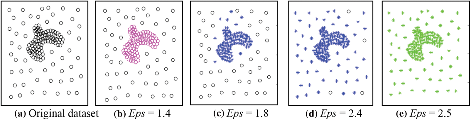
Figure 1: The results of DBSCAN using different values for Eps, MinPts = 4 for all

To solve the problem of clusters of varied densities, this article proposes a simple technique that allows DBSCAN to use suitable values for the Eps parameter, where each value is dedicated to a single density level. As a general case, a dataset that includes clusters of varied densities has the property that the number of objects in dense regions is more than that of objects in low-density areas. Thus, the proposed method can compute the value of Eps as the average of the core distances of all unclustered objects. Then it applies the traditional DBSCAN to the dataset to obtain clusters at the current density level. In the case of unclustered objects remaining, the proposed technique makes a new cycle to calculate a new value of Eps and applies the DBSCAN algorithm to the unclustered objects. Calculating the value of Eps in this manner removes it from the input parameters of the DBSCAN algorithm. So, the proposed technique requires only one input parameter. That means our contribution is discovering varied density clusters with minimal input parameters.

The problem with this research is the detection of clusters with different densities from the data. Many methods addressed this issue. Each method has its advantages and disadvantages. The methodology is as follows: This article reviews some techniques that addressed the problem to learn how to handle it and overcome their limitations and presents a proposed method to handle the issue. The proposed method depends on the traditional DBSCAN. This study evaluated the proposed method by applying it to many benchmark datasets. The results demonstrated the effectiveness of the proposed method. The accuracy of the method ranges from 92% to 100% for the experimented datasets.

This article is structured as follows: Section 2 reviews some related works. The proposed method is presented in Section 3. Section 4 introduces some experimental results that emphasize the ability of the proposed technique to discover clusters of varied densities. Section 5 concludes the article.

2  Related Works

Clustering has many useful features, making it one of the most well-known in many fields of image segmentation, pattern recognition, machine learning, data mining, etc. [12–16]. Clustering techniques aim to partition a dataset into subsets. Each subset includes similar objects, while dissimilar objects are assigned different subsets. Each subset is called a cluster. Density-based algorithms can discover clusters of different shapes and sizes but do not perform well in the presence of clusters of diverse densities. Thus, this part of the article mainly discusses some of the existing density-based algorithms.

Density-based methods do not require the number of clusters in advance. DBSCAN was the first algorithm proposed in this category. It considers clusters as dense regions separated from each other by low-density regions. Therefore, each cluster is a set of density-connected objects, and the dense objects are called cores. A core object has MinPts, at least in its neighborhood of fixed radius Eps. Objects that are not cores, but belong to the vicinity of any core, are called border objects. Objects that are neither cores nor borders are called noise objects. DBSCAN handles noise effectively. Therefore, it has been used for anomaly detection [17]. Since DBSCAN depends on two global parameters (Eps and MinPts), it fails to discover varied density clusters. Several methods have been proposed to overcome this problem. These methods may be classified into two categories: the first allows different values for Eps or Minpts, and the second uses alternative density definitions without Eps.

Many algorithms allow Eps to vary according to the local density of each region. In [18], the method finds the distance to the kth neighbor for each object and sorts the objects ascendingly based on these distances. Each cluster will have its own Eps value. The initial value of the Eps will be the distance to the kth neighbor of the first object in the sorted dataset, and the traditional DBSCAN is applied to the data using the present Eps value to get the first top dense cluster. The second top dense cluster will use the smallest kth distance among the unclassified objects as a new value for Eps then the DBSCAN is applied again. This process continues until all objects are clustered. This method produces several small clusters and may deliver singleton clusters.

In [19], the authors propose a method that allows the Eps and MinPts to vary from one iteration to the next. It starts with a random value for Eps. If the cluster size is below a threshold, the Eps is increased by 0.5. In addition, the method requires the number of clusters as an input, so this method is not suitable at all.

Multi-Density DBSCAN Cluster Based on Grid (GMDBSCAN) [20] divides the data space into grid cells of the same length, computes local MinPts for each grid cell according to its density, and applies the DBSCAN to each cell using the same Eps for all cells. This phase produces some sub-clusters, and the second phase merges the similar sub-clusters in the neighboring cells. This technique uses some computed thresholds that affect the final results. Using various local Minpts doesn’t guarantee to find clusters of diverse densities because Eps is constant for all cells. The other problem with GMDBSCAN is that it is time-consuming to perform well on massive datasets.

Multi-Density DBSCAN Cluster Based on Grid and Using Representative (GMDBSCAN-UR) [21] is a GMDBSCAN enhancement. It partitions data space into grid cells. But it selects representative objects from each cell and applies DBSCAN on each cell using local MinPts. Its running time is better than that of GMDBSCAN. But it doesn’t produce good results when the dataset includes clusters of varied densities.

Varied Density Based Spatial Clustering of Applications with Noise (VDBSCAN) [22] method selects appropriate Eps values from the k-dist plot, partitions the dataset into different levels of density then applies the DBSCAN on each density level using the proper value for Eps. This method produces good results when clusters are of different regular densities. If there is a gradient in density the result is not accurate.

DBSCAN algorithm based on Density Levels Partitioning (DBSCAN-DLP) [23] partitions the input dataset into different density level sets based on some statistical characteristic of density variation. Then estimates the Eps value for each density level set and applies DBSCAN clustering to each density level set with the corresponding Eps. This method is suitable for clusters of uniform density; the variance in the density of points in the same cluster should be tiny and less than a threshold.

In [24], the authors developed a mathematical concept to select different values for Eps from the k-dist plot and apply the DBSCAN algorithm to the data using the selected list of Eps values. They use spline cubic interpolation to find inflection points on the curve where the curve changes its concavity. This technique may divide some clusters since not all inflection points correspond to the correct different density levels.

Dominant Sets-DBSCAN (DSets-DBSCAN) [25] technique merges dominant sets clustering and DBSCAN. Initially, it runs DSets clustering, and from the resulting clusters, it determines the parameters for the DBSCAN algorithm. The former density-based clustering algorithms estimate the value of Eps based on some local density criteria and apply the DBSCAN to discover clusters from the dataset with multiple density levels.

Examples of algorithms that redefine the density are k-DBSCAN [26] and Multi Density DBSCAN [27]. k-DBSCAN [26] is a two-phase method. It assigns each object a local density value and then applies the k-means algorithm to cluster data objects based on their local densities. The result of this phase is a set of regions have different densities. In the second phase, it applies a modified version of DBSCAN to cluster data at each density level. The final result of this technique is highly dependent on the value of k used in k-means. k-DBSCAN needs more input parameters (l and k used in the k-means algorithm) than the DBSCAN algorithm, and the tuning parameters process is not an easy task.

Multi Density DBSCAN [27] method depends on two calculated parameters: 1-the average distance between each object and its k-nearest neighbors (DSTp). 2-the average distance between objects and their k-nearest neighbors in the cluster (AVGDST). This method permits tiny differences in density within the cluster. It uses sensitive threshold parameters to control the variance in density permitted within the cluster that affects the result.

K-deviation Density based DBSCAN (KDDBSCAN) [28] uses mutual k-nearest neighborhood to define the k-deviation density of an object and uses a threshold named density factor in place of Eps to get direct density reachable neighbors for core objects to expand the cluster.

Clustering Based on Local Density of Points (CBLDP) [29] algorithm discovers clusters of different densities. It depends on k-nearest neighbors and the density rank of each object. It classifies objects into attractors, attracted ones, and noises. A cluster consists of attractors and attracted objects (borders). It requires four input parameters, and that is a large number. Tuning these parameters is not always an easy task.

For each object, the Clustering Multi-Density Dataset (CMDD) [30] computes k values of local density. It sorts the data objects based on their local density to the kth neighbor, then starts the clustering process from the densest data object. It uses two parameters (MinPts and k), where k is used for k-nearest neighbors. It produces good clusters of different densities, but the denser cluster may take some objects from the adjacent low-dense cluster.

An Extended DBSCAN Clustering Algorithm (E-DBSCAN) [31] computes the local density of each object. Then it calculates the similarity between the data object and its k-nearest neighbors. If an object has MinPts similar data objects within its neighbors, then the data object is a core, and a cluster can be expanded from it. Otherwise, the data object is a noise temporarily. This method produces satisfactory results, but it requires three input parameters.

In [32], the authors propose a semi-supervised clustering method, which depends on DBSCAN. They partition the dataset into subsets of different levels of density based on the local density of each point in the dataset. Each subset contains points that have approximately the same density, where density variation is less than a threshold. Then, from each level of density, the method computes the parameters for DBSCAN to cluster the data at this level using them. The DBSCAN uses some knowledge given by an expert to monitor the growth of clusters.

Table 1 summarizes the advantages and disadvantages of similar methods.

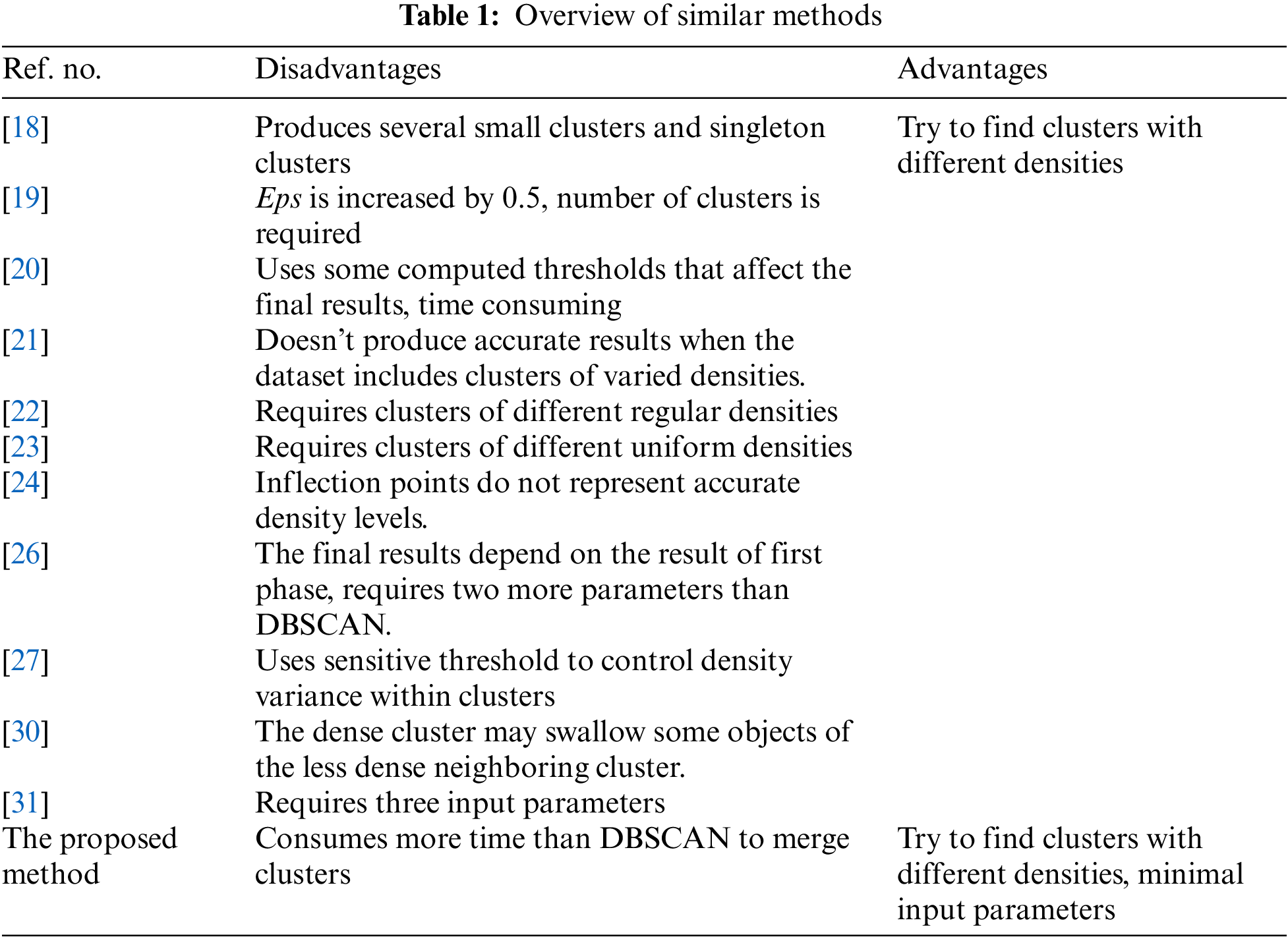
The proposed method requires MinPts as input only and calculates the appropriate values for Eps. It can find clusters of different densities even if there is no separation between them. However, this method requires more time than DBSCAN for merging clusters. Analytically, they have the same time efficiency O(n log n) using an index structure, such as R*-tree.

3  The Proposed Method (Adaptive DBSCAN)

This section presents the basic steps in the proposed method. The method assumes that each object in the dataset is a core object. A core object must have at least MinPts data objects within its neighborhood of radius Eps. So, it finds the smallest neighborhood radius for each object pi to be a core object. This distance is equal to the distance to the kth nearest neighbor of the object pi, where k equals MinPts. This distance is represented as coredistance(pi,MinPts).

The method depends on the DBSCAN algorithm, but it requires one input parameter only; this parameter is MinPts which is used in the same manner as in the traditional DBSCAN. This method computes an appropriate value for epsilon (Eps), as shown in (1). In (2), minEps is the minimum core distance over all the objects in the dataset.

Eps=1N∑i=1Ncoredistance(pi,MinPts)(1)

minEps=minimum distance(p,MinPts),minEps<>0(2)

After computing the Eps value, the method applies basic DBSCAN and obtains an initial result. Because anomalous objects in any dataset represent a small percentage of the dataset size, Eps may be less than the required value, and some clusters may need to be merged. For this reason, the method checks the border objects’ neighbors with objects in other clusters to see if the distance between them is less than or equal to Eps to merge them. Therefore, the method checks two neighboring clusters to combine them if possible. An object p is a border object if it has fewer than MinPts neighbors within its Eps neighborhood, but it belongs to the vicinity of a core object.

After that, there may be some noise objects inside a cluster. An object p is a noise object if it is neither a core nor a border object. A noise object that has a clustered neighbor x within Eps is assigned the same cluster of x. The following subfigures explain the idea; Fig. 2a represents the input dataset. Fig. 2b shows the result of applying the basic DBSCAN using the computed Eps on the input dataset. Where MinPts equals 12, and the calculated Eps is 17.964. The basic DBSCAN returns seven clusters, where the black circles are noises. You see that the computed value of Eps as in (1) is less than the required. So, the method merges the smaller cluster with its neighboring cluster if any border object has a neighbor object from the other cluster within the computed Eps distance. After fixing this problem, the result is as in Fig. 2c. You see two noise objects within the green cluster and one noise object at the border of the red cluster in Fig. 2c. If the distance between any noise object (the object is noise according to the current value of Eps) and its closest clustered neighbor is less than Eps, then the noise object is assigned to the cluster of that neighbor. After assigning noise objects to the nearest clusters, the result is as in Fig. 2d. At this point of computation, the first level of clustering is finished.

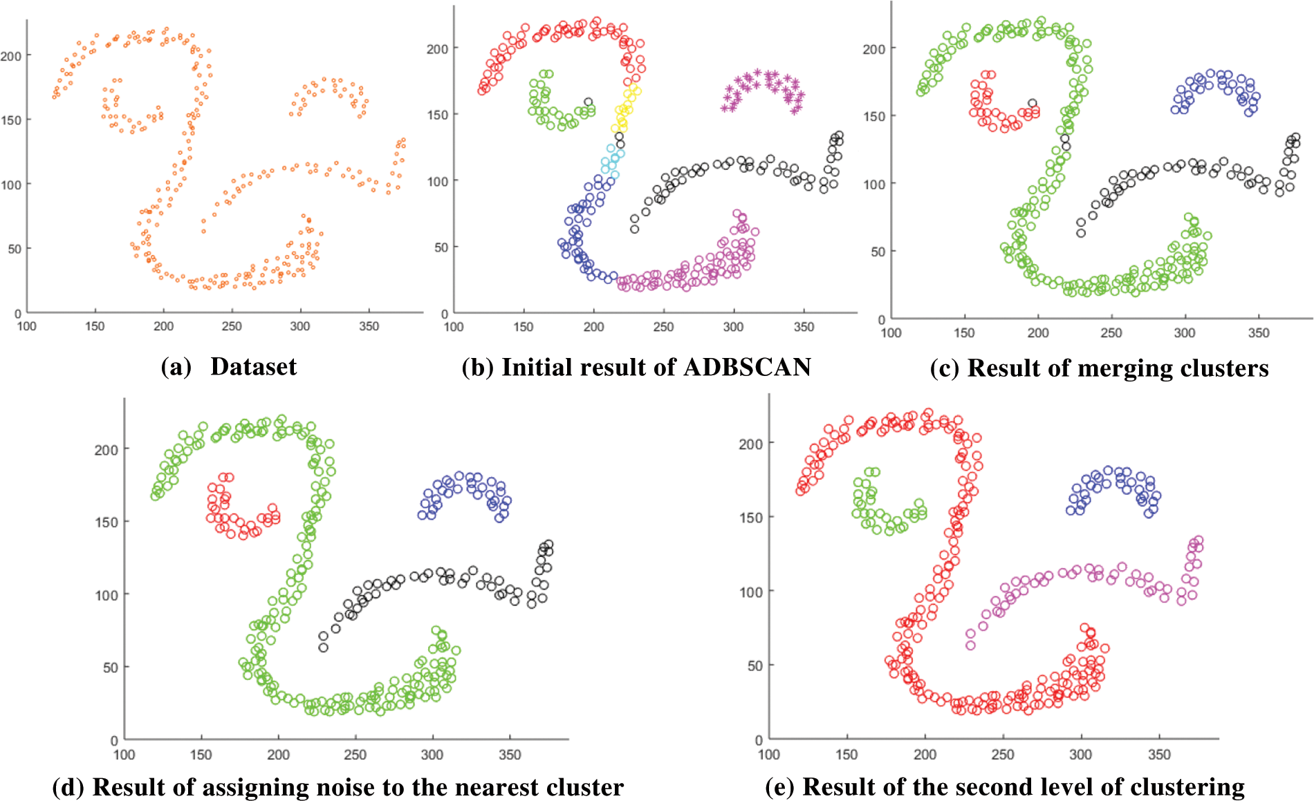
Figure 2: Result of the proposed method

In Fig. 2d, the black circular objects are noise according to the value of Eps. These noise objects are treated as unclustered objects in the next iteration, a new value of the Eps is computed as the average distance to the MinPts-neighbor of all noise objects as in (3), where minEps is calculated as in (2), and m refers to the number of noise objects (unclustered objects).

Eps=minEps+1m∑i=1mcoredistance(pi,MinPts)(3)

After computing the new value of Eps, the method applies the basic DBSCAN again, ignoring the clustered objects, and uses the fix procedure as in the previous level. Fig. 2e shows the result that represents the final result since no noise objects (unclustered) are remaining. In the case of noise objects remaining (treated as unclustered objects), the method moves to the next level of clustering until all objects are clustered, or noise objects (unclustered objects) are less than 0.006 of the size of the dataset. 0.006 of dataset size is a tiny portion of the dataset, and the final fix procedure tries to assign noise objects to the nearest cluster if possible.

After that, the method applies the final fix procedure, which performs the following tasks: It tries to merge nearby clusters if possible, assigns noise objects to the nearest cluster if possible, and tries to combine small clusters if there are no noise objects in the dataset. Specifically, if the cluster size is smaller than double MinPts, it attempts to merge it with the nearest cluster if possible. In this case, the smaller cluster will be merged with the nearest one if the distance between them is less than the average of the Eps values used in each of them. Any cluster that has fewer than MinPts objects is considered noise.

The proposed method works as described in the following steps:

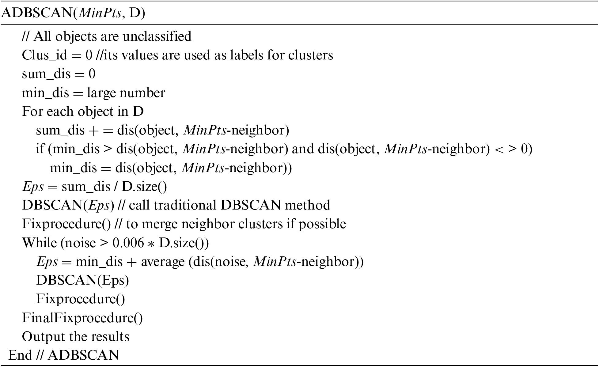
The ADBSCAN (MinPts, D) sketches the main steps of the proposed algorithm, which computes the initial value of Eps and calls the function DBSCAN(Eps) to get the densest clusters from the dataset. After that, it calls the function Fixprocedure() to fix the problem of using a small Eps value. When the dataset contains un-clustered objects (noise) that are more than 0.006 of its size, the method moves to the next level of density by computing a new Eps value and calling the DBSCAN(Eps) and Fixprocedure() functions. Finally, it calls FinalFixprocedure() to get the final result and outputs it.

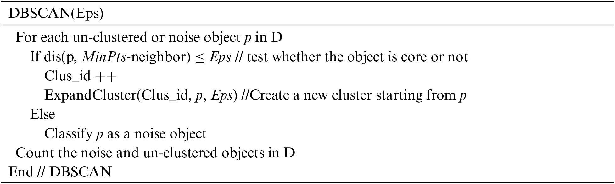
The DBSCAN (Eps) function performs the clustering process using the computed Eps. When calling this function for the first time, all objects are unclustered. But for subsequent calls, unclustered objects are assigned noise. If the object p is core according to Eps, the function creates a new label for the new cluster and starts to expand it by calling the ExpandCluster(Clus_id, p, Eps) function.

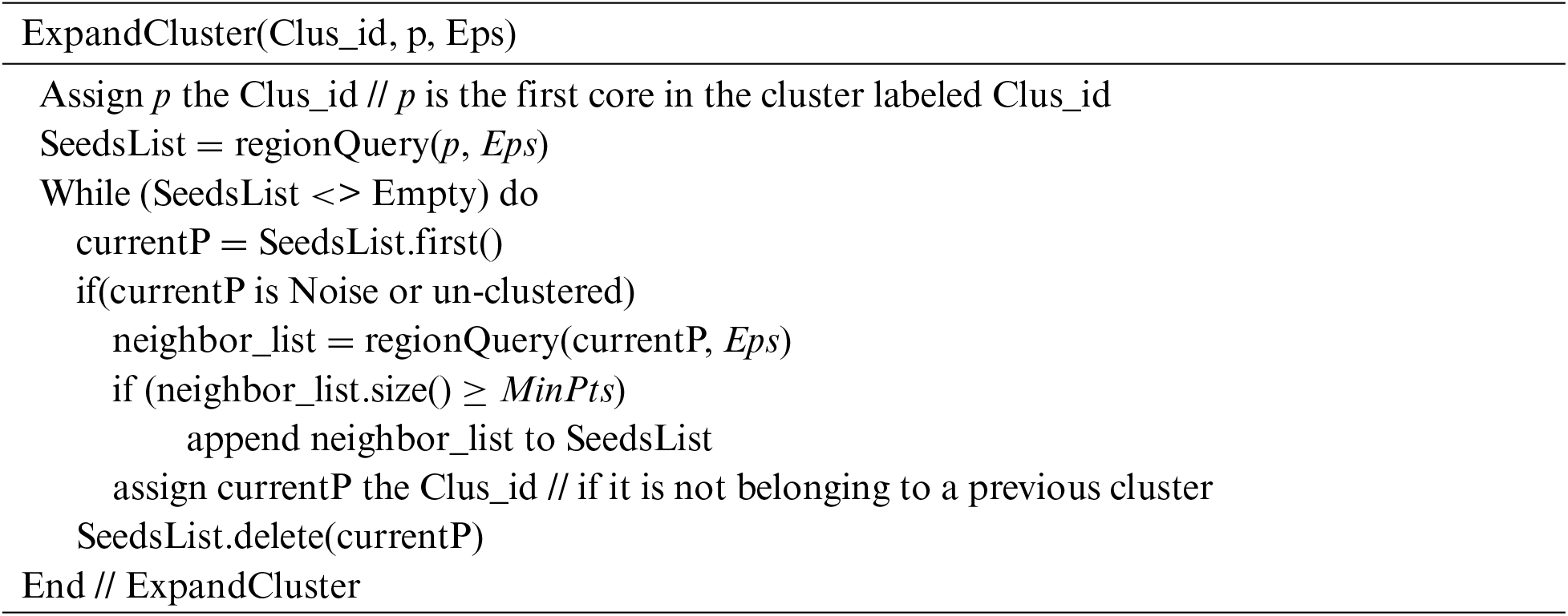
The ExpandCluster (Clus_id, p, Eps) function starts the cluster from the first core object p. It finds p’s neighbors in Eps distance. These neighbors are the borders and cores. So, it checks every p’s neighbor (that does not belong to any discovered cluster) to test whether it is a border or a core object. If it is a border object, the function assigns it to the current cluster. Otherwise, the function finds its neighbors and adds them to the SeedsList, then assigns the object to the current cluster. This process continues until the SeedsList is empty and the control backs to the DBSCAN(Eps) function.

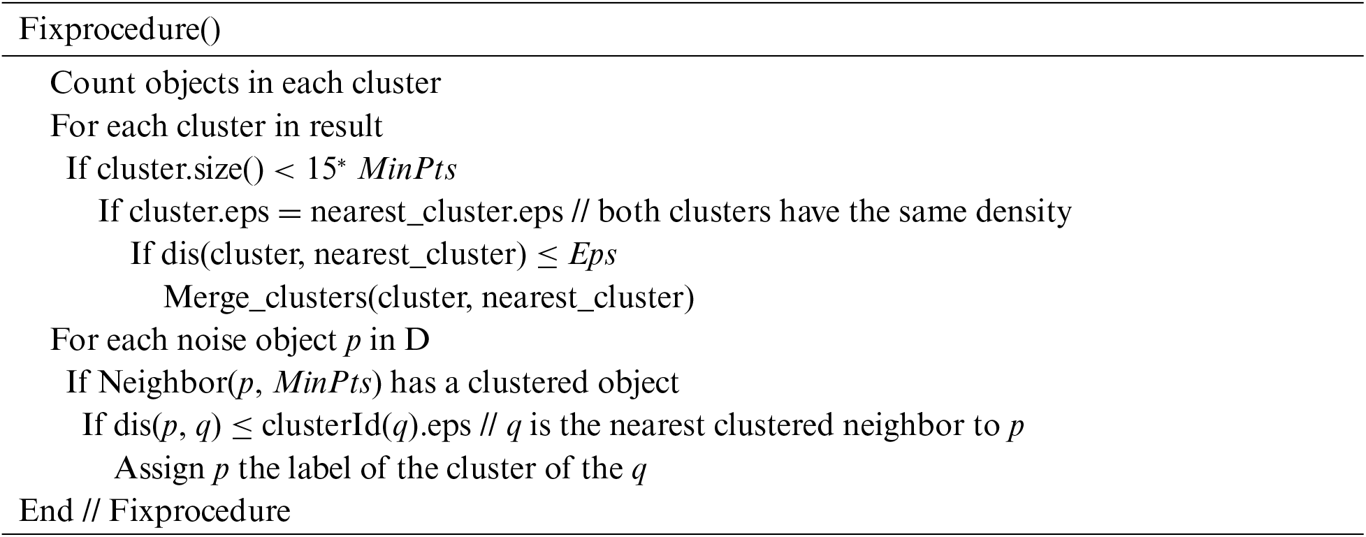
The Fixprocedure () function tries to merge the close clusters of the same density. This function solves the problem of using a small Eps value. Also, it assigns any noise object that has a clustered object x within its Eps neighborhood the same cluster of x.

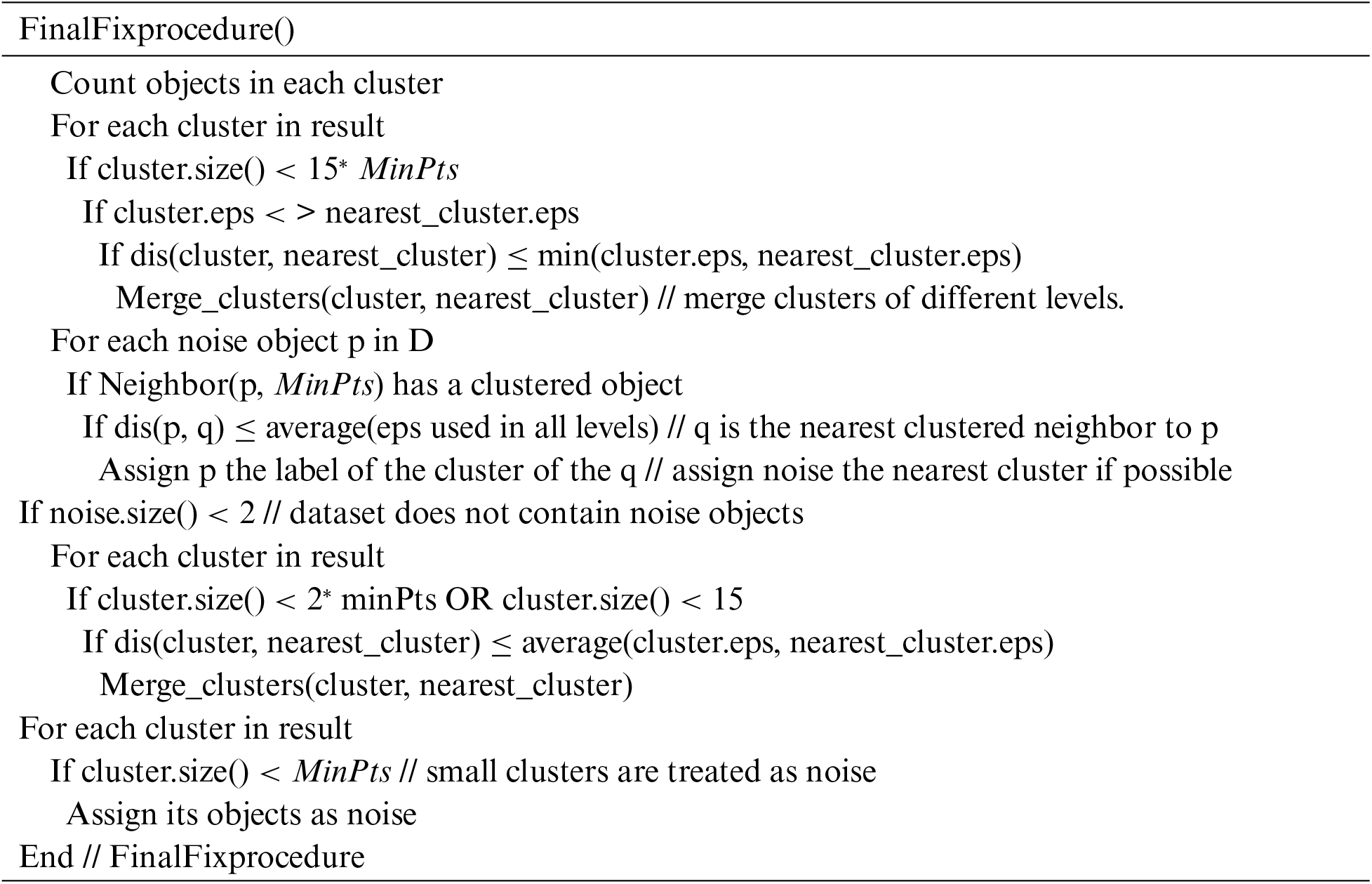
Using the FinalFixprocedure() function is practical, especially when the dataset doesn’t contain noise. The method tries to merge clusters created using different Eps values such that the distance between them is less than the lowest Eps value. After that, it assigns noise objects to their nearest cluster using the average value of all the Eps values used in all density levels. Then it merges the tiny clusters to their nearest clusters using the average value of all the Eps values used through all density levels. Finally, any cluster that has fewer objects than MinPts is treated as noise by assigning its objects to noise.

4  Experimental Results

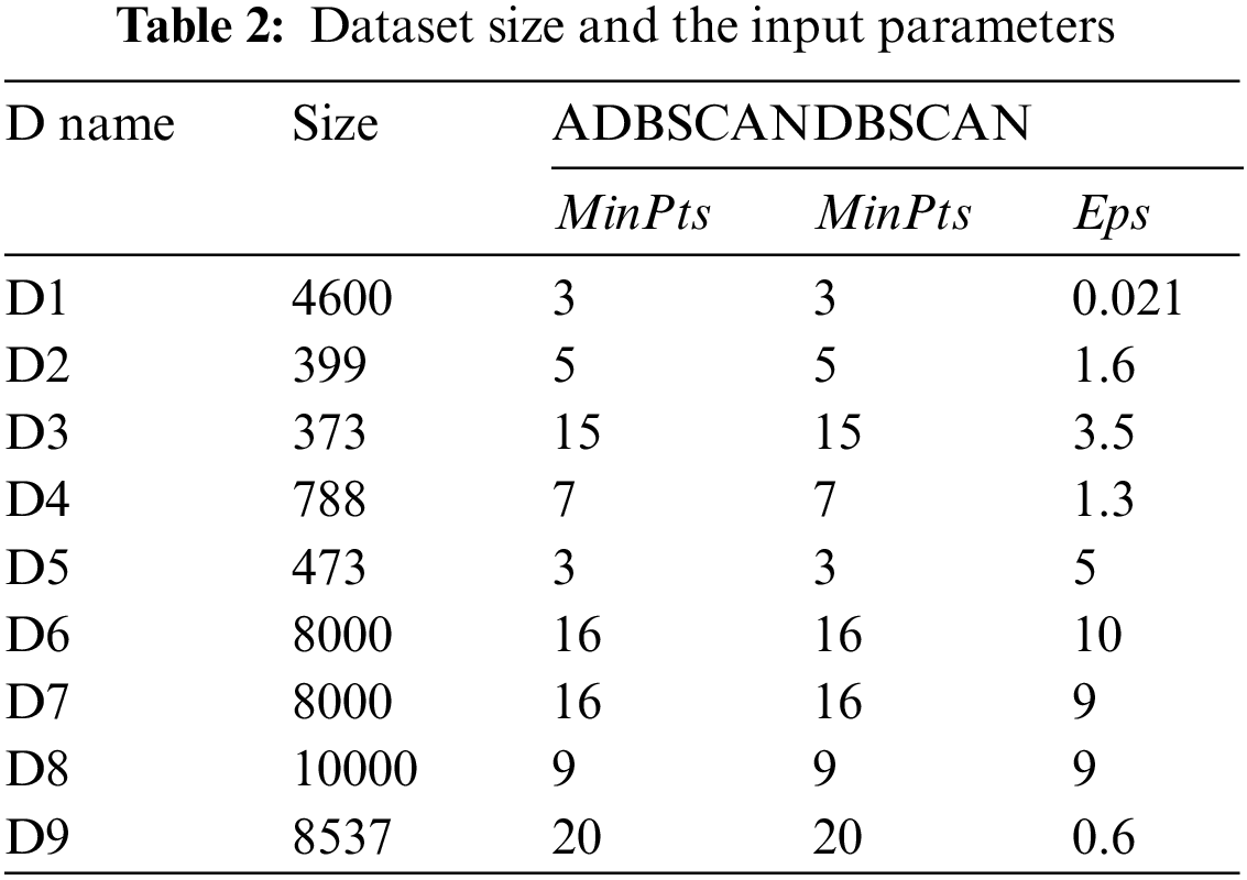
This section demonstrates the results of applying the proposed method ADBSACN on some datasets, which show its superior ability to discover clusters of different densities. Table 2 shows the size of each dataset and the used parameters with their values. Note that MinPts is the same for DBSCAN and the proposed method (ADBSCAN). All datasets are of two-dimensional space for the sake of clarity. The code is written using C++ and has been run on a dell laptop with 6 GB RAM and an Intel(R) Core (TM) i5 CPU @ 2.50 GHz. The computer runs the Windows 10 Home Edition operating system.

The first dataset, D1, has two levels of density where the high-density cluster separates the low-density one into two clusters, as shown in Fig. 3a. The result of the proposed method is shown in Fig. 3b, where it discovers the three clusters, while DBSCAN fails to find the correct clusters using a single value for Eps, as shown in Fig. 3c.

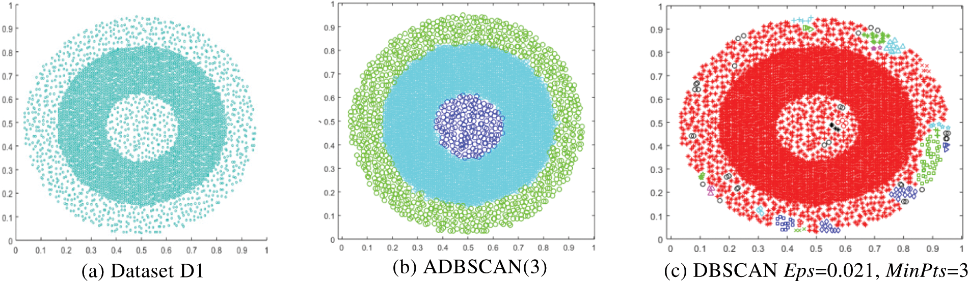
Figure 3: Dataset D1 and the result of using ADBSCAN and DBSCAN

The second dataset, D2, is a compound dataset. It has multiple levels of density, as shown in Fig. 4a. The ADBSCAN discovers seven clusters, as shown in Fig. 4b, while DBSCAN fails to locate the correct clusters, as shown in Fig. 4c, where it returns the low-density cluster as noise and treats some border objects as noise. Fig. 4d shows the result of DBSCAN where it merges the two left bottom clusters and treats the low-density cluster as noise, represented by black circles.

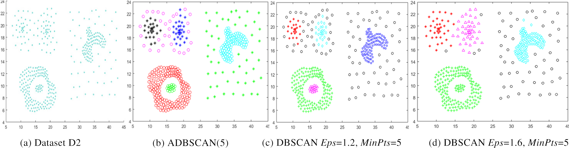
Figure 4: Dataset D2 and the result of using ADBSCAN and DBSCAN

The third dataset, D3, contains two clusters of different densities, as shown in Fig. 5a. The ADBSCAN discovers the two clusters, as shown in Fig. 5b, while the DBSCAN fails to find them, as shown in Fig. 5c, where it divides the low-density cluster into two subclusters and merges one of them with the high-density cluster and treats some objects as noise, represented by black circles.

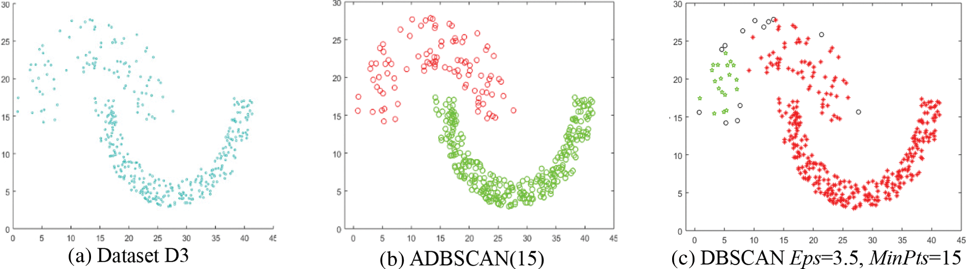
Figure 5: Dataset D3 and the result of using ADBSCAN and DBSCAN

The fourth dataset, D4, has seven clusters, as shown in Fig. 6a. Without using the FinalFixProcedure(), the ADBSCAN finds two density levels; it finds eight clusters, with the crescent cluster returning as two clusters, as shown in Fig. 6b. But using the FinalFixprocedure(), the proposed method returns seven clusters, as shown in Fig. 6c. The DBSCAN finds seven clusters also. It treats some objects as noise, as shown in Fig. 6d. The noise is represented by black circles.

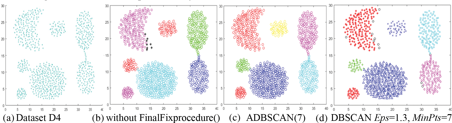
Figure 6: Dataset D4 and the result of using ADBSCAN and DBSCAN

The fifth dataset, D5, contains multiple levels of density. It has eight clusters and some noise objects, as shown in Fig. 7a. Without using the FinalFixprocedure() function, the proposed method returns ten clusters, where one of them contains two objects (blue stars at the top left), as shown in Fig. 7b. But it discovers eight clusters after using the FinalFixprocedure(). It merges the blue circles cluster with the green stars cluster. They were discovered using different values of Eps. The blue stars cluster is treated as noise because of its low density and inability to merge with the nearest cluster, Fig. 7c depicts this outcome. The DBSCAN cannot discover these clusters, as shown in Fig. 7d, where it returns the lowest density cluster as noise and merges the four clusters on the right side of Fig. 7d. Discovering these clusters using the traditional DBSCAN is impossible.

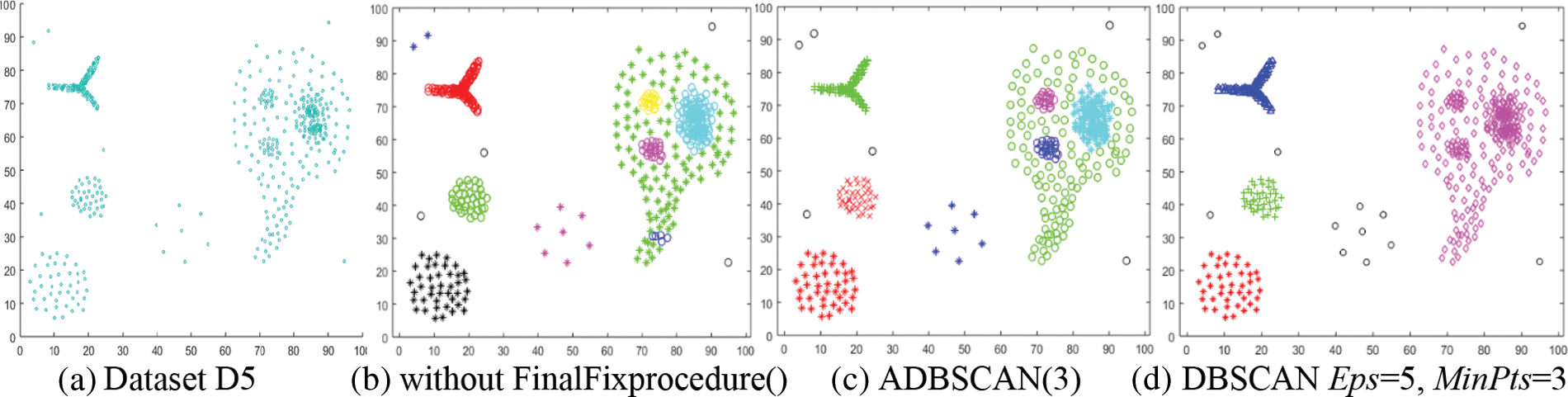
Figure 7: Dataset D5 and the result of using ADBSCAN and DBSCAN

The sixth dataset, D6, has six clusters with chains of objects that connect some of them, as shown in Fig. 8a. The proposed method returns the main six clusters in addition to four small clusters that will be treated as noise when applying the FinalFixprocedure(). The chains are returned as four clusters, as shown in Fig. 8b. The final result of the proposed method treats the four small clusters as noise, represented by black circles, as shown in Fig. 8c. The DBSCAN returns the main six clusters and three small clusters, but it also returns several noise objects represented by black circles, as shown in Fig. 8d.

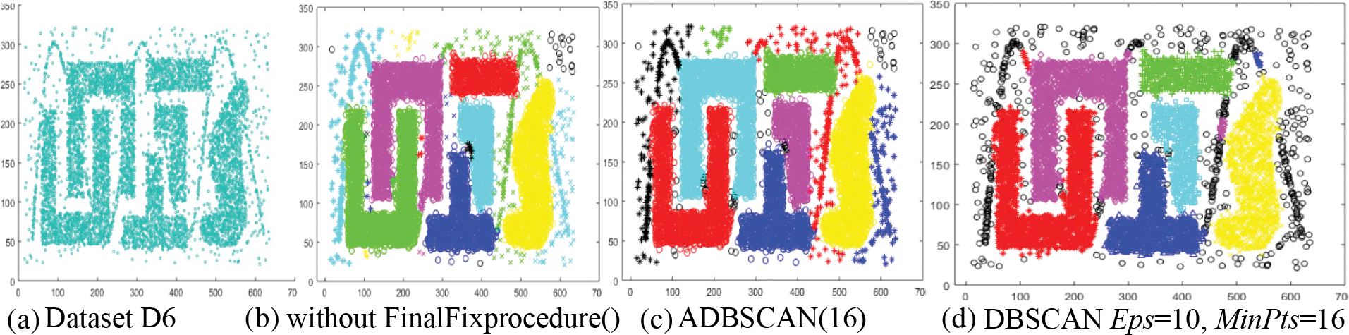
Figure 8: Dataset D6 and the result of using ADBSCAN and DBSCAN

The seventh dataset, D7, contains six high-density clusters, and a chain of dense objects connects them. These clusters are placed within a low-density region, as shown in Fig. 9a. Without applying the FinalFixprocedure(), the proposed method returns the main six clusters and five small clusters, in addition to six clusters from the low-density region, as shown in Fig. 9b. The final result of the ADBSCAN is shown in Fig. 9c, where it treats the five small clusters as noise. The DBSCAN returns good results where it discovers the main six clusters and treats the low-density region as noise, as shown in Fig. 9d. The black circles represent the noise objects.

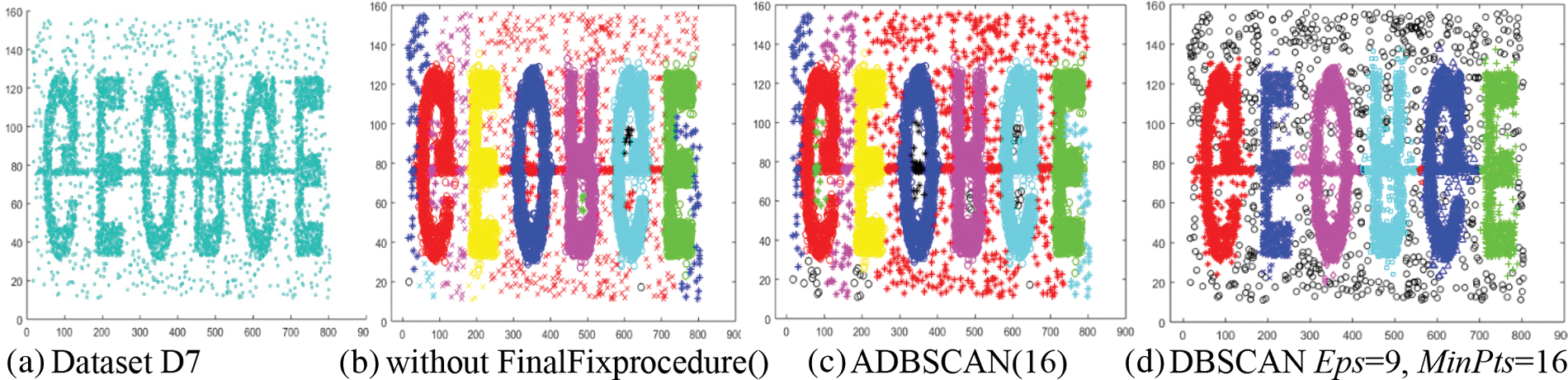
Figure 9: Dataset D7 and the result of using ADBSCAN and DBSCAN

The eighth dataset, D8, contains nine clusters of the same density, as shown in Fig. 10a. Even without using FinalFixprocedure(), the proposed method finds the nine clusters and some small clusters shown in Fig. 10b. The final result of ADBSCAN is shown in Fig. 10c, where it treats small clusters as noise. DBSCAN returns the nine main clusters in addition to three small clusters and numerous noise objects, as shown in Fig. 10d.

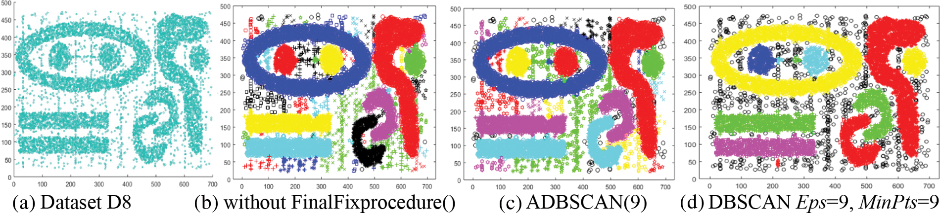
Figure 10: Dataset D8 and the result of using ADBSCAN and DBSCAN

The ninth dataset, D9, contains clusters of different densities, as shown in Fig. 11a. The proposed method returns better results than that of DBSCAN. The proposed method returns ten clusters, as shown in Fig. 11b. When the FinalFixprocedure() is used, small clusters are treated as noise, as illustrated in Fig. 11c, where the noise is represented by the black circle. As shown in Fig. 11d, DBSCAN treats several objects from the two clusters on the left side as noise.

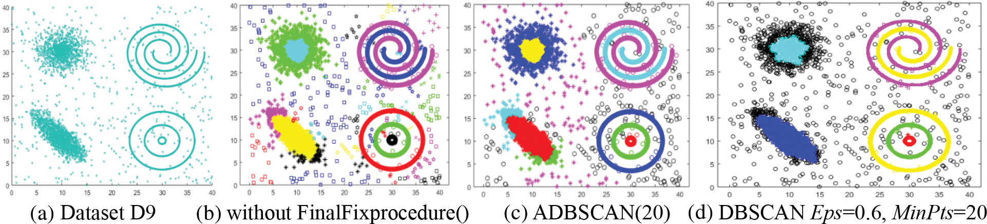
Figure 11: Dataset D9 and the result of using ADBSCAN and DBSCAN

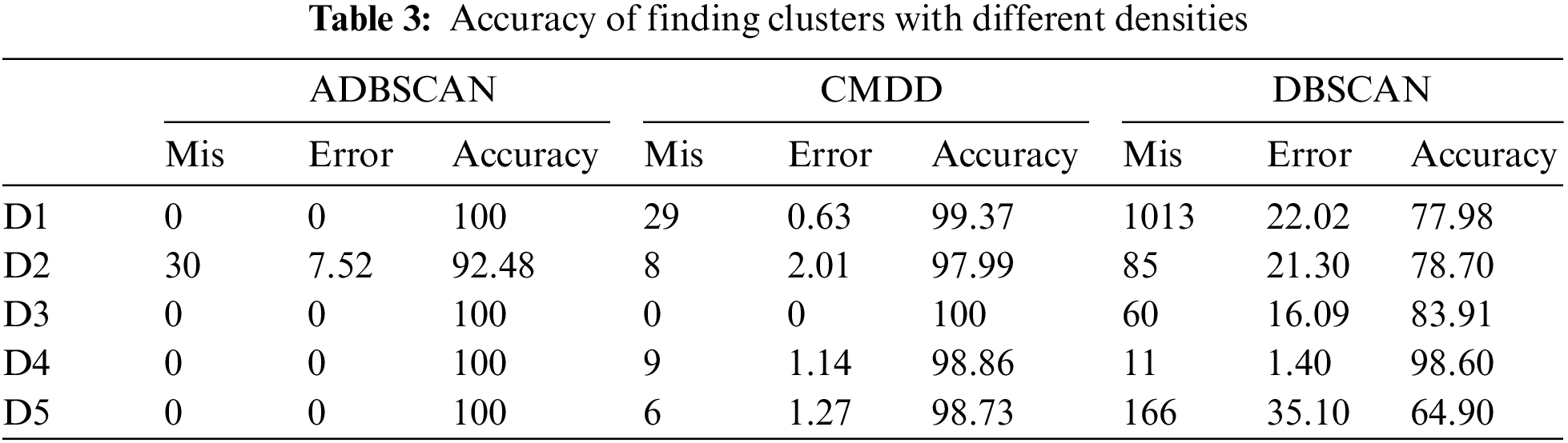
Fig. 12 shows the results of applying the CMDD algorithm to datasets. Comparing the output of CMDD with that of ADBSCAN and DBSCAN of the same datasets presented through figures from Figs. 3 to 11, ADBSCAN produces better clusters than DBSCAN and CMDD. Table 3 shows the misclassified objects for each method and each dataset. The percentage of error is computed as in (4). The accuracy is computed as in (5). The results show that the proposed method can effectively find clusters of different densities.

percentage of error =Number of miss clustered objectsSize of the dataset∗100(4)

accuracy =100−percentage of error (5)

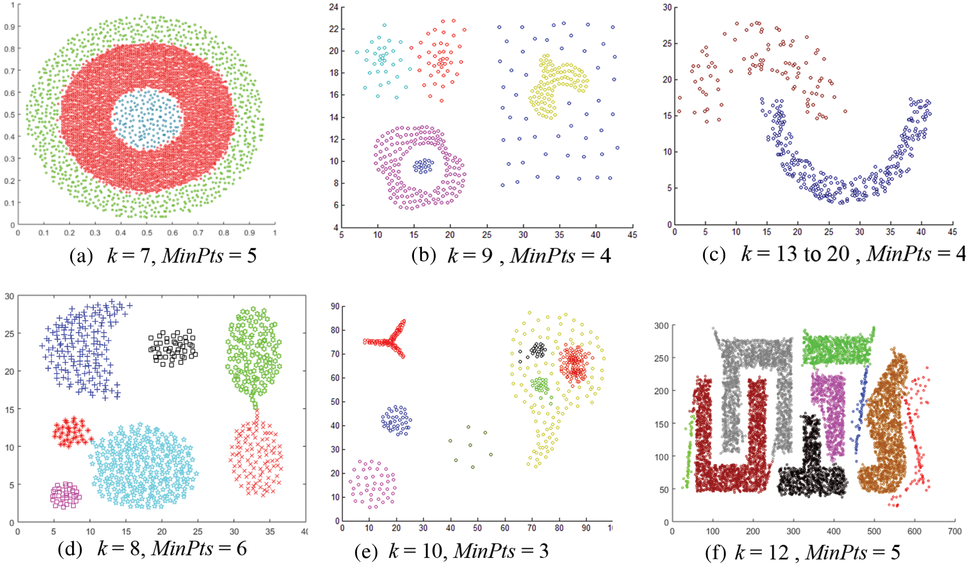
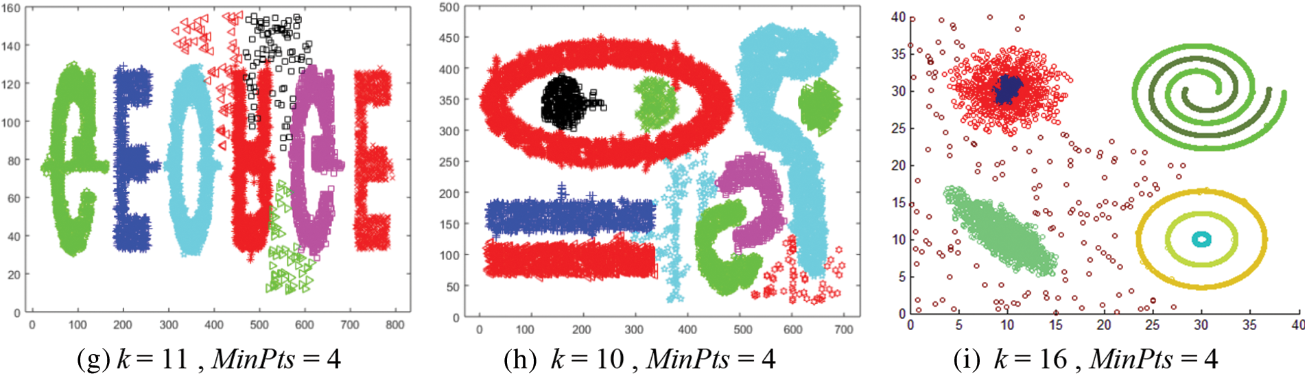
Figure 12: Results of applying the CMDD algorithm to datasets

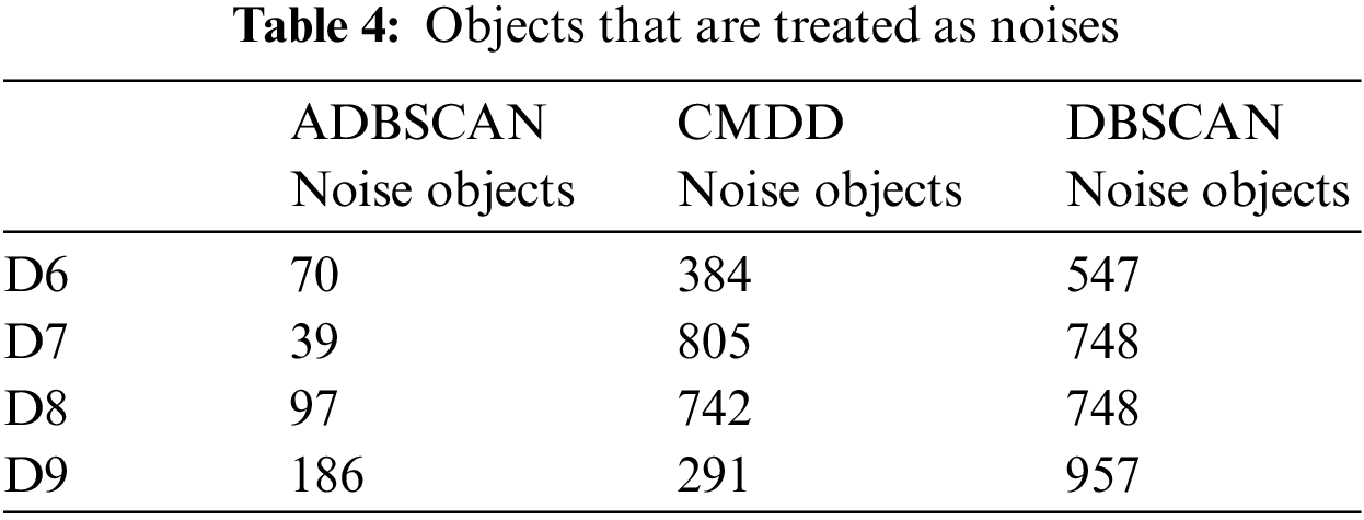
For datasets from D6 to D9, there is no exact clustering solution to compare the output of the studied methods with it. So, Table 4 presents the number of noise objects. Note that the proposed method returns a minimal number of noise objects.

5  Conclusion

This paper introduces an adapted version of the DBSCAN clustering algorithm. DBSCAN is a density-based method that can discover clusters of varied shapes and sizes and handle noise well. However, its main problem is its inability to find clusters of various densities furthermore the sensitivity of its parameter called Eps. The quality of the result depends on the success of selecting a suitable value for the Eps parameter.

The proposed method introduces a simple way to set the Eps value according to the density of unclassified objects in the dataset. Eps is the average distance to the MinPts-neighbor of unclassified data objects. This method reduces the required input parameters for DBSCAN and raises its ability to discover different density clusters. The experimental results prove that the proposed method successfully finds varied density clusters. However, the proposed method consumes more time than DBSCAN to merge clusters. Analytically, they have the same time efficiency O(n log n) using an index structure, such as R*-tree.

Funding Statement: The author extends his appreciation to the Deputyship for Research & Innovation, Ministry of Education in Saudi Arabia for funding this research work through the project number (IF-PSAU-2021/01/17758).

Conflicts of Interest: The authors declare that they have no conflicts of interest to report regarding the present study.

References

1. R. T. Ng and J. Han, “CLARANS: A method for clustering objects for spatial data mining,” IEEE Transactions on Knowledge and Data Engineering, vol. 14, no. 5, pp. 1003–1016, 2002. [Google Scholar]

2. A. Fahim, “K and starting means for k-means algorithm,” Journal of Computational Science, vol. 55, no. October, pp. 101445, 2021. [Google Scholar]

3. A. A. Sewisy, M. H. Marghny, R. M. Abd ElAziz and A. I. Taloba, “Fast efficient clustering algorithm for balanced data,” International Journal of Advanced Computer Science and Applications, vol. 5, no. 6, pp. 123–129, 2014. [Google Scholar]

4. T. Zhang, R. Ramakrishnan and M. Livny, “BIRCH: An efficient data clustering method for very large databases,” ACM SIGMOD Record, vol. 25, no. 2, pp. 103–114, 1996. [Google Scholar]

5. S. Guha, R. Rastogi and K. Shim, “Cure: An efficient clustering algorithm for large databases,” ACM SIGMOD Record, vol. 27, no. 2, pp. 73–84, 1998. [Google Scholar]

6. M. Ester, H. -P. Kriegel, J. Sander and X. Xiaowei, “A density-based algorithm for discovering clusters in large spatial databases with noise,” in Proc. of KDDM, Portland, USA, pp. 226–231, 1996. [Google Scholar]

7. Y. Chen, L. Zhou, N. Bouguila, C. Wang, Y. Chen et al., “BLOCK-DBSCAN: Fast clustering for large scale data,” Pattern Recognition, vol. 109, no. January, pp. 107624, 2021. [Google Scholar]

8. R. Zhang, H. Peng, Y. Dou, J. Wu, Q. Sun et al., “Automating DBSCAN via deep reinforcement learning,” in Proc. of CIKM, Atlanta, Georgia, USA, pp. 2620–2630, 2022. [Google Scholar]

9. Q. Hu and Y. Gao, “A Novel clustering scheme based on density peaks and spectral analysis,” in Proc. of ISSSR, Chongqing, China, pp. 126–132, 2021. [Google Scholar]

10. A. Hinneburg and D. A. Keim, “An efficient approach to clustering in large multimedia databases with noise,” in Proc. of KDDM, New York, NY, USA, pp. 58–65, 1998. [Google Scholar]

11. W. Wang, J. Yang and R. Muntz, “STING: A statistical information grid approach to spatial data mining,” in Proc. of VLDB, Athens, Greece, pp. 186–195, 1997. [Google Scholar]

12. R. Kuo and F. E. Zulvia, “Automatic clustering using an improved artificial bee colony optimization for customer segmentation,” Knowledge and Information Systems, vol. 57, no. 2, pp. 331–357, 2018. [Google Scholar]

13. S. S. Nikam, “A comparative study of classification techniques in data mining algorithms,” Oriental Journal of Computer Science & Technology, vol. 8, no. 1, pp. 13–19, 2015. [Google Scholar]

14. A. Alrosan, W. Alomoush, M. Alswaitti, K. Alissa, S. Sahran et al., “Automatic data clustering based mean best artificial bee colony algorithm,” Computers, Materials & Continua, vol. 68, no. 2, pp. 1575– 1593, 2021. [Google Scholar]

15. E. H. Houssein, K. Hussain, L. Abualigah, M. Abd Elaziz, W. Alomoush et al., “An improved opposition-based marine predators algorithm for global optimization and multilevel thresholding image segmentation,” Knowledge-Based Systems, vol. 229, no. 1, pp. 107348, 2021. [Google Scholar]

16. A. I. Taloba, A. A. Sewisy and Y. A. Dawood, “Accuracy enhancement scaling factor of viola-jones using genetic algorithms,” in Proc. of ICENCO, Cairo, Egypt, pp. 209–212, 2018. [Google Scholar]

17. P. Jain, M. S. Bajpai and R. Pamula, “A modified DBSCAN algorithm for anomaly detection in time-series data with seasonality,” The International Arab Journal of Information Technology, vol. 19, no. 1, pp. 23–28, 2022. [Google Scholar]

18. A. Fahim, “Homogeneous densities clustering algorithm,” International Journal of Information Technology and Computer Science, vol. 10, no. 10, pp. 1–10, 2018. [Google Scholar]

19. M. M. R. Khan, M. A. B. Siddique, R. B. Arif and M. R. Oishe, “ADBSCAN: Adaptive density-based spatial clustering of applications with noise for identifying clusters with varying densities,” in Proc. of iCEEiCT, Dhaka, Bangladesh, pp. 107–111, 2018. [Google Scholar]

20. C. Xiaoyun, M. Yufang, Z. Yan and W. Ping, “GMDBSCAN: Multi-density DBSCAN cluster based on grid,” in Proc. of ICEBE, Xi’an, China, pp. 780–783, 2008. [Google Scholar]

21. M. A. Alhanjouri and R. D. Ahmed, “New density-based clustering technique: GMDBSCAN-UR,” International Journal of Advanced Research in Computer Science, vol. 3, no. 1, pp. 1–9, 2012. [Google Scholar]

22. P. Liu, D. Zhou and N. Wu, “Varied density based spatial clustering of application with noise,” in Proc. of ICSSSM, Chengdu, China, pp. 528–531, 2007. [Google Scholar]

23. Z. Xiong, R. Chen, Y. Zhang and X. Zhang, “Multi-density DBSCAN algorithm based on density levels partitioning,” Journal of Information & Computational Science, vol. 9, no. 10, pp. 2739–2749, 2012. [Google Scholar]

24. S. Louhichi, M. Gzara and H. Ben Abdallah, “A density based algorithm for discovering clusters with varied density,” in Proc. of WCCAIS, Hammamet, Tunisia, pp. 1–6, 2014. [Google Scholar]

25. J. Hou, H. Gao and X. Li, “DSets-DBSCAN: A parameter-free clustering algorithm,” IEEE Transactions on Image Processing, vol. 25, no. 7, pp. 3182–3193, 2016. [Google Scholar] [PubMed]

26. M. Debnath, P. K. Tripathi and R. Elmasri, “K-DBSCAN: Identifying spatial clusters with differing density levels,” in Proc. of DMIA, San Lorenzo, Paraguay, pp. 51–60, 2015. [Google Scholar]

27. W. Ashour and S. Sunoallah, “Multi density DBSCAN,” Lecture Notes in Computer Science (including Subser. Lect. Notes Artif. Intell. Lect. Notes Bioinformatics), vol. 6936, pp. 446–453, 2011. [Google Scholar]

28. C. Jungan, C. Jinyin, Y. Dongyong and L. Jun, “A k-deviation density based clustering algorithm,” Mathematical Problems in Engineering, vol. 2018, no. 10, pp. 1–16, 2018. [Google Scholar]

29. A. Fahim, “A clustering algorithm based on local density of points,” International Journal of Modern Education and Computer Science, vol. 9, no. 12, pp. 9–16, 2017. [Google Scholar]

30. A. Fahim, “Clustering algorithm for multi-density datasets,” Romanian Journal of Information Science and Technology, vol. 22, no. 3–4, pp. 244–258, 2019. [Google Scholar]

31. A. Fahim, “An extended DBSCAN clustering algorithm,” International Journal of Advanced Computer Science and Applications, vol. 13, no. 3, pp. 245–258, 2022. [Google Scholar]

32. A. A. Almazroi and W. Atwa, “An improved clustering algorithm for multi-density data,” Axioms, vol. 11, no. 8, pp. 411, 2022. [Google Scholar]