Metaheuristic Optimization with Deep Learning Enabled Smart Grid Stability Prediction

1  Introduction

Smart Grid (SG) is a system that enables device to interact with consumer and supplier. SG’s aim is to compute the optimal generator-communication-distribution pattern, reduce cost, and save energy [1]. Electricity prediction performs a vital role in SG [2]. The popular task in SG is to predict electricity. Precise predicting assistances in scheduling reasonably the electrical generators, that is advantageous for saving electric power and reducing production cost [3]. Because of deregulated electrical energy market, the dynamics of electrical energy trade are totally unrelated. Electricity covers a set of faces i.e., uncommon to alternate markets like load are associated with environmental factors such as unexpected price peaks, weather conditions. Electricity became a centralized study field in energy because of its distinct behaviours. Electricity prediction is the major problem confronted by market participants and electricity market is built to create grid stability. Through ambiguous prediction, the steadiness of grid compromised and increase the blackout risk [4]. Fig. 1 illustrates the framework of smart grid.

Figure 1: Structure of smart grid

Timely and accurate transmission of state of distribution, generation, and transmission system is crucial to ensure the steadiness of connected smart electrical power grids [5]. The failure in SA mainly happened because of insufficient data shared over controller region, leading to cascading blackout. A smart system increases the ability to understand, plan, learning difficulty, to take proper action to guarantee stability are desired, and to share understanding over adjacent areas. A smart grid could forecast the electricity demand as the requirement of the hour. This is attained by the application of Machine Learning (ML) algorithm [6] on the information produced from the grid. The smarter grid could assist in reducing pollution and makes the power cost very cheap. ML resembles a method for handling considerable amount of information in an electrical grid. It provides a systematic manner for making proper decisions to operate the grid and analyze the information.

ML functionality includes power production, fault detection, future optimal scheduling during data breach, price, and load prediction [7]. ML models focused on constructing programs that learn from experience. The objective of ML models is to offer automated data to learn from new information which is utilized in the decision-making method for implementing innovative prediction methods [8]. Furthermore, ML has alienated into four classes: Reinforcement Learning (RL) algorithm, Supervised (SL) approach, Unsupervised-Learning (UL) approach, and Semi-Supervised-Learning (SSL) approach. SL algorithm trained on labelled information, but each information is unlabelled in UL. In SSL algorithm, few information is labelled, and major information is unlabelled, whereas RL algorithm learns via delayed feedback by communicating with environments [9]. DL is a subdivision of ML model. It is a familiar subset of ML because of its exclusive capacity. In ML model, designer automatically alters, when ML model provides inaccurate predictions; but, DL approach concludes manually when prediction is accurate or not [10].

This article introduces a new Social Spider Optimization with Deep Learning Enabled Statistical Analysis for Smart Grid Stability (SSODLSA-SGS) prediction model. Primarily, class imbalance data handling process is performed using Synthetic minority oversampling technique (SMOTE) technique. The SSODLSA-SGS model derives a deep belief-back propagation neural network (DBN-BN) model for the prediction of SG stability. Moreover, social spider optimization (SSO) algorithm can be applied for determining the optimal hyperparameter values of the DBN-BN model. The design of SSO algorithm helps to appropriately modify the hyperparameter values of the DBN-BN model. A series of simulation analyses are conducted to highlight the enhanced outcomes of the SSODLSA-SGS algorithm.

2  Related Works

In [11], many recent ML techniques such as SVM, KNN, LR, NB, NN, and DT classification are utilized for forecasting the stability of SG. The SG data set utilized from the study was publicly obtainable gathered in UC Irvine (UCI) ML repository. In [12], an SG with intelligent system was being utilized for catering the dynamic power requirement. An SG model follows the Cyber-Physical System (CPS), whereas Information Technology (IT) framework was combined with physical system. During this condition of the SG embedding with CPS, the ML component is the IT aspects and the power dissipation unit is the physical entity. During this study, a novel Multidirectional LSTM (MLSTM) approach was being presented for predicting the stability of SG networks. Massaoudi et al. [13] designed a DL algorithm based BiGRU to SG stability forecast. In order to automatic tune, this analysis utilized Simulated Annealing (SA) technique for optimizing the chosen hyperparameter and improving the model predictability. The presented prediction model performance was estimated utilizing electric grid stability simulating dataset.

Breviglieri et al. [14] introduced optimizing DL techniques for solving set inputs (variables of formulas) and equality problems from DSGC system. So, the measure the grid frequency of all customers are served for providing the network administrator with each needed data on the existing network power balance, and so it is price their energy offering—and inform consumer—consequently. Rodríguez et al. [15] progress a novel method to predict photovoltaic generator outcome power confidence interval 10 min ahead, dependent upon DL, mathematical probability density functions (PDF), and meteorological parameters.

3  The Proposed Model

In the study, a new SSODLSA-SGS algorithm has been developed is to determine the stability level in the SGs. The proposed SSODLSA-SGS technique comprises of SMOTE based class imbalance data handling, data pre-processing (data normalization and transformation), DBN-BN based prediction, and SSO based hyperparameter optimization. The design of SSO algorithm helps to appropriately modify the hyperparameter values of the DBN-BN model.

3.1 SMOTE Technique

SMOTE is an over-sampling algorithm developed by Chawla et al. [16] and function in feature space in place of data space. Here, naive over-sampling with replacement causes the decision region of the minority class to be more specific, whereas the several samples for the minority class in the original database are improved by making new synthetic instance, that leads to broad decision region for the minority class.

The new synthetic sample is generated into: the amount of nearest neighbors (k) and the oversampling rate (%).

The synthetic sample for unremitting feature is created as follows [16]:

Step1: Evaluate the distance among one of its k nearest neighbor and a feature vector in the minority class.

Step 2: Multiply the distance attained in Step 1 by an arbitrary value among 0 and 1.

Step 3: Add the value attained from Step 2 to the feature value of novel feature vector.

xn=xo+δ⋅(xoi−xo)(1)

whereas xoi shows the ith selected nearest neighbor of xo, xn characterizes a synthetic sample, δ signifies an arbitrary value among 0 and 1 and xo indicates a feature vector in the minority class,. For instance, assume β%=900% and k=5, we must create nine new synthetic samples for original sample. The abovementioned three stages are iterated nine times.

Furthermore, synthetically generated sample for nominal feature is conducted in subsequent step:

Step 1: Accomplish the majority vote amongst its k nearest neighbors and the features under consideration for the nominal features. In case of tie, select randomly.

Step 2: Allocate the attained values to the synthetic minority class samples.

For instance, assume the new synthetic instance has a set of features, that is {A,B,C,D,N}, a set of features of an instance is {A,B,C,D,E} and the two nearest neighbors have the set of features that are {A,F,C,G,N} and {H,B,C,D,N}.

3.2 Design of DBN-BN Model

During the stability prediction process, the DBN-BN model has been applied to determine the stability of the SGs. DBF-BN predictive methods add Back Propagation neural network (BPNN) into the latter layer for accepting the output vector of RBM and as the input of BPNN [17], therefore realizing supervised training information. It functions in such a way since the DBN is the superposition of multi-layer RBM. RBM training method could map the feature vector. For ensuring the optimum feature vector of the DBN method, the process of BPNN is fully reflected. The predictive method is fine-tuned, and the error value is forwarded to each RBM layer. The activation function selection can be associated with the last optimization outcome of the predictive method. It influences the value of neural node of all the layers excepting the input layer:

f(x)=11+e−x(2)

The derivative of Sigmoid function is given as follows:

f(x)′=f(x)(1−f(x))(3)

Here, the DBF-BN predictive method is created by DL method for completing the creation of multi-layer DNN. The superposition of fundamental multi-layer RBM makes the features of sample dataset effective and, obvious and it is directly utilized in BPNN. Moreover, the training offers outstanding parameters, accelerates the model training, and utilizes the supervised BP approach for training the BPNN to finish the parameter micro-adjustment of the haze predictive method. Consequently, multi-layer RBM and BPNN are complemented by one another. The deep belief-BPNN haze predictive method is regarded as integrating many supervised BPNN and unsupervised RBM.

3.3 Design of SSO Based Hyperparameter Tuning Model

In order to improve the accuracy of the DBN-BN system, an SSO based hyperparameter tuning process is carried out. The SSO is a population based approach and a family of SI established by detecting the natural performance of spiders in their movement on public web. The SSO structure is explained by nature performance and mathematical formula as follows [18]: The spider population has collected of female spiders (FS) and male spiders (MS). The amount of females is created in the range as determined in Eq. (4) afterward the amount of males is defined in Eq. (5).

NF=Floor[(0,9−rand.O,25).Npop](4)

NM=Npop−NF(5)

During this technique, the weight refers the rank of the quality of all solutions and it can also be utilized for constructing conditions to produce novel solutions. The weighted of spider s (solution) is a function fitness and is defined as:

ws=FFworsT−FFsFFworsT−FFbest(6)

Because there is a vibration on common web, the female is initially moved to vibration place with repulsion or attraction movements with no exact decisions. The female is higher than males with respect to quantity, so the female movement was primary implemented by utilizing the data of neighboring spider Xclosest with superior weight, an optimum spider Gbest and themselves XFf. The novel places of such FSs are defined as 2 subsequent methods.

XFf=XFf+α1⋅Viclosest⋅(Xclosest−XFf)+α2⋅Vibest⋅(Gbest−XFf)+α3⋅(α4−12)(7)

XFf=XFf−α1⋅Viclosest⋅(Xclosest−XFf)−α2⋅Vibest⋅(Gbest−XFf)+α3⋅(α4−12)(8)

where Viclosest and Vibest represents the vibration that FS f obtains in the influence of contiguous spider (who maintains a superior weighted values) and an optimum spider amongst the population:

Viclosest=wclosest⋅e−dfclosest2(9)

Vibest=wbest⋅e−dfbest2(10)

where wbest and wclosest defines the weighted of optimum spiders and the neighboring spider to the assumed that FS f correspondingly; dfclosesf represents the distance amongst the regarded FS f and the neighboring spider to her, and dfbesf implies the distance amongst the assumed that FS f and an optimum spider amongst the populations.

Afterward the movement of females, every male is also modified its place. At this point, XFclosest signifies the neighboring female to regraded male. When the condition wm>wmm occurs, the place alteration of MSs m is undergone in the primary method. However, when another distinct criterion occurred, the second model was utilized to modified the place of MS m.

XMm=XMm+α5⋅ViFcIosest⋅(XFcIosest−XMm)+α6⋅(α7−12)(11)

XMm=XMm+α8⋅(∑i=1NmXMm⋅wNf+i∑i=1NmwNf+i−XMm)(12)

where ViFclosest signifies the vibration that MS m obtains in the effect of FS is neighboring to him. The vibration was defined as:

ViFclosest=wFclosest⋅e−dmfclosest2(13)

where wFclosest refers the weight of FS is neighboring to MS m, dm,Fclosest implies the distance amongst regraded MS m and the neighboring FS to him. Fig. 2 illustrates the flowchart of SSO technique.

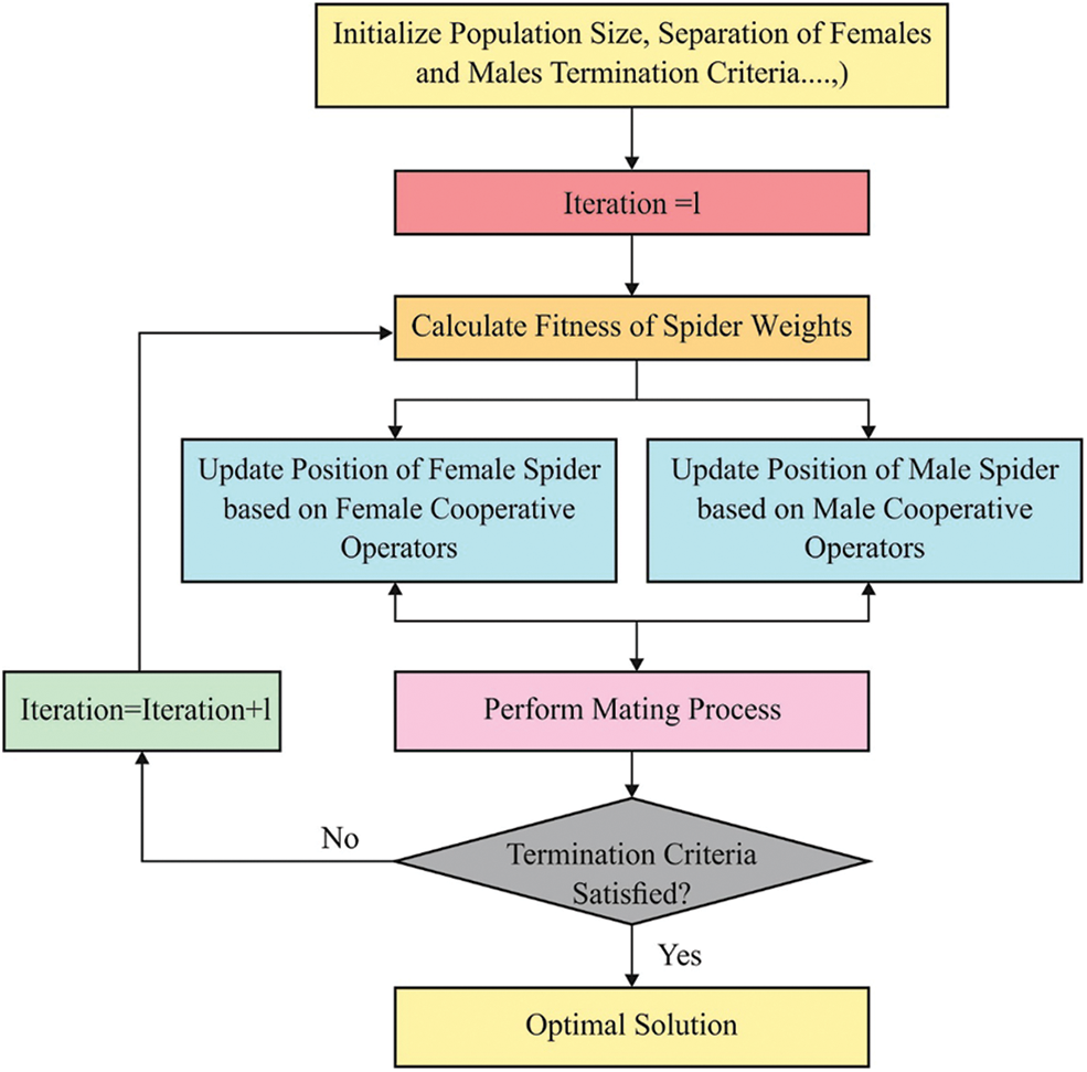
Figure 2: Flowchart of SSO technique

The mating phenomenon occurs when there is minimum of one efficient male (EM) and one female neighboring the effectual male in a cycle with predefined radius (PR). The mating function purposes for producing further spiders to drive population diversity and also purposes for replacing solutions with low quality. The middle of cycle is the place of leading male. Therefore, the spider inside the cycle is named a mating member. The PR has computed as the subsequent formula.

PR=∑j=1NV(xj,max−x)2⋅NCV(14)

All the mating members are allocated a value of effect probability IPs with utilizing roulette selective approach. The IPs is defined as the subsequent formula:

IPs=ws∑s=1Nmatews(15)

Thus the outcome, novel spiders are created by the mating function. But, not all novel spiders are adapted and permitted that member of existing populations. It is capable that inserted as to existing populations in case their weight was superior to the worse spider. Conversely, the inserted spider is allocated by similar gender to worse spider. Now, the worse spider was rejected and it stops being a member of the population.

4  Experimental Validation

In this section, the performance validation of SSODLSA-SGS algorithm takes place using a dataset which comprises of two classes namely stable and unstable [19]. The actual number of instances in the unstable and stable classes are 6380 and 3620 respectively. After SMOTE process, the number of instances in the unstable and stable classes becomes 6380 and 6350 respectively.

Fig. 3 depicts the correlation matrix analysis of SSODLSA-SGS technique under distinct attributes.

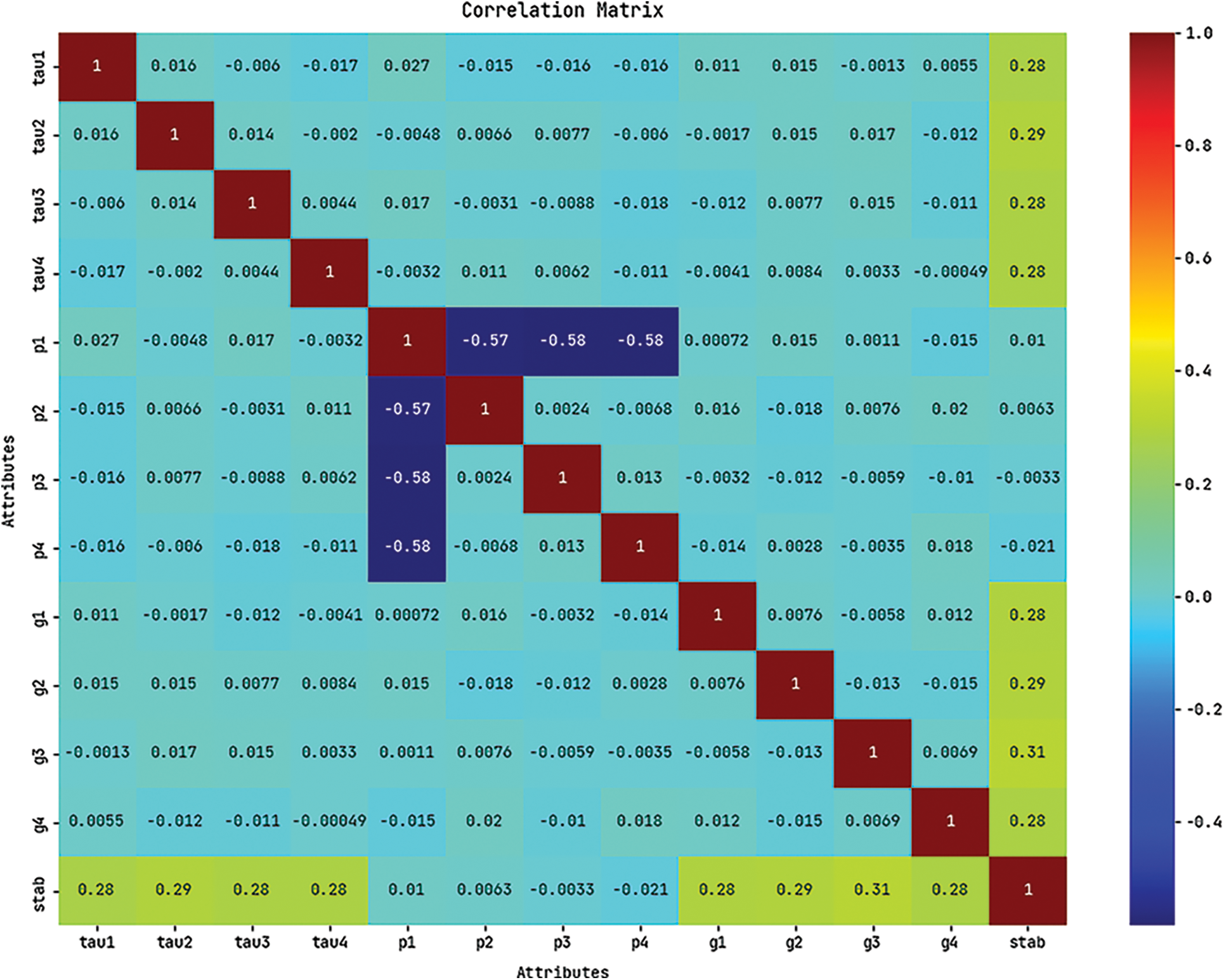
Figure 3: Correlation matrix of SSODLSA-SGS technique

Fig. 4 shows the pairwise relationship plot of the class labels involved in the test dataset.

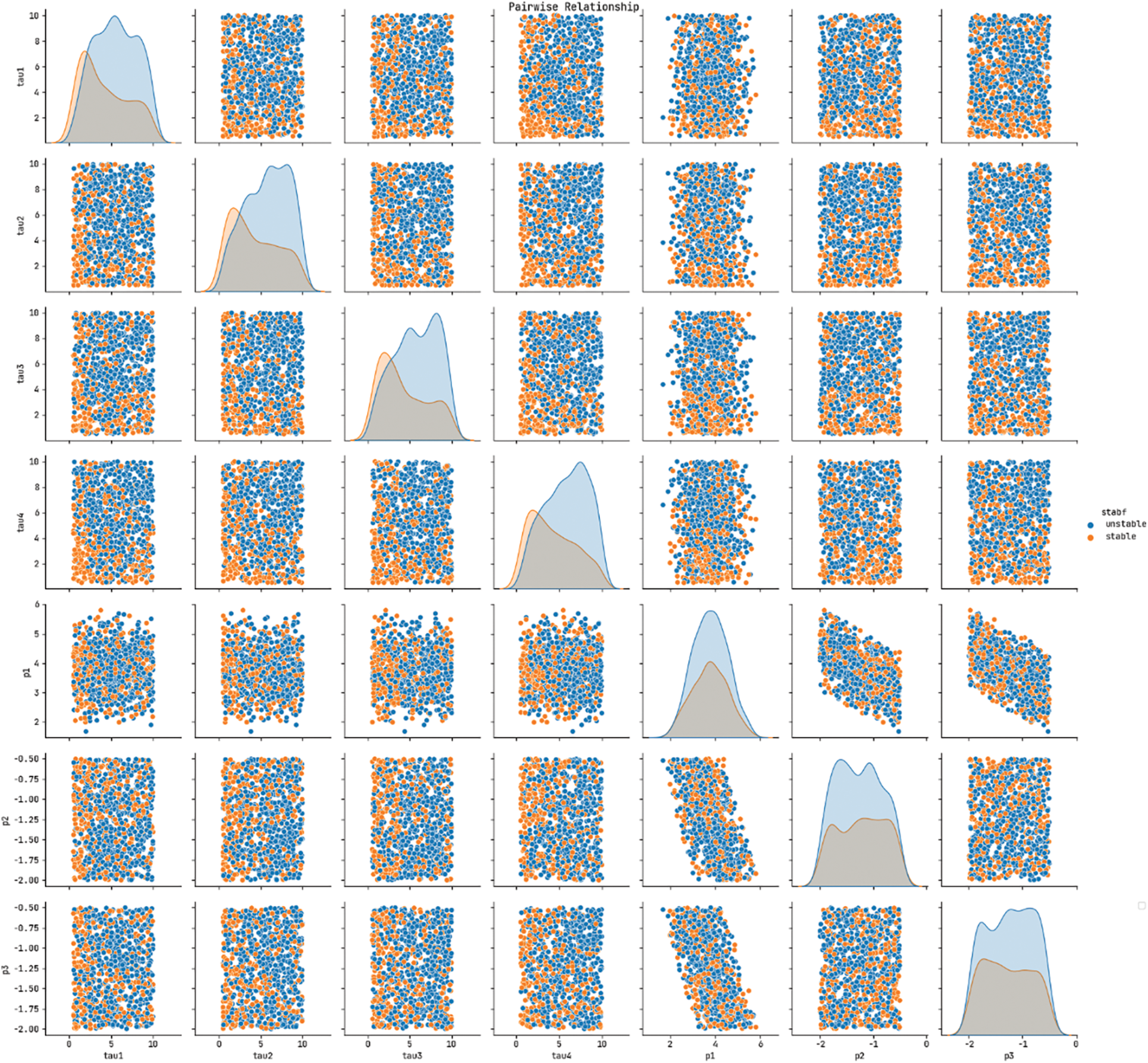
Figure 4: Pairwise relationship of class labels

Fig. 5 exhibits the set of five confusion matrices produced by the SSODLSA-SGS model under five distinct runs. The figures reported that the SSODLSA-SGS model has received effectual classification outcome under each run. For instance, on run-1, the SSODLSA-SGS model has identified 1904 samples under unstable class and 1904 instances under stable class. In addition, on run-3, the SSODLSA-SGS model has recognized 1909 samples under unstable class and 1901 instances under stable class. Also, on run-5, the SSODLSA-SGS model has recognized 1904 samples under unstable class and 1901 instances under stable class.

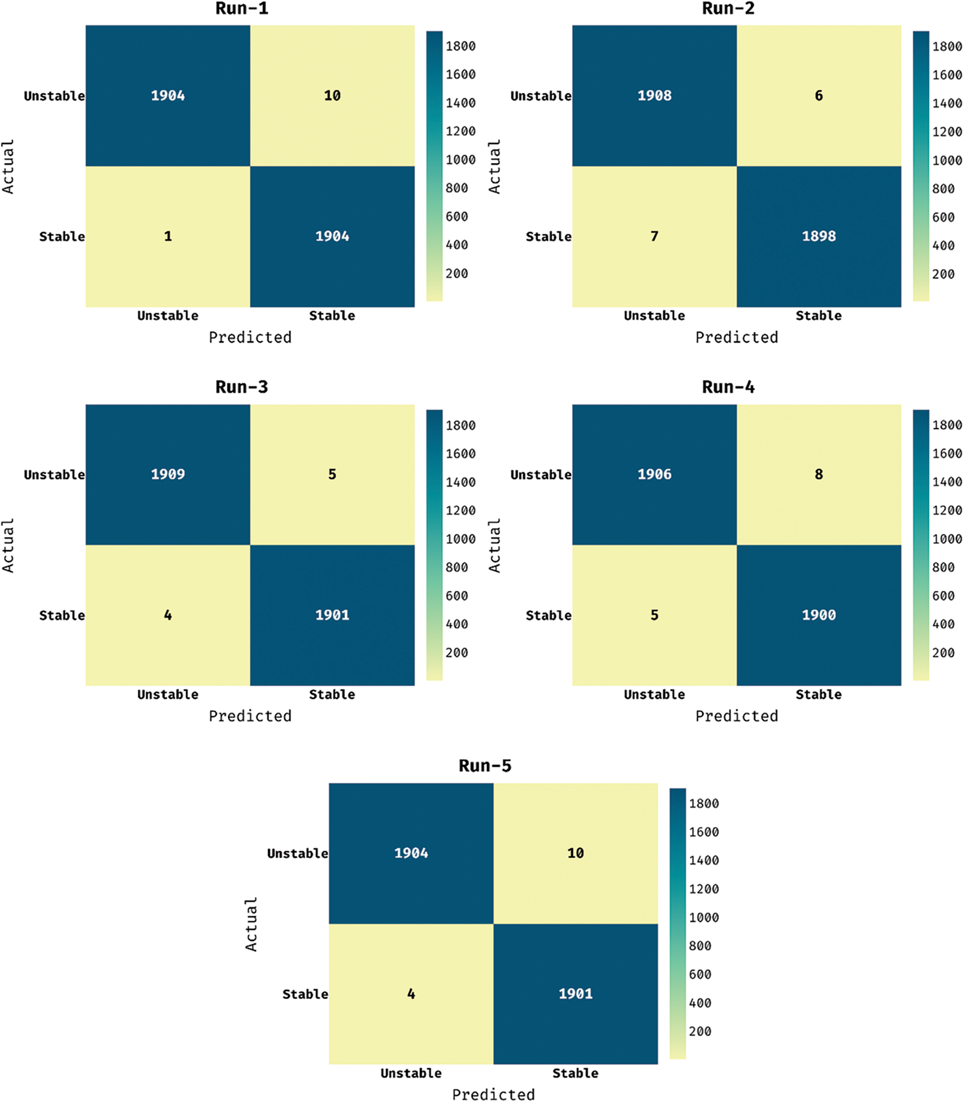
Figure 5: Confusion matrix of SSODLSA-SGS technique under five runs

Tab. 1 reports the overall SG predictive results of the SSODLSA-SGS model on different runs of execution. Fig. 6 portrays the precn, recal, and accuy examination of the SSODLSA-SGS model under distinct runs. The results reported that the SSODLSA-SGS model has accomplished effectual values of precn, recal, and accuy. For instance, with run-1, the SSODLSA-SGS model has offered precn, recal, and accuy of 0.9995, 0.9948, and 0.9971 respectively. Moreover, with run-2, the SSODLSA-SGS model has provided precn, recal, and accuy of 0.9963, 0.9969, and 0.9966 respectively. In line with, with run-5, the SSODLSA-SGS model has resulted to precn, recal, and accuy of 0.9979, 0.9948, and 0.9963 respectively.

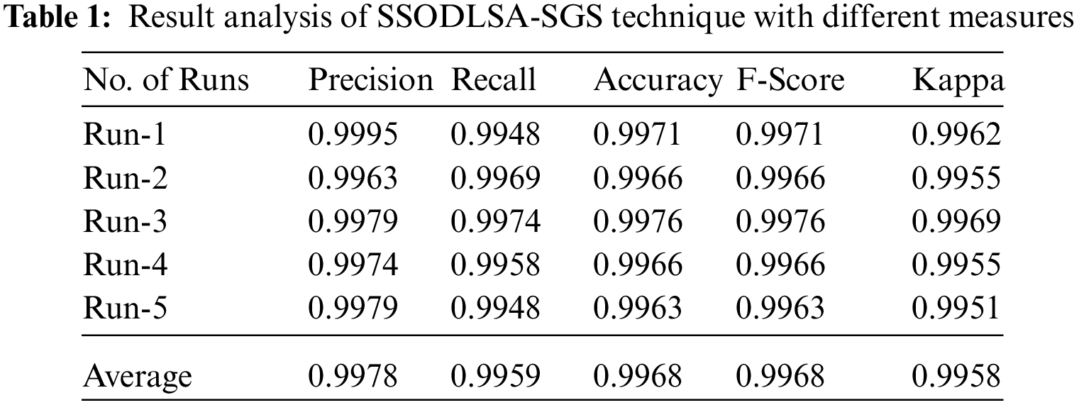
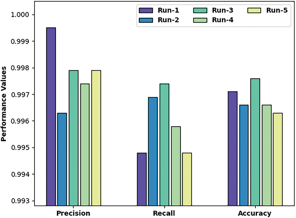
Figure 6: Result analysis of SSODLSA-SGS technique with distinct measures

Fig. 7 exhibits Fscore and kappa inspection of the SSODLSA-SGS model under dissimilar runs. The figure indicated that the SSODLSA-SGS model has accomplished enhanced values of Fscore and kappa. For example, with run-1, the SSODLSA-SGS model has exhibited Fscore and kappa of 0.9971 and 0.9962 respectively. Besides, with run-2, the SSODLSA-SGS model has depicted Fscore and kappa of 0.9966 and 0.9955 respectively. Furthermore, with run-5, the SSODLSA-SGS model has demonstrated Fscore and kappa of 0.9963 and 0.9951 respectively.

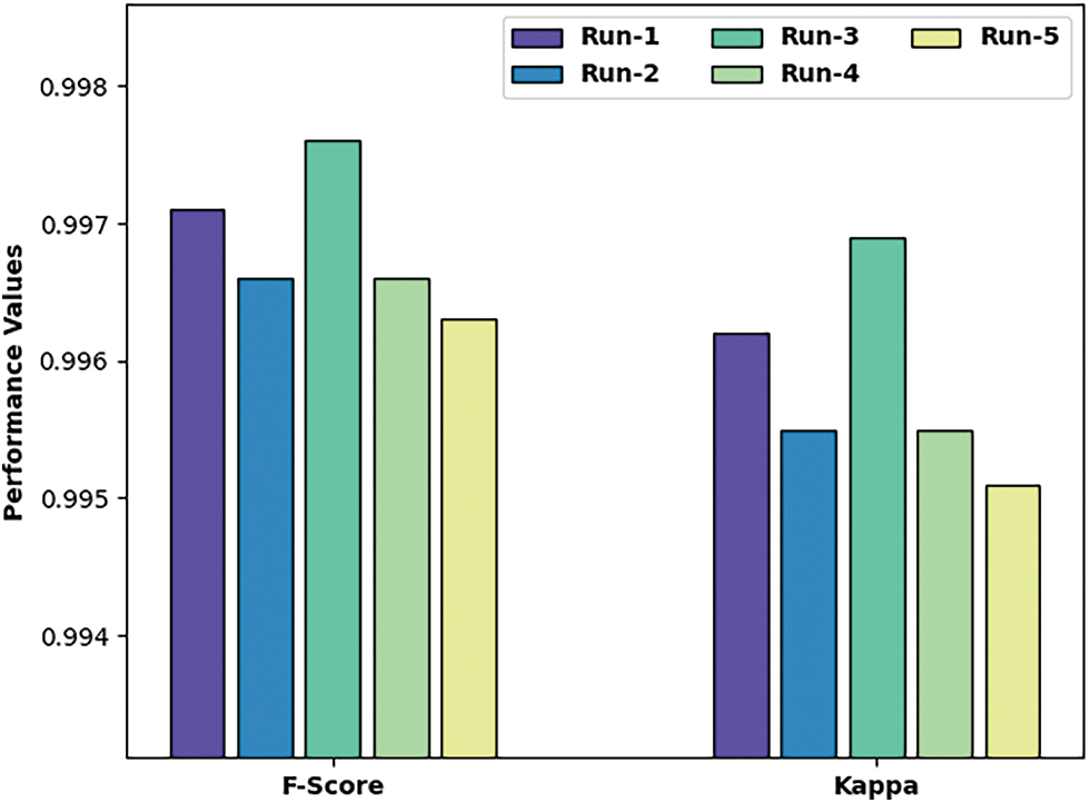
Figure 7: Fscore and kappa analysis of SSODLSA-SGS technique

Fig. 8 highlights the average SG stability result analysis of the SSODLSA-SGS model on the test dataset. The figure reported that the SSODLSA-SGS model has shown effective SG stability prediction performance with the increased average precn of 0.9978, recal of 0.9959, accuy of 0.9968, Fscore of 0.9968, and kappa of 0.9958.

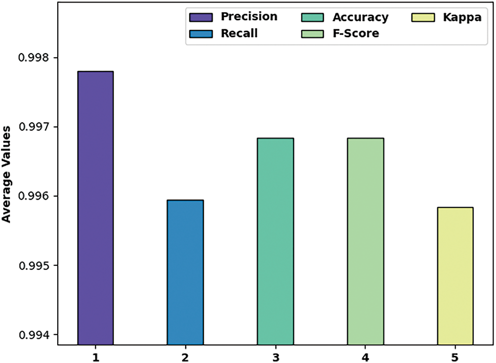
Figure 8: Average analysis of SSODLSA-SGS technique with various measures

The accuracy outcome analysis of the SSODLSA-SGS technique under run-3 is portrayed in Fig. 9. The outcomes demonstrated that the IHPT-DLMD approach has accomplished higher validation accuracy compared to training accuracy. It is also observable that the accuracy values get saturated with the count of epochs.

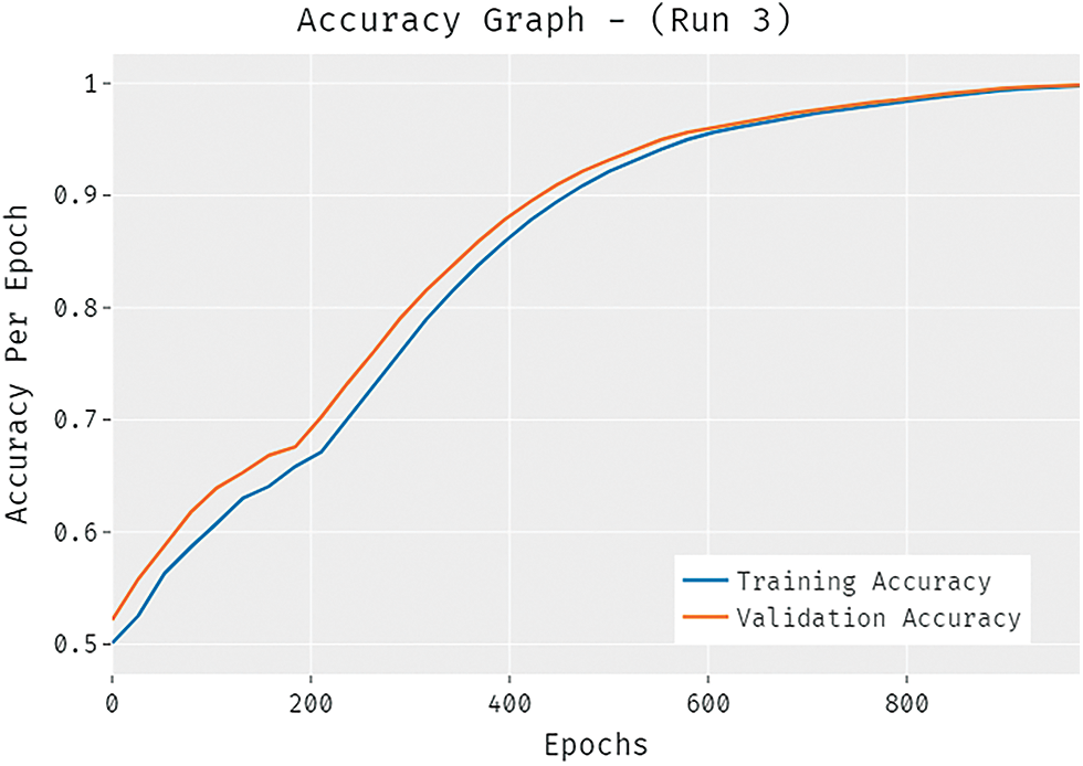
Figure 9: Accuracy analysis of SSODLSA-SGS technique under run-3

The loss outcome analysis of the SSODLSA-SGS system under run-3 is showed in Fig. 10. The figure exposed that the IHPT-DLMD algorithm has denoted the reduced validation loss over the training loss. It can be additionally noticed that the loss values get saturated with the count of epochs.

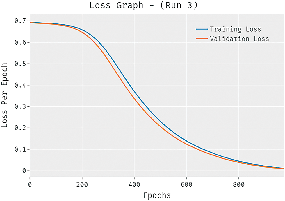
Figure 10: Loss analysis of SSODLSA-SGS technique under run-3

For demonstrating the promising performance of the SSODLSA-SGS model, a comparative accuy analysis is performed in Tab. 2 and Fig. 11. The result indicated that the CAR model has accomplished least accuy of 0.8000. At the same time, the BR, DT, and CNN models have resulted to certainly improved accuy values of 0.9160, 0.9030, and 0.8922 respectively.

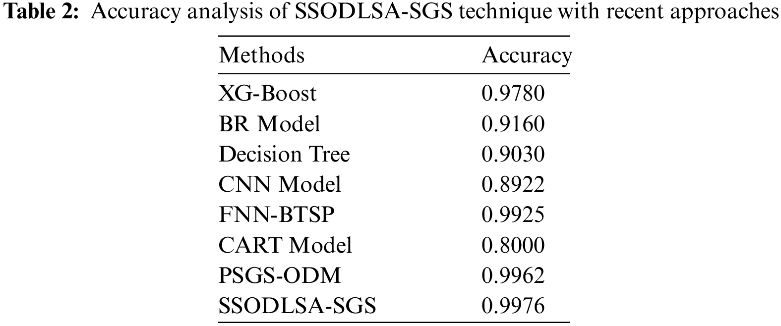
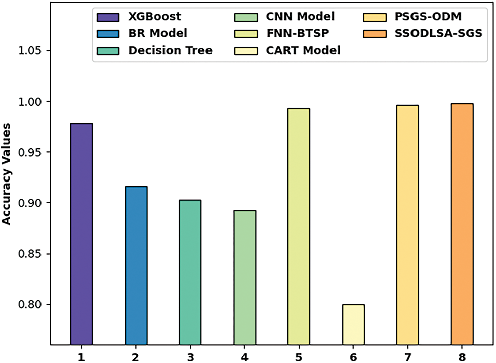
Figure 11: Accuy analysis of SSODLSA-SGS technique with recent approaches

Along with that, the XGBoost, FNN-BTSP, and PSGS-ODM techniques have reached reasonable accuy values of 0.9780, 0.9925, and 0.9962 respectively. However, the SSODLSA-SGS model has resulted in superior accuy values of 0.9976. From the detailed results and discussion, it is ensured that the SSODLSA-SGS model has resulted in higher predictive outcome over the other models.

5  Conclusion

In the study, a SSODLSA-SGS technique has been developed is to determine the stability level in the SGs. The proposed SSODLSA-SGS technique comprises data pre-processing (data normalization and transformation), DBN-BN based prediction, and SSO based hyperparameter optimization. The design of SSO algorithm helps to appropriately modify the hyperparameter values of the DBN-BN model. A series of simulation analyses are conducted to highlight the enhanced outcomes of the SSODLSA-SGS model. The extensive comparative study reported the improved efficiency of the SSODLSA-SGS algorithm over the other recent techniques interms of several measures. In future, data clustering and feature selection models can be included to improve the predictive outcomes.

Funding Statement: The authors received no specific funding for this study.

Conflicts of Interest: The authors declare that they have no conflicts of interest to report regarding the present study.

References

1. O. Omitaomu and H. Niu, “Artificial intelligence techniques in smart grid: A survey,” Smart Cities, vol. 4, no. 2, pp. 548–568, 2021. [Google Scholar]

2. S. Li, J. Hou, A. Yang and J. Li, “DNN-based distributed voltage stability online monitoring method for large-scale power grids,” Frontiers in Energy Research, vol. 9, pp. 625914, 2021. [Google Scholar]

3. A. B. Risco, R. I. G. Salinas, A. O. Guerrero and D. L. B. Esparta, “IoT-based SCADA system for smart grid stability monitoring using machine learning algorithms,” in 2021 IEEE XXVIII Int. Conf. on Electronics, Electrical Engineering and Computing (INTERCON), Lima, Peru, pp. 1–4, 2021. [Google Scholar]

4. W. Sun, G. Z. Dai, X. R. Zhang, X. Z. He and X. Chen, “TBE-Net: A three-branch embedding network with part-aware ability and feature complementary learning for vehicle re-identification,” IEEE Transactions on Intelligent Transportation Systems, pp. 1–13, 2021. https://doi.org/10.1109/TITS.2021.3130403 [Google Scholar] [CrossRef]

5. W. Sun, L. Dai, X. R. Zhang, P. S. Chang and X. Z. He, “RSOD: Real-time small object detection algorithm in UAV-based traffic monitoring,” Applied Intelligence, vol. 92, no. 6, pp. 1–16, 2021. [Google Scholar]

6. M. A. Mahmoud, N. R. M. Nasir, M. Gurunathan, P. Raj and S. A. Mostafa, “The current state of the art in research on predictive maintenance in smart grid distribution network: Fault’s types, causes, and prediction methods—A systematic review,” Energies, vol. 14, no. 16, pp. 5078, 2021. [Google Scholar]

7. Y. Zhang, H. Zhang, J. Zhang, L. Li and Z. Zheng, “Power grid stability prediction model based on BiLSTM with attention,” in 2021 Int. Symp. on Electrical, Electronics and Information Engineering, Seoul Republic of Korea, pp. 344–349, 2021. [Google Scholar]

8. M. Xia, H. Shao, X. Ma and C. W. de Silva, “A stacked GRU-RNN-based approach for predicting renewable energy and electricity load for smart grid operation,” IEEE Transactions on Industrial Informatics, vol. 17, no. 10, pp. 7050–7059, 2021. [Google Scholar]

9. H. Yang, J. Zhang, J. Qiu, S. Zhang, M. Lai et al., “A practical pricing approach to smart grid demand response based on load classification,” IEEE Transactions on Smart Grid, vol. 9, no. 1, pp. 179–190, 2018. [Google Scholar]

10. M. A. A. Sufyan, M. Zuhaib and M. Rihan, “An investigation on the application and challenges for wide area monitoring and control in smart grid,” Bulletin of Electrical Engineering and Informatics, vol. 10, no. 2, pp. 580–587, 2021. [Google Scholar]

11. A. K. Bashir, S. Khan, B. Prabadevi, N. Deepa, W. S. Alnumay et al., “Comparative analysis of machine learning algorithms for prediction of smart grid stability†,” International Transactions on Electrical Energy Systems, vol. 31, no. 9, pp. 1–23, 2021. [Google Scholar]

12. M. Alazab, S. Khan, S. S. R. Krishnan, Q. V. Pham, M. P. K. Reddy et al., “A multidirectional LSTM model for predicting the stability of a smart grid,” IEEE Access, vol. 8, pp. 85454–85463, 2020. [Google Scholar]

13. M. Massaoudi, H. A. Rub, S. S. Refaat, I. Chihi and F. S. Oueslati, “Accurate smart-grid stability forecasting based on deep learning: Point and interval estimation method,” in 2021 IEEE Kansas Power and Energy Conf. (KPEC), Manhattan, KS, USA, pp. 1–6, 2021. [Google Scholar]

14. P. Breviglieri, T. Erdem and S. Eken, “Predicting smart grid stability with optimized deep models,” SN Computer Science, vol. 2, no. 2, pp. 73, 2021. [Google Scholar]

15. F. Rodríguez, A. Galarza, J. C. Vasquez and J. M. Guerrero, “Using deep learning and meteorological parameters to forecast the photovoltaic generators intra-hour output power interval for smart grid control,” Energy, vol. 239, pp. 122116, 2022. [Google Scholar]

16. N. V. Chawla, K. W. Bowyer, L. O. Hall and W. P. Kegelmeyer, “SMOTE: Synthetic minority over-sampling technique,” Journal of Artificial Intelligence Research, vol. 16, pp. 321–357, 2002. [Google Scholar]

17. J. Tian, Y. Liu, W. Zheng and L. Yin, “Smog prediction based on the deep belief - BP neural network model (DBN-BP),” Urban Climate, vol. 41, no. 2, pp. 101078, 2022. [Google Scholar]

18. S. Almufti, “The novel social spider optimization algorithm: Overview, modifications, and applications,” Icontech International Journal, vol. 5, no. 2, pp. 32–51, 2021. [Google Scholar]

19. https://github.com/pcbreviglieri/data-science-smart-grid-stability [Google Scholar]