MEB-YOLO: An Efficient Vehicle Detection Method in Complex Traffic Road Scenes

1  Introduction

One of the core roles of Computer Vision (CV) is object detection. Its major job is to find and classify items while identifying the region of interest in object pictures. Vehicle target detection is a popular study topic with significant research value and is quite difficult, which has drawn a lot of interest from academics [1–4].

The growth of the economy has increased the number of vehicles, which has caused several traffic issues, including heavy traffic and frequent accidents. Approaches like intelligent transportation systems [5], autonomous driving [6], and problematic vehicle tracking [7] have arisen to address these issues. Technology for vehicle detection is essential in these fields. The system for processing traffic accidents, managing traffic, vehicle transportation system, and managing public transportation are all included in the intelligent traffic system. It is mostly utilized in situations like toll collection at highway intersections, road order command, and vehicle control in and out of neighborhoods, all of which significantly lessen the workload of traffic management employees. Today’s approach to intelligent transportation systems relies on CV technology [8], which uses cameras to collect data on live traffic and relies on vehicle detection technology for road vehicle statistics. The advancement of vehicle detection technology is essential for autonomous driving since it allows for the precise recognition of moving vehicles on the road. Vehicle cameras pick up the car in front and relay that information back to the driverless system to ensure that the car drives smoothly. Currently, tracking problem vehicles is typically done by human resources, which is time-consuming and labor-intensive. Vehicle detection can help change the status quo to some extent by first identifying the type of vehicle the target belongs to, then choose the vehicle that most closely matches the target characteristics using computer technology, thereby realizing the tracking of the vehicle.

A prevalent research area is the application of deep learning-based target identification algorithms in the field of vehicle detection. To recognize automobiles without the issues associated with manually built features in traditional detection, Fan et al. [9] developed a Faster Region-based Convolutional Neural Network (Faster R-CNN). To enhance the Intersection over Union (IoU) threshold of candidate frames layer by layer and increase the detection accuracy of small objects, Cai et al. [10] presented the Cascade Regions with CNN Features (Cascade RCNN) network using a Cascade detector. To recognize road cars in real-time, Cheng et al. [11] transformed Darknet53 into a convolutional neural network with 30 convolutional layers and utilized K-means clustering to get vehicle anchor frames. To achieve real-time identification and enhance robustness against light changes, Abdelwahab et al. [12] suggested an effective automatic classification method based on compact image representations and deep residual networks. A vehicle detection model based on YOLOv3 was proposed by Ding et al. [13]. It uses four feature maps with various scales to extract more specific information and adds a residual structure to recover underlying vehicle features. To increase the generalizability of vehicle detection, Doan et al. [14] suggested an adaptive approach combining YOLOv4 with Deep Simple Online and Realtime Tracking (DeepSORT). Xu et al. [15] improved YOLOv3 by increasing the depth of networks and invoking the top-level feature maps to solve the problem of information loss. The CNN-based classifier and YOLO were integrated by Azimjonov et al. [16] to meet the demands of precise, lightweight, and immediate vehicle target detection. To increase the detection precision of tiny vehicle targets, Carrasco et al. [17] suggested a modified model based on YOLOv5 architecture. A Channel-Spatial Attention Fused Feature Pyramid Network (CSF-FPN) was created by Hou et al. [18] and effectively reduces the false detection rate and the missed detection rate when there is a significant volume of data. Xu et al. [19] proposed a model based on Shadow-Background-Noise 3D Spatial Decomposition (SBN-3D-SD), to accomplish 3-D spatial three-decomposition, it takes advantage of the sparse property of shadows, the low-rank property of backgrounds, and the Gaussian property of noises. By using the Alternating Direction Method of Multipliers (ADMM), it separates shadows from backgrounds and noises. Vehicle detection research still faces many difficulties [20], primarily due to the following factors: (1) The number of large-size vehicles in the existing vehicle data set is significantly higher than the number of small-size vehicles, and since the majority of the data set collection is carried out via high-speed or highway monitoring, the background of most of the collected pictures is fixed, making the background information in the data set insufficient. (2) The surface characteristics of vehicles will change with light and weather conditions, resulting in significant differences in the external characteristics of the same category of the vehicle; the appearance of various categories of vehicles of the same brand may be similar, resulting in minimal differences between various categories of vehicles; the limited visibility and varying camera angles of surveillance cameras will cause relatively significant changes in the size and stance of the same vehicle, making identification more challenging; the size of the background in the current dataset is far bigger than the area occupied by the target car in the image, making it difficult to extract the information needed to identify the target vehicle’s features. It is necessary to accurately extract the features of the vehicle in the image in the early stage to solve the issues brought on by these various scenarios. The ability to exist detection models to extract features still has a lot of space for development. (3) The likelihood of false detection and missed detection is significantly increased in situations where the road is crowded, the vehicle target is small, or the vehicle is hidden by other objects. (4) The existing target detection algorithms’ detection speeds are still insufficient for the real-time, precise detection of cars under challenging traffic circumstances. Additionally, the target detection model has too many layers, model training takes too long, the computational cost is too high, and the target detection equipment’s high processing power is needed.

This work proposes the MEB-YOLO, a novel vehicle detection classification approach, to address these issues. Our main contributions are summarized as follows:

(1) The Mosaic and MixUp data enhancement technologies are used during the dataset processing stage. The dataset’s background information can be improved, and the number of small targets can be raised.

(2) It employs a brand-new feature extraction network. The CSPDarknet network now uses the ECA attention mechanism and the Activate or Not (ACON) activation function. ECA can enhance the feature expression strength of each channel without adding too many parameters, which enhances the feature extraction ability of the backbone network, which enhances the detection accuracy of the vehicle detection model. ACON helps to improve the generalization ability of the model and the information transfer efficiency of each feature layer while reducing the computation and complexity of the model.

(3) The usage of the BiFPN structure improves feature integration, expands the use of multi-scale target feature data in the high-level feature maps, and yields more high-level feature fusion without raising the computational costs. With a smaller model size and lower computational cost, this structure can also outperform earlier detection methods in terms of efficiency and accuracy.

(4) Decoupled Head, Anchor Free approach, and Simplified Optimal Transport Assignment (SimOTA) are employed to get the final prediction results. The use of Decoupled Head structure effectively accelerates the model convergence speed and improves the model accuracy; the use of Anchor Free approach reduces the computational volume, decreases the computational cost, and resolves the positive and negative sample imbalance problem; the use of the SimOTA algorithm significantly enhances the multi-objective coupling problem common in open scenes, cuts down on training time, and increases vehicle detection accuracy.

The rest of the paper is structured as follows. Section 2 examines the relevant literature. The suggested MEB-YOLO vehicle detection model’s framework is described in depth in Section 3. The dataset used in the experiments, different model parameters, the environment configuration, as well as the pertinent evaluation metrics employed in the experiments, are all introduced in Section 4. Section 5 compares the experimental results of the MEB-YOLO with cutting-edge vehicle detection models. In Section 6, conclusions are attained.

2  Related Work

Traditional road target detection algorithms and deep learning-based road target detection algorithms are two categories of widely used road target detection techniques. Deep learning-based road target detection algorithms are now widely used.

There are three phases in the conventional target detection method. First, prospective regions in the image where objects are expected to occur are found using the selective search algorithm [21]. After obtaining the candidate regions, a variety of extractors can be used to extract pertinent visual features. For example, the harr [22] algorithm is frequently used to detect faces, the Histogram of Oriented Gradient (HOG) [23] algorithm is frequently used to find pedestrians, and the Scale-Invariant Feature Transform (SIFT) algorithm [24] is frequently used to extract local features. Support Vector Machine (SVM) classifier [25] and other popular classifiers are used to categorize the target item at the end. Traditional detection techniques are slow and inaccurate, and they perform poorly in some traffic photographs with complicated backdrops.

Deep learning-based road target detection algorithms have increasingly gained popularity as computer performance has increased and have produced outstanding outcomes in the sectors of text recognition, speech recognition, and computer vision [26–28]. Road target identification methods based on deep learning combine low-level characteristics to create high-level features, enhancing the model’s capacity to detect targets. Deep learning-based methods outperform conventional road target identification algorithms for numerous classification tasks of road targets in terms of stability, robustness, and computational speed. Deep learning-based road target detection systems come in two primary categories. Region-based Convolutional Neural Networks (R-CNN) [29] and Faster R-CNN [30], for example, are two-stage road target detection algorithms based on target candidate frames. The other is one-stage end-to-end model-based road target identification techniques, such as YOLO [31], Single Shot Multi-Box Detector (SSD) [32], YOLOv2 [33], YOLOv3 [34,35], etc.

A selective search method is used in the first stage of the two-stage target detection algorithm to identify the target candidate regions. Convolutional Neural Network (CNN) classifier is then used to determine the category and to perform detection frame regression. The LeNet system was proposed by Lecun et al. [36] in 1998 and is mostly used for handwritten character recognition. A flurry of CNN applications in the field of computer vision was sparked in 2012 when Krizhevsky et al. [37] employed AlexNet to generate positive outcomes on the ImageNet dataset. R-CNN target detection system was proposed by Girshick et al. [29] in 2014, integrating support vector machines and BP (backpropagation) trained CNN as classifiers. The Spatial Pyramid Pooling Network (SPPNet) was proposed by He et al. [38], which overcomes the requirement that the input photos must be of the same size. Ren et al. [30] proposed an improved end-to-end detection method called Faster-R-CNN based on the principle of R-CNN, which may shorten training time and increase detection effectiveness. Models with two stages can attain better detection precision, however, they fall short of the real-time requirement.

One-stage detection techniques omit the candidate box extraction step and implement feature extraction, candidate box classification, and regression directly in a deep convolutional network. The SSD technique was proposed by Liu et al. [32] and uses a feature pyramidal hierarchy to identify regression. In 2016, Koirala et al. [31] proposed YOLO, which exclusively employs convolutional computing to do real-time feature extraction, classification, and regression on prediction boxes. It is the first one-stage, real-time object detection model to treat detection as a regression task. Sang et al. [33] proposed YOLOv2 in 2017 to increase the detection speed and localization accuracy of YOLO. The feature pyramid network was introduced in 2018 by Redmon et al. [34], who offered the YOLOv3 method to lower the rate of missed identification of small targets. The YOLOv4 model, which Bochkovskiy et al. [39] presented, offers an effective and potent object detection model that perfectly detects small objects. In 2018, Law et al. [40] developed the Corner Network (CornerNet), which produced heat maps and embedding vectors using a single convolutional model. A small-scale, high-precision, and more effective object detection network called EfficientDet was proposed by Tan et al. [41] in 2020. It leverages EfficientNet as its backbone network for effective bidirectional cross-scale connectivity and weighted feature fusion [42]. Liu et al. [43] proposed the Swin Transformer, which is a Transformer-based backend for computer vision tasks, and the authors have shown through extensive experiments that the shift window requires only a small overhead to increase the detection accuracy. Long et al. [44] proposed the most advanced target detection model at the time named PP-YOLO. This model was applied to the UA-DETRAC dataset for vehicle detection, and it produced reasonably successful results. Due to its benefits of high accuracy, speed, and scalability, YOLOv5 [45] has emerged as one of the most used models for target recognition. A brand-new, high-performance detector called YOLOX that is not restricted by prior bounding boxes was proposed by Ge et al. [46]. YOLOX can detect target regions at various scales more effectively than other one-stage algorithms. Xu et al. [47] proposed a lightweight on-board SAR ship detector called Lite-YOLOv5, it is frequently utilized in the field of marine surveillance because Lite-YOLOv5 can quickly and accurately recognize ship pictures in microwave remote sensing images produced by Synthetic Aperture Radar (SAR). Wang et al. [48] proposed YOLOv7, which outperforms all known target detection algorithms in the range of 5FPS~160FPS in terms of speed and accuracy, and is optimized for both model architecture and training process. The Deep Automated Machine Learning combined YOLO (DAMO-YOLO) proposed by Xu et al. [49] introduces several new techniques based on the YOLO framework and significantly modifies the entire detection framework. With a new detection backbone structure based on Neural Architecture Methods (NAS) search, a deeper neck structure, a streamlined head structure, and the introduction of distillation techniques to further improve the results. To quickly address real-world issues in industrial implementation, DAMO-YOLO also offers efficient training strategies and simple deployment tools.

Target detection is now a field in which saliency detection [50,51] has a wide range of applications. To find the most “salient” portions in an image, saliency detection employs image processing methods and computer vision algorithms. The “salient” portions are those parts of the image that stand out or are significant, such as the parts that the human eye will gravitate toward first while examining an image. Saliency detection is the process of automatically identifying key regions of an image or a scene. The algorithm can only identify portions of the image where it “thinks” there is a target, which may or may not include a target. Saliency detection is not target detection, and it does not determine whether there is a “target” in the image. Algorithms for saliency detection can be used to detect salient regions as the initial stage in a target detection task, after which these regions will be the subject of assessments and predictions. Saliency detections are often extremely quick algorithms that can function in real-time. The results of the saliency detection are subsequently passed to the more computationally intensive algorithm. This way the subsequent computationally intensive algorithm does not have to run on every region of the image, but only on the salient region.

3  The Proposed Method

This section elaborates on the basic operation of the proposed single stage vehicle detection model. To identify and classify vehicles in photographs of road vehicles, a new MEB-YOLO technique is devised. Fig. 1 depicts the proposed model’s overall structure. The MEB-YOLO model has several steps for locating and detecting vehicles. The dataset is firstly pre-processed by MixUp and Mosaic data augmentation before model learning. The improved CSPDarknet then uses the processed dataset to extract useful features. BiFPN then does feature fusion to combine feature data from various scales. To get detection frames that comprise the position information as well as the category information of the target objects, the Prediction module is utilized to classify and regress the feature information. The overall process of the vehicle detection model is shown in Algorithm 1.

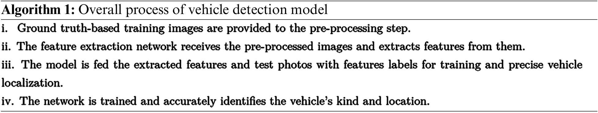
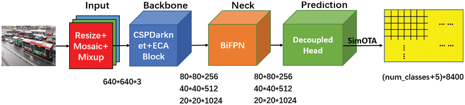
Figure 1: The structure of the proposed MEB-YOLO model

3.1 Image Pre-processing

The amount of large-size targets in the datasets currently being used for target detection training is significantly higher than the number of small-size targets and also has the drawback that the images do not contain enough background data. Pre-processing the dataset is therefore something we should do to improve this issue. The Mosaic data augmentation stitches together four separate photos to create a single image, and then trains them to accomplish the effect of indirectly raising the batch size. The MixUp data augmentation approach can combine two photographs with various object classes in a specific ratio to create a new image, which has the effect of increasing the training dataset. Examples of MixUp and Mosaic are shown in Figs. 2 and 3, respectively. Pre-processing the dataset can improve the image backgrounds, increase the number of tiny target objects, and strengthen the network. This approach can reduce the false rate and missing rate of the model.

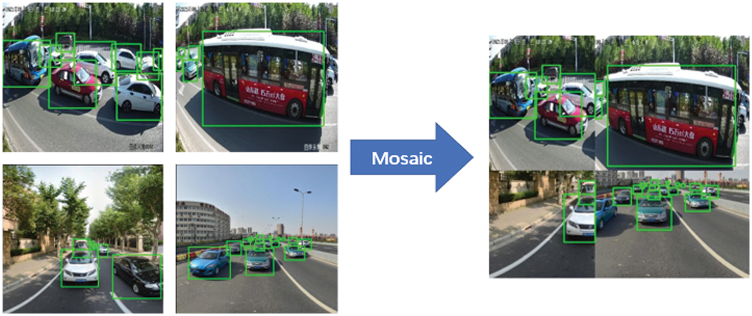
Figure 2: Example of Mosaic

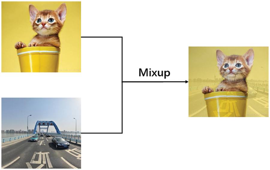
Figure 3: Example of MixUp

3.2 Backbone: Feature Extraction

Feature extraction of an image is necessary for the computer to analyze the data and information included in the image. CNN is typically used by the target detection model to extract features. The feature map gets smaller as network layers are added, while the receptive field of pixel dots is bigger and the semantic information of features gets stronger. Smaller feature maps have the effect of making the information about small items difficult to extract or even disappear, which negatively affects the model’s ability to detect small things.

The CSPDarknet can gather rich semantic information about small objects by the continuous downsampling of image feature layers through convolution processes. The improved Cross Stage Partial Residual Network (CSPResNet) network’s general layout and filter parameters are followed by the CSPDarkNet network. The distinction is that each residential block is given a Cross Stage Partial (CSP) structure via CSPDarkNet. We’ve used a variety of enhanced techniques based on CSPDarkNet, employing a new structure as the feature extraction network, to assist the network in learning more expressive features, decrease the number of parameters, and better realize real-time detection. Five key features of CSPDarknet include:

1.    The residual network makes up the entirety of the backbone network portion. When there are too many layers in a deep neural network, gradient disappearance becomes a problem. The residual network uses a jump structure to address this issue. Increasing the depth of the residual network will increase the detection model’s accuracy.

2.    The Cross Stage Partial Network (CSPNet) structure is implemented, which divides the initial residual network structure into two parts. One of these portions continues the initial residual block stacking, and the other is connected directly to the endpoint after a few processing steps. CSPNet and deep Residual Networks (ResNet) combined can increase CNN’s capacity for learning, minimize computation, and increase internal storage.

3.    It makes advantage of the Focus network architecture. Four distinct feature layers are obtained by collecting values for each skipped pixel of an image. The channel information is amplified by four by stacking these feature layers.

4.    The Sigmoid Linear Unit (SiLU) activation function is used, which can be regarded as a smooth Rectified Linear Unit (ReLU) activation function, but it outperforms ReLU in-depth models. SiLU is nonmonotonic, smooth, and has a lower bound without an upper bound. The equation of SiLU is shown in Eq. (1):

SiLU(x)=x∗sigmoid(x)(1)

The equation of sigmoid is shown in Eq. (2):

sigmoid(x)=11+e−x(2)

5.   It makes use of the SSP structure, which was first employed in YOLOv4’s feature fusion phase. In our model, the backbone network makes advantage of it. The network’s perceptual field can be improved, and features can be efficiently extracted by employing pooling kernels of various sizes to execute the maximum pooling operation.

The following three issues are associated with the feature extraction process used by CSPDarknet. The complexity of operations will significantly grow as the number of convolution kernels increases. The global feature information will be lost if the receptive field is too small. Only a small portion of the local information in the original data can be recovered due to the global invariance of the convolution structure, which makes it insensitive to the global position information. Therefore, to improve the model, we implement the next two steps.

1.    The ACON activation function, which has superior qualities like non-saturation and sparsity and is used in replacement of the SiLU activation function, can occasionally have serious negative effects in the form of neuron necrosis. The degree of linearity of the activation function can be dynamically changed at various feature layers when using the ACON activation function. The model’s ability to generalize and transfer information is aided by this specially designed activation function for various feature layers, which also somewhat lessens the computing complexity of the model.

2.    A channel attention mechanism is added in the model, which can help the deep CNNs achieve better functionality and increase detection accuracy. The attention module can increase the expression strength of each channel’s features, sharpen the focus on the intended area, lessen the impact of background data, and increase the precision of small item recognition. Convolutional Block Attention Module (CBAM) [52], Squeeze and Excitation (SE) [53], and ECA [54] are the current common attention modules. We discovered through comparison testing that the ECA attention module can significantly enhance the performance of our model. ECANet suggested a local cross-channel interaction technique without dimensionality reduction and an adaptive selection of the one-dimensional convolutional kernel size to achieve performance improvements. According to Fig. 4, the ECA Block swaps out the fully linked layer for a one-dimensional convolution, whose kernel size is determined by the number of channels C. Without dimensionality reduction, channels are averaged globally. A one-dimensional convolution of size k is used to capture the information about the local cross-channel interactions between each channel and its k nearest neighbors. The number of nearby adjacent channels that are engaged in this channel’s attention prediction is represented by the convolution kernel size k, which also shows the coverage of local cross-channel interactions. To fully fuse the inter-channel interactions, k value size varies with the number of channels.

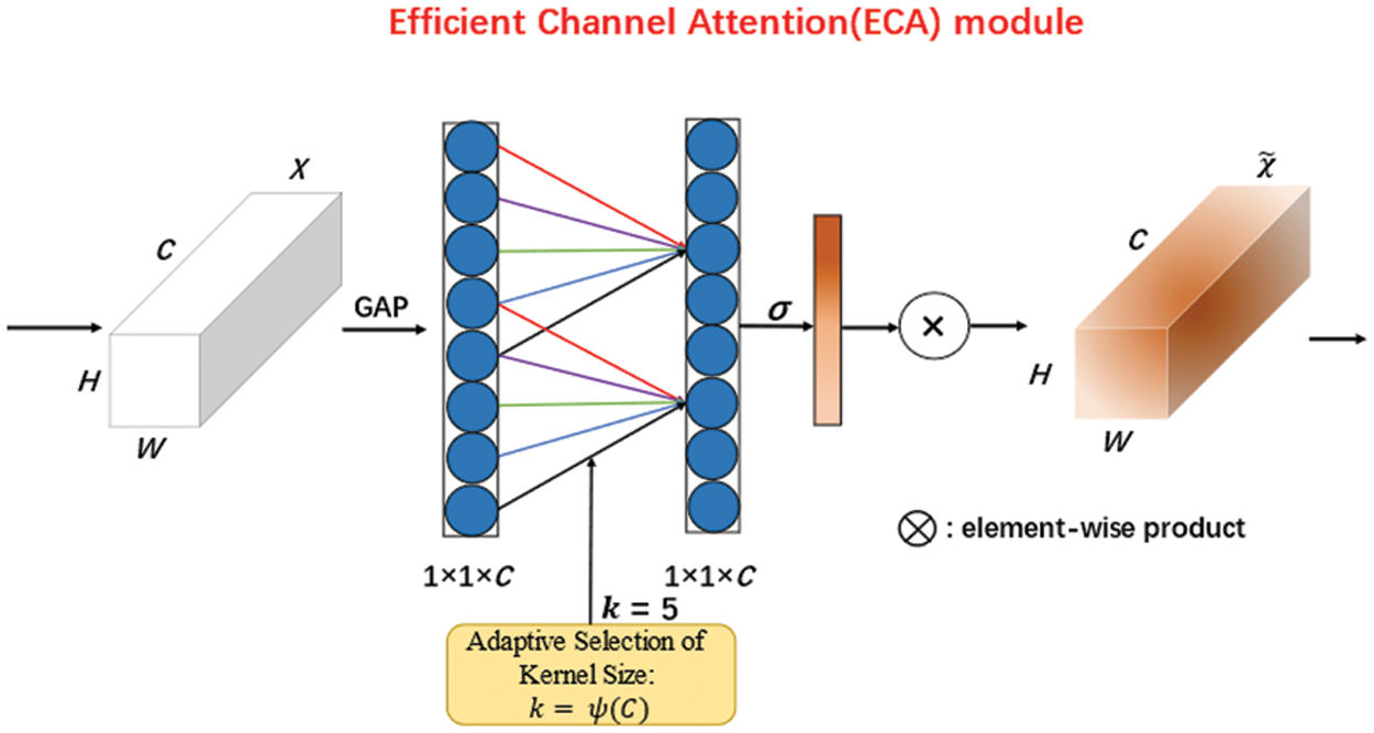
Figure 4: The structure of the ECA attention mechanism

Fig. 5 depicts the modified Backbone’s structural layout. First, ACON is used to replace the original activation function in CSPDarknet. The attention module is then added to CSPDarknet at the bottom. Fig. 6 depicts the precise structure of the CSP, SPP, Focus, and CBA modules in CSPDarknet.

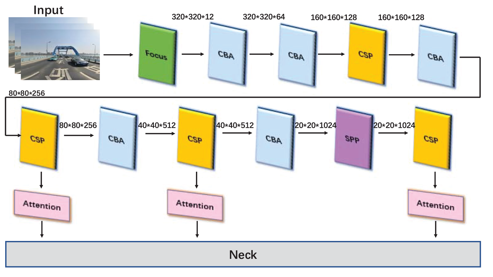
Figure 5: The structure of CSPDarknet

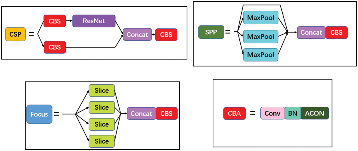
Figure 6: The details of each module in the backbone

3.3 Neck: BiFPN

The effectiveness of target detection is known to be directly influenced by the strength of the semantic information. To enhance the Neck network’s capacity to handle complex features, we must select an effective feature fusion network to handle the features extracted by the feature extraction network for each layer. The EfficientDet network model contains a structure called BiFPN, which is an effective structure for weighted feature fusion and bi-directional cross-scale connection. BiFPN was used in place of the original Neck network in the YOLOv4 model by Wang et al. [55], who discovered that SimOTA this dramatically enhanced the model’s detection speed and lowered the model’s parameters. Using this as a lesson, we discover an ideal means to include BiFPN as the model’s Neck network, and Fig. 7 depicts the BiFPN structure.

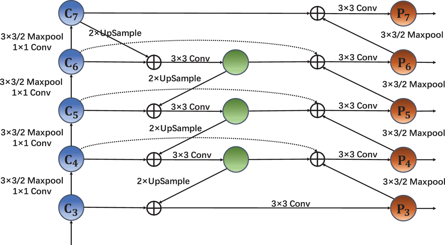
Figure 7: BiFPN feature pyramid network structure

The BiFPN network is an improvement based on Path Aggregation Network (PANet). To simplify the network, nodes with a single input are first deleted. The next step is to provide connections between input and output nodes at the same layer, which can integrate more practical features without incurring additional expenditures. Last but not least, each bidirectional path is repeated multiple times to create the effect of combining complex features.

The BiFPN structure uses a rapid normalized fusion operation to distribute different weights to input features of multiple resolutions to address the issue that the traditional feature fusion structure cannot discriminate the input features of different resolutions. This weighted fusion process is straightforward and efficient. The weighted fusion mechanism’s calculation formula is displayed in Eq. (3).

O=∑iwiϵ+∑jwj∗Ii(3)

where O stands for the output result, Ii(i=1,2,3,4,5) for the input at level i, wi for the learnable weighted input features at level I, and ϵ for a minimum value that approximates zero to prevent unstable computation outputs. The ultimate output values of each layer are displayed in Eq. (4) after BiFPN, and the weighted fusion technique have been combined.

Pnout=Conv(w1′⋅Pnin+w2′⋅Pntd+w3′⋅Resize(Pn−1inout)w1′+w2′+w3′+ϵ)(4)

where Pntd represents the features of the intermediate layers in the same layer, Resize usually represents down sampling or up sampling operations, Pnin represents the input feature at level n, Pninout denotes the output result at level n on bottom-up BiFPN pathways. We have developed the parameter weight wm′ (m = 1, 2, 3) to distinguish the relative relevance of various aspects in the feature fusion process, similar to the attention mechanism.

Similar to Softmax [56], this weighted fusion computation approach controls the outcomes in [0, 1]. BiFPN can finally accomplish fast normalized fusion and bi-directional cross-scale connectivity. The succeeding prediction network will use the five feature layers obtained from the feature extraction network to make predictions.

3.4 Prediction Module

Three enhanced feature layers are created after the feature fusion step using the BiFPN structure, and these feature layers are then input to the Prediction module to produce the detection results. Certain effective structures are required to increase the predictive power of the prediction module and allow the prediction network to accurately anticipate the position of the item, the probability that the detection frame contains the target object, and the class to which the object belongs. The Decoupled Head module, Anchor Free structure, and SimOTA are employed in our proposed strategy to increase the prediction module’s capacity.

The Decoupled Head module separates the Head portion into two modules, each of which produces data on the regression and confidence frames, and then combines them at prediction time. The Decoupled Head module avoids the conflict between classification and regression tasks, effectively speeding up the model convergence and improving the model accuracy. The structure of Decoupled Head is shown in Fig. 8. For each feature layer, three prediction outcomes are possible:

1. Reg(h,w,4): determining the regression parameters for each feature point, or details on where the detection box is located. Once the regression parameters have been changed, the prediction boxes can be retrieved.

2. Iou(h,w,1): determining whether an object is present at each feature point.

3. Cls(h,w,num_classes): classifying the objects that each feature point contains.

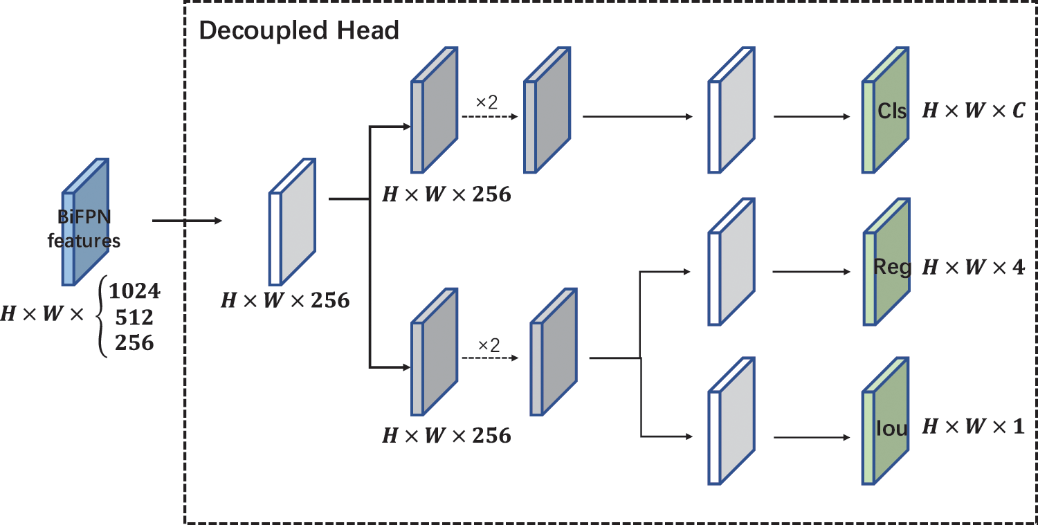
Figure 8: The structure of decoupled head

By stacking the three prediction results, each feature layer can obtain Out(h,w,4+1+num_classes) prediction information, including the position and category details of the prediction box. The prediction data must be decoded to get the final forecast result.

As the proposed vehicle detection model used in this paper is Anchor Free, the Decoupled Head directly predicts 4 target parameters of the bounding box [x,y,h,w] at each position. As shown in Fig. 9, these four parameters correspond to the offset of the predicted target centroid relative to the upper left corner (c) of the Grid Cell separately, and the width and height factors of the target. Note that these values are relative to the predicted feature map scale, if you want to map back to the original map you need to multiply the current feature map with the step size relative to the original map. The Anchor Free technique has the following advantages. (1) It requires less computational work, produces fewer prediction frames, and does not require IoU computation. (2) It solves the issue of positive and negative sample imbalance. (3) It does not require anchor adjustment.

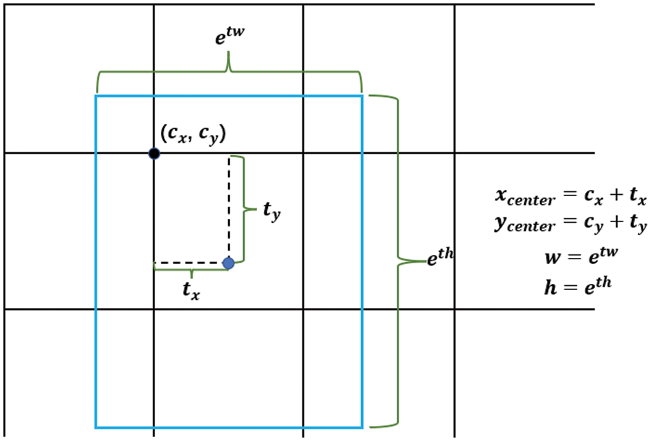
Figure 9: Anchor Free algorithm generates prediction frame

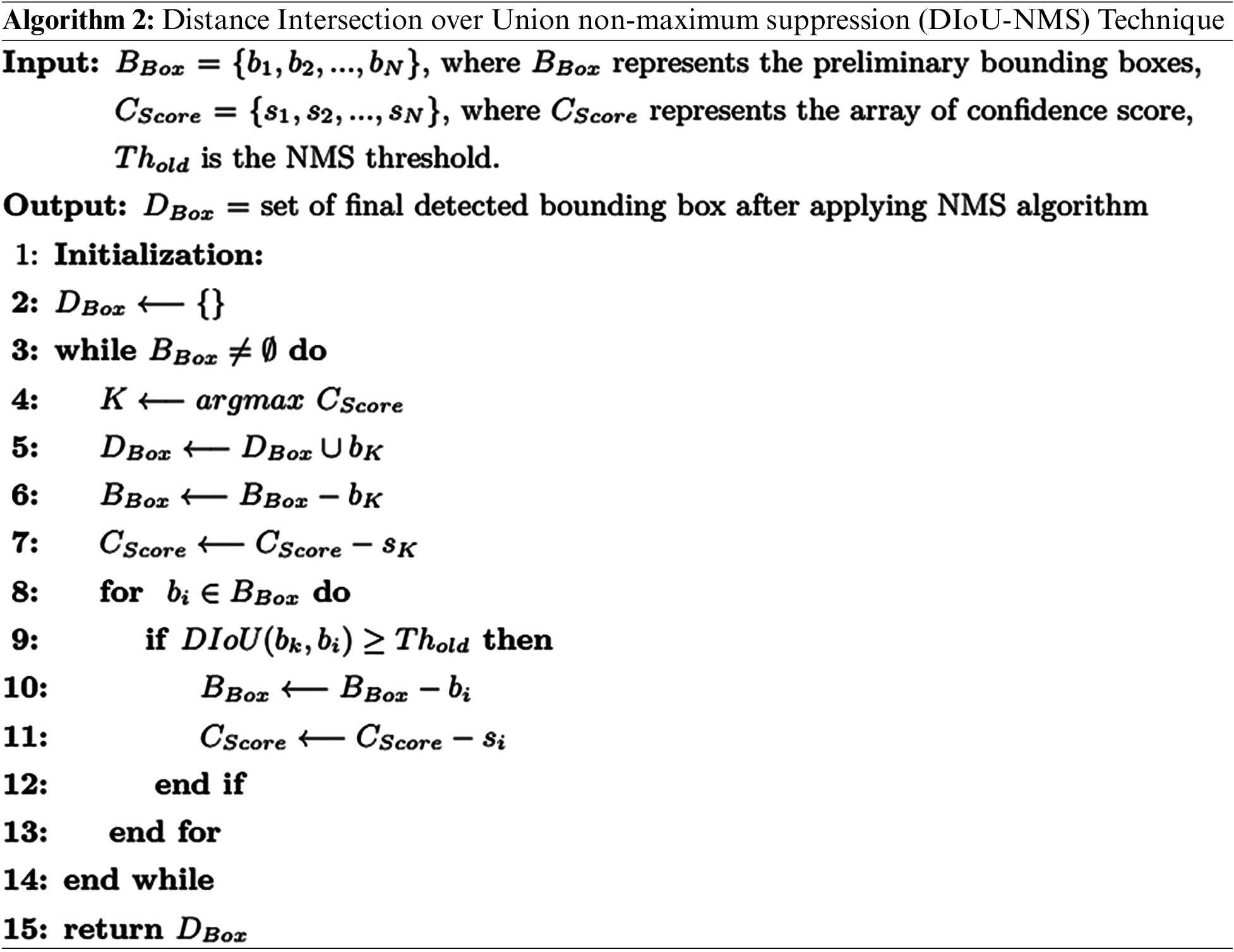
To choose a few detection boxes with a high level of confidence, filtering is first done based on the magnitude of the confidence. After filtering, remove the detection frames that repeatedly identify the same object in a certain location using the Distance Intersection over Union Non-Maximum Suppression (DIoU-NMS) approach. The IoU threshold in the Non-Maximum Suppression (NMS) algorithm will be replaced with Distance Intersection over Union (DIoU). The pseudo-code for the DIoU-NMS is shown in Algorithm 2. The DIoU is calculated by Eq. (5).

DIoU=IoU−Distance_22Distance_C2(5)

where Distance_2 represents the Euclidean distance between the center point of the predicted box and the real box, Distance_C the diagonal length of the smallest outer rectangle of the predicted box and the real box. The formula of IoU is shown in Eq. (6).

IoU=Intersection(box_p,box_gt)Union(box_p,box_gt)(6)

where box_p represents the predicted box, box_gt represents the real box. Intersection(box_p,box_gt) represents the size of the intersection area of the two boxes, Union(box_p,box_gt) represents the size of the union area of the two boxes.

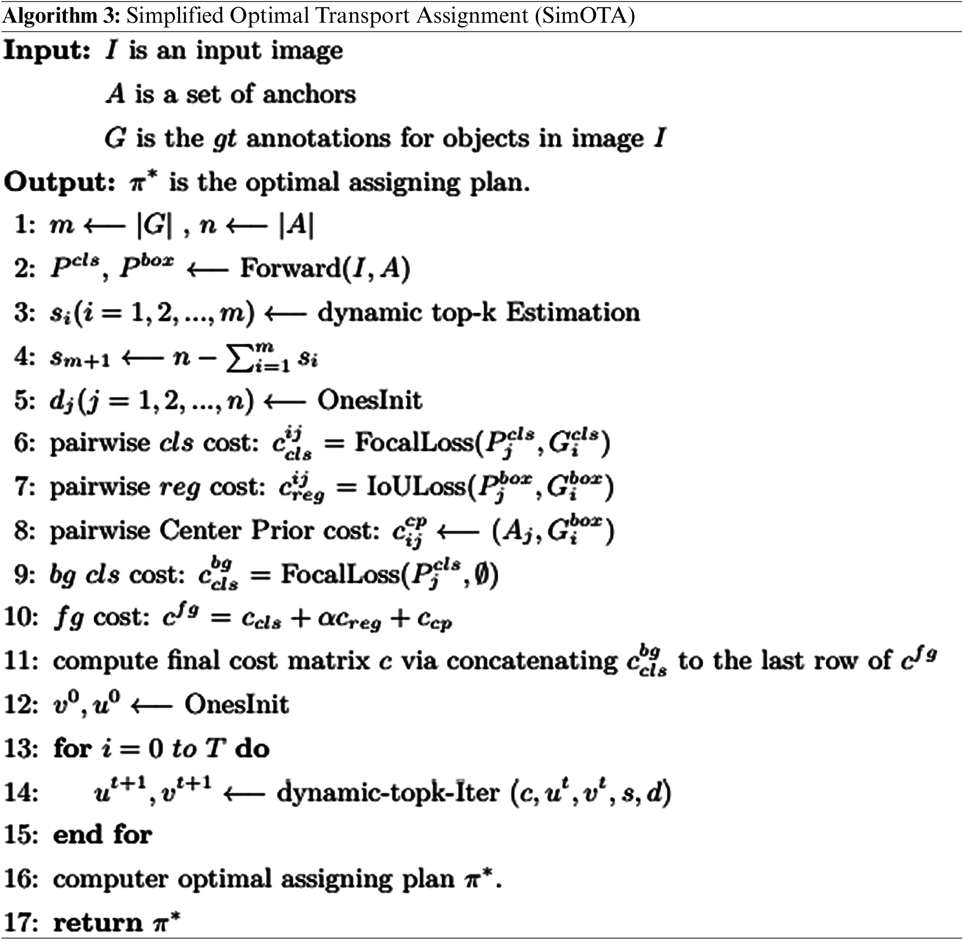
Finding the k anchor points with the lowest cost value in the cost matrix as the positive samples of the real frame is done during training using the SimOTA label matching approach. Eq. (7) illustrates the cost value calculation formula:

cij=Lijcls+λLijreg(7)

where Lijcls is the classification loss between each sample and real box, Lijreg is the regression loss between each sample and real box, λ is a constant that is usually set to 3. The next step is to choose the 10 positive samples with the biggest IoU value in the current real frame, add their IoU values, and round them down to k values. Varied real frames have different values for k, and the positive samples of the real frames are chosen from the k sample locations with the lowest cost values. The SimOTA algorithm’s main goal is to identify global prediction frames that matches all actual frames in the image with a high degree of confidence. This significantly reduces the multi-objective coupling problem that is prevalent in existing detection models. The pseudo code for the SimOTA is shown in Algorithm 3.

All positive samples and their associated real frames can be located after the aforementioned procedure is finished. The other anchor points are classified as negative samples. The Loss of the filtered positive samples is calculated in the following step. The Loss is mostly used to display the discrepancy between the expected and actual data, encompassing the three components of Reg, Obj, and Cls. The Loss is calculated as Eqs. (8)–(11):

Loss=1Npos(Lcls+λLreg+Lobj)(8)

Lcls=−∑i=1n∑j=1m(Oijlog(C^ij)+(1−Oij)log⁡(1−C^ij))(9)

Lreg=−log(IoU(box_p,box_gt))(10)

Lobj=−∑i=1n(oilog(c^i)+(1−oi)log⁡(1−c^i))(11)

where Lcls represents the classification loss; Lreg represents the localization loss; Lobj represents the confidence loss; λ represents the balance coefficient of localization loss, which is set to 5.0 in this model. Npos represents the number of positive samples filtered by the step of SimOTA. Oij∈{0,1} represents the existence or absence of the j-th class target in the i-th prediction box. The target probability that was obtained after being processed by the Sigmoid function is C^ij. The predicted frame’s confidence is represented by c^i, and the IoU between the predicted and actual frames is shown by oi. As the model is trained, the Loss value falls and the prediction of the positions and kinds of target objects gets more precise.

4  Experiments

4.1 Dataset

In this part, we assess the performance of the suggested model using the UA-DETRAC benchmark dataset [57,58]. The UA-DETRAC collection, which includes more than 80,000 actual road vehicle photos, was collected from road vehicles at 24 distinct sites in Beijing and Tianjin. These pictures were taken from more than 60 videos that included four clearly labeled target objects: car, bus, van, and other. Fig. 10 shows the distribution of parameters in the dataset. The target objects in the images have three kinds of status: fully visible, partially obscured, and truncated. Target object sizes can be divided into three categories: tiny (0–50 pixels), medium (50–150 pixels), and large (more than 150 pixels). The four different weather states portrayed in the dataset photographs are sunny, rainy, nocturnal, and cloudy. Examples of photos from the dataset are shown in Fig. 11.

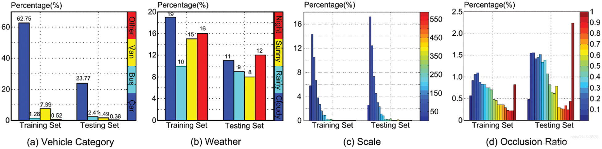
Figure 10: The parameters of the UA-DETRAC benchmark dataset

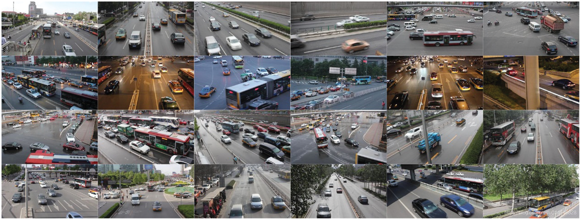
Figure 11: Examples of the UA-DETRAC benchmark dataset

All the models in this work are tested and trained using the same training set and test set, which are partitioned in this paper in a ratio of 2:1 between the training and test sets of the dataset.

4.2 Implementation Details

The input photos are scaled down during training such that their width and height are uniformly standardized to 640 * 640 pixels, and they are then fed into the target detection model. All models utilized in the experiments of this paper’s experiments had their pre-training weights acquired by training on the Common Objects in Context Train in the 2017 (COCO-Train2017) dataset. The total number of epochs is set to 60 during the training phase. The learning rate for the first 40 epochs is set to 10−4, the learning rate for the next 41 to 50 epochs is set to 10−5, and the learning rate of the last ten epochs is set to 10−6. In the network, the momentum decay and weight decay are set to 0.9 and 0.0005, respectively. Schedule the learning rate using the cosine annealing decay approach. Due to device constraints, multi-threaded data reading has been disabled. The confidence level is set to 0.5, the NMS IoU is set to 0.3, and the maximum number of prediction boxes that can be included in each picture is set to 100 during the test. MINOVERLAP is set to 0.5 to produce mAP0.5. The model parameters are modified during the experiment using the Adam optimizer. The RTX-2080ti Graphic Processing Unit (GPU) was used to accomplish all experiments.

4.3 Evaluation Metrics

The Average Precision (AP) of each category and Mean Average Precision (mAP) [59–61] are selected as the accuracy performance index because the proposed model in this paper is created to adapt to target detection in complex traffic circumstances. Eqs. (12)–(15) calculates the AP and mAP.

P=TP/(TP+FP)(12)

R=TP/(TP+FN)(13)

AP=∫01P(R)dR(14)

mAP=1|QR|∑q∈QRAP(q)(15)

where TP,TN,FP,FN represent the value of True Positive, True Negative, False Positive, and False Negative, respectively. P denotes the percentage of correctly predicted positive samples in all positively predicted samples, and R denotes the percentage of correctly predicted positive samples in all positive samples. |QR| denotes the quantity of target categories, q represents the type of detected target, and AP(q) represents the AP of the category q.

The speed evaluation metric is the detecting speed Frame Per Second (FPS). Numbers of model Parameters (Params) and model computation amount are used as evaluation metrics to assess the model’s complexity.

5  Experimental Results

5.1 Comparison of Indicators

The performance of the proposed vehicle detection model and other popular vehicle detection models are compared in this section using the same experimental setup. Map and AP for several models are included in Table 1 for comparison. The computation amount for each model is shown in Table 2 along with the number of parameters.

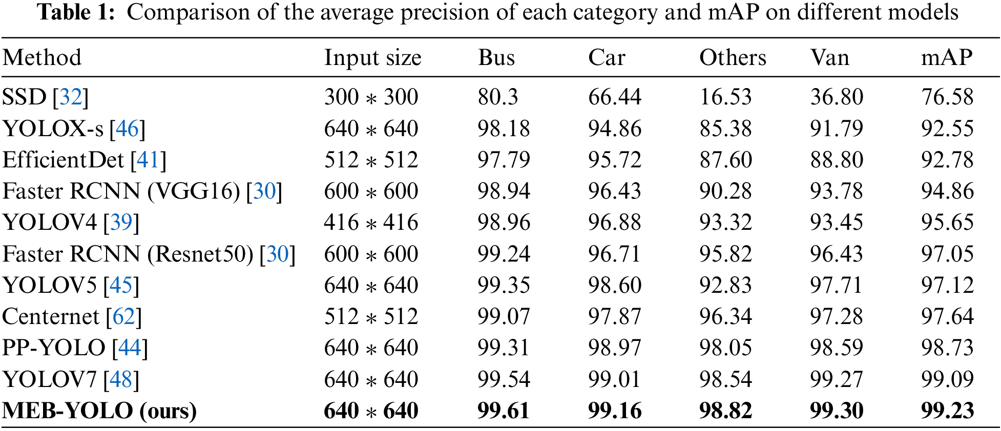
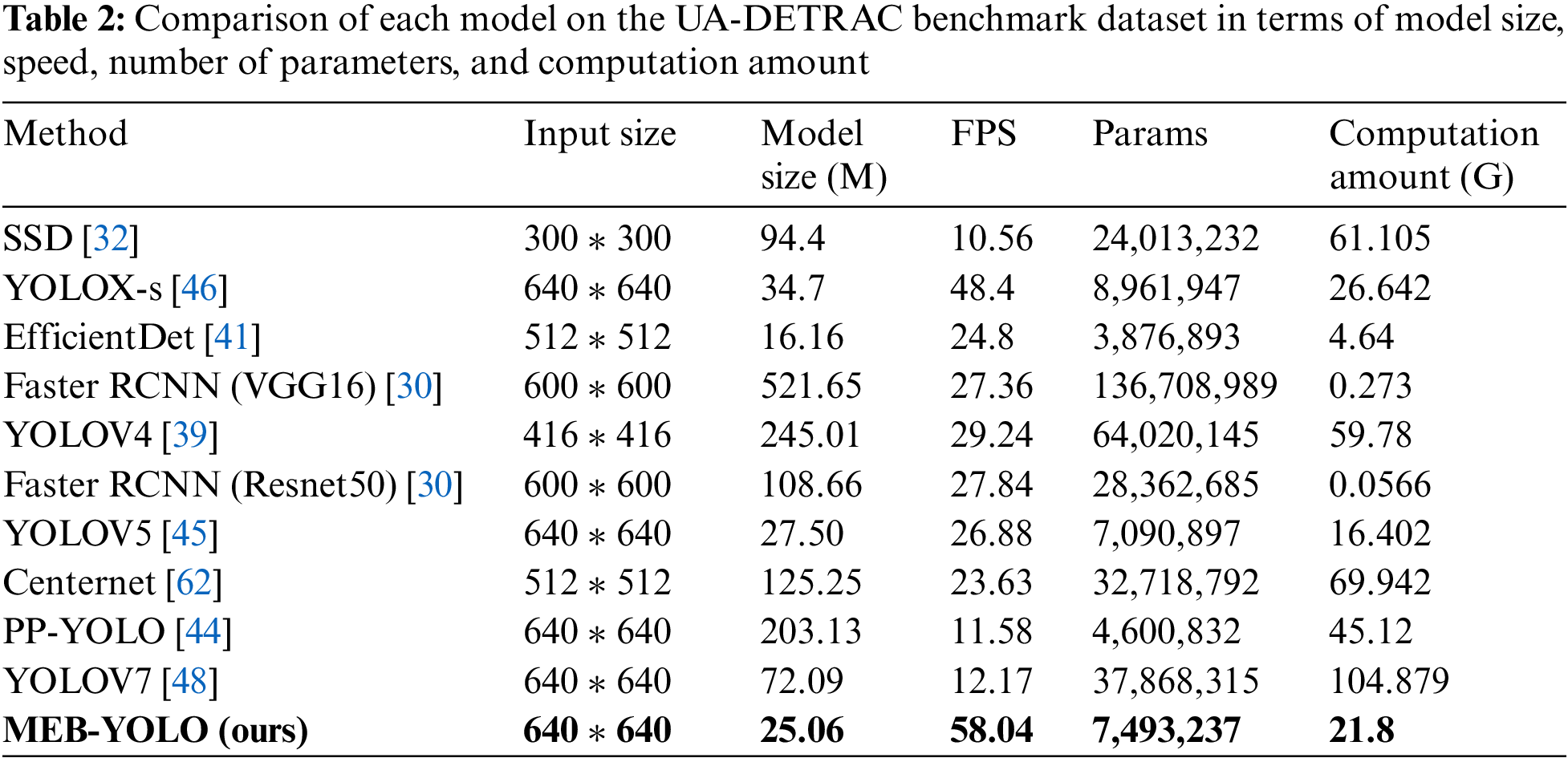
Table 1 shows that the MEB-YOLO model proposed in this paper improves the mAP by 6.6% compared to the YOLOX-s model, 29.6% compared to the SSD model, 7.0% compared to the EfficientDet model, 2.2% compared to the Faster RCNN (Resnet50) model, 4.6% compared to the Faster RCNN (VGG16) model, 3.7% compared to the YOLOV4 model, 2.2% compared to the YOLOV5 model, 1.6% compared to the Centernet model, 0.5% compared to the PP-YOLO model, 0.14% compared to the YOLOV7model. Overall, mAP and the AP of the four vehicle types outperform the compared algorithms.

Table 2 shows that the proposed model has 9.76 higher FPS, 9.64M less model size, 1,468,710 fewer parameters, and 4.842G lower computation than the YOLOX-s model. Speed, accuracy, model memory capacity, time complexity, and spatial complexity are all improved by the proposed model over the YOLOX-s model. The proposed model achieves a mix of high speed and high accuracy thanks to its detection speed, which is also noticeably faster than the methods that were examined. The proposed model uses less memory and has less computation and parameters than the other models that were compared.

Even though the proposed model’s time complexity and spatial complexity trail behind the EfficientDet and the Faster RCNN model, respectively, it performs rather well overall. Although the proposed model has fewer parameters and requires slightly more computation amount than the EfficientDet, it is more accurate and faster, which is very advantageous for real-time vehicle identification. As a result, the proposed model increases detection speed while maintaining accuracy, is more robust when recognizing small targets in challenging traffic scenarios, and is more efficient.

5.2 Comparison of Visualization Results

The MEB-YOLO model and the YOLOX-s model’s results for detecting automobiles in certain test photos are compared in Fig. 12. Where the MEB-YOLO model for detecting vehicles yielded the following results (a), (c), (e), (g), (i), (k), whereas the YOLOX-s model yielded the following results (b), (d), (f), (h), (j), (l). While the YOLOX-s model fails to identify the vehicle indicated by the pink arrow in Fig. 12b, our model properly recognizes it as a truck in Fig. 12a. The MEB-YOLO model successfully detects small cars in the distance in Figs. 12c and 12e. While the far-off vehicle targets marked in pink in Figs. 12d and 12f are not picked up by the YOLOX-s model’s prediction results. In Fig. 12g, the MEB-YOLO model properly identifies the “van” denoted by the pink arrow in Fig. 12h, but the YOLOX-s model misidentifies it as the category of “vehicle”. When comparing Figs. 12i and 12j, it can be seen that the results of the two models’ detection do not significantly differ from one another and that both have a higher detection rate in low-light situations at night. The MEB-YOLO model, on the other hand, has a better confidence level in accurately detecting the target, and the size of the detection frame is more in line with the outline of the actual automobiles in the image. The road photos in Figs. 12k and 12l depict an evening scene where streetlights are out but car headlights are on. The photos have low-resolution pixels and poor lighting. The MEB-YOLO model is superior to the YOLOX-s model at detecting small target vehicles at the range indicated by the pink circle in Fig. 12l. As a result, we may conclude that the proposed model can more accurately recognize small targets and detect targets at a distance. Additionally, the targets that the YOLOX-s model missed or wrongly detected are correctly identified by the MEB-YOLO model. This shows that the suggested model has improved detection accuracy for small targets, as well as in ambiguous and low-light conditions.

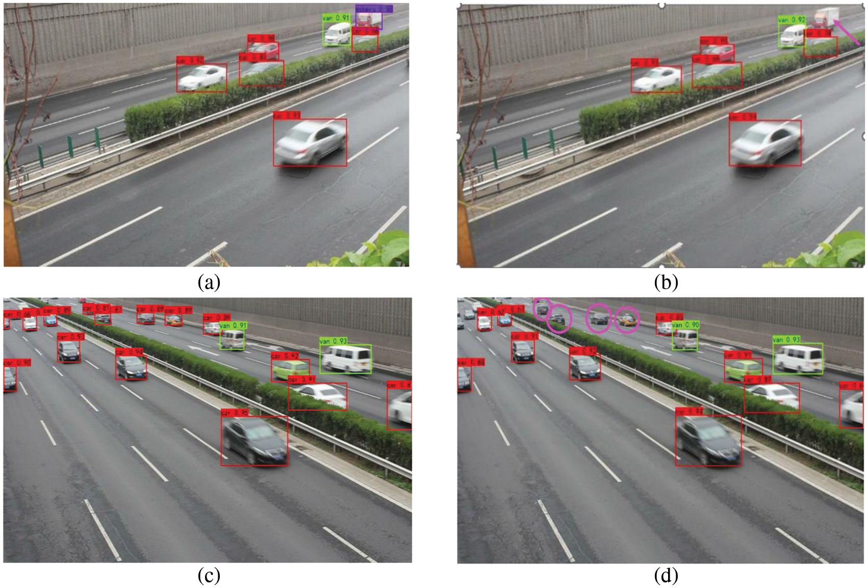
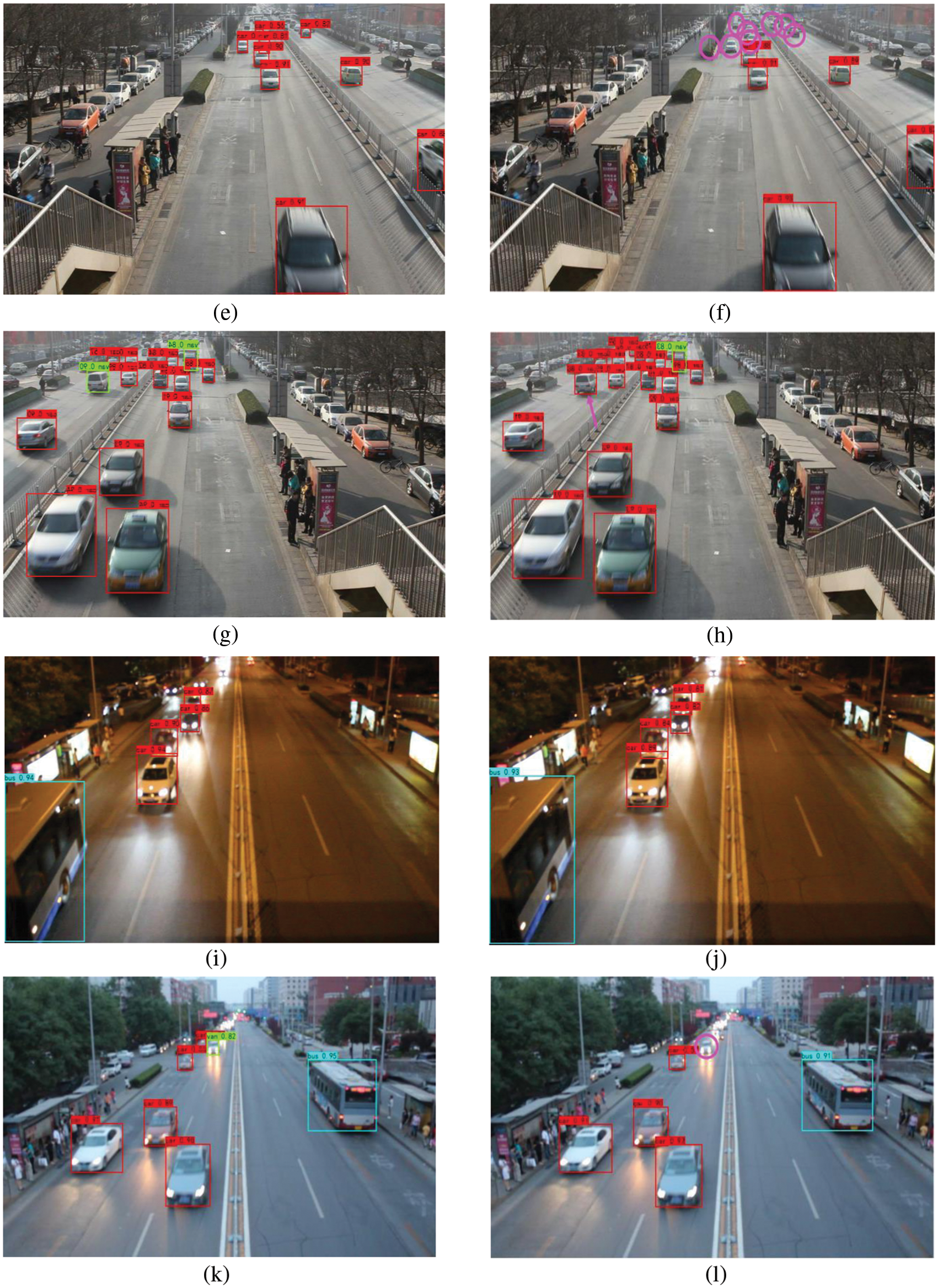
Figure 12: Comparison of the detection results obtained from the proposed MEB-YOLO model and the YOLOX-s model in different environments

6  Conclusion

For efficient vehicle detection in complicated traffic scenarios, a novel detection model named MEB-YOLO is proposed in this paper. To increase the robustness of the network model for tiny and multiple target detection in complex traffic situations, Mosaic and MixUp data enhancement methods are used to preprocess the dataset. To enhance the network’s ability to extract features from the foreground target, the ECA attention mechanism and ACON activation function is utilized to reconstruct the Backbone network, somewhat mitigating the detrimental effects of the complex background, allowing the model to concentrate more on the target than the background. To achieve the fusion of more high-level features, the BiFPN is employed as the structure of the Neck network to drastically minimize the model’s size, memory, and complexity. Decoupled Head, Anchor Free approach, and SimOTA are used in the Prediction module to get the final forecast results. Convergence of these technologies accelerates the model convergence speed and improves the model accuracy, reduces the computational volume, decreases the computational cost, and resolves the positive and negative sample imbalance problem, cuts down on training time. The experimental results demonstrate that the proposed method outperforms the state-of-the-art (SOTA) target detection models in terms of target detection accuracy and target detection speed. It can satisfy the demand for real-time, accurate, and high-speed target detection of road traffic images. Even in low-resolution photos, the target vehicle can be spotted more precisely and has produced promising results in detecting small targets.

However, the proposed method in this paper still has some shortcomings. For example, the detection effectiveness of our proposed model is affected when the road images obtained by the camera are not too clear. In addition, we failed to deploy the model on mobile devices such as cell phones because the computational capability of our proposed model is still relatively high. In future research, we will continue to improve our model using saliency detection or remote sensing image target detection and transfer it to an embedded platform to integrate with systems such as vehicle tracking and traffic flow estimation.

Funding Statement: This work is partially funded by the National Natural Science Foundation of China (NSFC) (No. 61170110), Zhejiang Provincial Natural Science Foundation of China (LY13F020043).

Conflicts of Interest: The authors declare that they have no conflicts of interest to report regarding the present studies.

References

1. S. Razakarivony and F. Jurie, “Vehicle detection in aerial imagery: A small target detection benchmark,” Journal of Visual Communication and Image Representation, vol. 34, no. 1, pp. 187–203, 2016. [Google Scholar]
2. F. Hong, C. Lu, C. Liu, R. R. Liu and J. Wei, “A traffic surveillance multi-scale vehicle detection object method base on encoder-decoder,” IEEE Access, vol. 8, no. 1, pp. 47664–47674, 2016. [Google Scholar]
3. X. Liu and Z. Zhang, “A vision-based target detection, tracking, and positioning algorithm for unmanned aerial vehicle,” Wireless Communications and Mobile Computing, vol. 2021, no. 7, pp. 1–12, 2021. [Google Scholar]
4. K. Wang, Z. Meng and Z. Wu, “Deep learning-based ground target detection and tracking for aerial photography from UAVs,” Applied Sciences, vol. 11, no. 18, pp. 8434, 2021. [Google Scholar]
5. G. Dimitrakopoulos and P. Demestichas, “Intelligent transportation systems,” IEEE Vehicular Technology Magazine, vol. 5, no. 1, pp. 77–84, 2010. [Google Scholar]
6. C. Luo, X. Yang and A. Yuille, “Self-supervised pillar motion learning for autonomous driving,” in Proc. of the IEEE/CVF Conf. on Computer Vision and Pattern Recognition, Seattle, WA, USA, pp. 3183–3192, 2021. [Google Scholar]
7. M. Schwarzinger, T. Zielke, D. Noll, M. Brauckmann and W. Von Seelen, “Vision-based car-following: Detection, tracking, and identification,” in Proc. of the Intelligent Vehicles92 Symp., Detroit, MI, USA, pp. 24–29, 1992. [Google Scholar]
8. A. Voulodimos, N. Doulamis, A. Doulamis and E. Protopapadakis, “Deep learning for computer vision: A brief review,” Computational Intelligence and Neuroscience, vol. 2018, pp. 1–13, 2018. [Google Scholar]
9. Q. Fan, L. Brown and J. Smith, “A closer look at faster R-CNN for vehicle detection,” in 2016 IEEE Intelligent Vehicles Symp. (IV), Gothenburg, Sweden, pp. 124–129, 2016. [Google Scholar]
10. Z. Cai and N. Vasconcelos, “Cascade R-CNN: Delving into high quality object detection,” in Proc. of the IEEE Conf. on Computer Vision and Pattern Recognition, Salt Lake City, UT, USA, pp. 6154–6162, 2018. [Google Scholar]
11. X. Cheng, G. Qiu, Y. Jiang and Z. Zhao, “An improved small object detection method based on Yolo V3,” Pattern Analysis and Applications, vol. 24, no. 3, pp. 1347–1355, 2001. [Google Scholar]
12. M. Abdelwahab, M. Abdel-Nasser and R. Taniguchi, “Efficient and fast traffic congestion classification based on video dynamics and deep residual network,” in Int. Workshop on Frontiers of Computer Vision, Singapore, pp. 3–17, 2020. [Google Scholar]
13. X. Ding and R. Yang, “Vehicle and parking space detection based on improved yolo network model,” Journal of Physics: Conference Series, vol. 1325, no. 1, pp. 012084, 2019. [Google Scholar]
14. T. Doan and M. Truong, “Real-time vehicle detection and counting based on YOLO and DeepSORT,” in 2020 12th Int. Conf. on Knowledge and Systems Engineering (KSE), Can Tho, Vietnam, pp. 67–72, 2020. [Google Scholar]
15. B. Xu, B. Wang and Y. Gu, “Vehicle detection in aerial images using modified YOLO,” in 2019 IEEE 19th Int. Conf. on Communication Technology (ICCT), Xi’an, China, pp. 1669–1672, 2020. [Google Scholar]
16. J. Azimjonov and A. Zmen, “A real-time vehicle detection and a novel vehicle tracking systems for estimating and monitoring traffic flow on highways,” Advanced Engineering Informatics, vol. 50, no. 1, pp. 101393, 2021. [Google Scholar]
17. D. Carrasco, H. Rashwan, M. García and D. Puig, “T-YOLO: Tiny vehicle detection based on YOLO and multi-scale convolutional neural networks,” IEEE Access, vol. 11, pp. 22430–22440, 2021. [Google Scholar]
18. Z. Hou, J. Yan, B. Yang and Z. Ding, “A novel UAV aerial vehicle detection method based on attention mechanism and multi-scale feature cross fusion,” in 2021 2nd Int. Conf. on Artificial Intelligence in Electronics Engineering, Guangzhou, China, pp. 51–59, 2021. [Google Scholar]
19. X. Xu, X. Zhang, T. Zhang, Z. Yang, J. Shi et al., “Shadow-background-noise 3D spatial decomposition using sparse low-rank gaussian properties for video-SAR moving target shadow enhancement,” IEEE Geoscience and Remote Sensing Letters, vol. 19, pp. 1–5, 2022. [Google Scholar]
20. S. Chen and W. Lin, “Embedded system real-time vehicle detection based on improved YOLO network,” in 2019 IEEE 3rd Advanced Information Management, Communicates, Electronic and Automation Control Conf. (IMCEC), Chongqing, China, pp. 1400–1403, 2019. [Google Scholar]
21. K. E. Van de Sande, J. R. Uijlings, T. Gevers and A. W. Smeulders, “Segmentation as selective search for object recognition,” International Journal of Computer Vision, vol. 104, no. 2, pp. 154–171, 2011. [Google Scholar]
22. P. Viola and M. Jones, “Rapid objection detection using a boosted cascade of simple features,” in IEEE Conf. on Computer Vision and Pattern Recognition, Kauai, HI, USA, pp. 511–518, 2001. [Google Scholar]
23. N. Dalal and B. Triggs, “Histograms of oriented gradients for human detection,” IEEE Computer Society Conference on Computer Vision and Pattern Recognition, vol. 2, no. 1, pp. 886–893, 2005. [Google Scholar]
24. D. G. Lowe, “Distinctive image features from scale-invariant keypoints,” International Journal of Computer Vision, vol. 60, no. 2, pp. 91–110, 2004. [Google Scholar]
25. S. R. Gunn, “Support vector machines for classification and regression,” ISIS Technical Report, vol. 14, no. 1, pp. 5–16, 1998. [Google Scholar]
26. L. Huang, W. Pan, Y. Zhang, L. Qian, N. Ga et al., “Data augmentation for deep learning-based radio modulation classification,” IEEE Access, vol. 8, no. 1, pp. 1498–1506, 2019. [Google Scholar]
27. L. Zuo, H. Sun, Q. Miao, R. Qi and R. Jia, “Natural scene text recognition based on Encoder-Decoder framework,” IEEE Access, vol. 7, no. 1, pp. 62616–62623, 2019. [Google Scholar]
28. Q. Mao, H. Sun, Y. Liu and R. Jia, “Fast and efficient non-contact ball detector for picking robots,” IEEE Access, vol. 7, pp. 175487–175498, 2019. [Google Scholar]
29. R. Girshick, J. Donahue, T. Darrell and J. Malik, “Rich feature hierarchies for accurate object detection and semantic segmentation,” in Proc. of the IEEE Conf. on Computer Vision and Pattern Recognition (CVPR), Columbus, OH, USA, pp. 580–587, 2014. [Google Scholar]
30. S. Ren, K. He, R. Girshick and J. Sun, “Faster R-CNN: Towards real-time object detection with region proposal networks,” IEEE Transactions on Pattern Analysis & Machine Intelligence, vol. 39, no. 6, pp. 1137–1149, 2017. [Google Scholar]
31. A. Koirala, K. Walsh, Z. Wang and C. McCarthy, “Deep learning for real-time fruit detection and orchard fruit load estimation: Benchmarking of ‘MangoYOLO’,” Precision Agriculture, vol. 20, no. 6, pp. 1107–1135, 2019. [Google Scholar]
32. W. Liu, D. Anguelov, D. Erhan, C. Szegedy, S. Reed et al., “SSD: Single shot multibox detector,” in European Conf. on Computer Vision, Amsterdam, Netherlands, pp. 21–37, 2016. [Google Scholar]
33. J. Sang, Z. Wu, P. Guo, H. Hu, H. Xiang et al., “An improved YOLOv2 for vehicle detection,” Sensors, vol. 18, no. 12, pp. 4272, 2018. [Google Scholar] [PubMed]
34. J. Redmon and A. Farhadi, YOLOv3: An incremental improvement. Computer Vision and Pattern Recognition, 2018. [Online]. Available: https://arxiv.org/abs/1804.02767 [Google Scholar]
35. M. A. Al-qaness, A. A. Abbasi, H. Fan, R. A. Ibrahim, S. H. Alsamhi et al., “An improved YOLO-based road traffic monitoring system,” Computing, vol. 103, pp. 211–230, 2021. [Google Scholar]
36. Y. Lecun and L. Bottou, “Gradient-based learning applied to document recognition,” Proceedings of the IEEE, vol. 86, no. 11, pp. 2278–2324, 1998. [Google Scholar]
37. A. Krizhevsky, I. Sutskever and G. Hinton, “ImageNet classification with deep convolutional neural networks,” Communications of the ACM, vol. 60, no. 6, pp. 84–90, 2017. [Google Scholar]
38. K. He, X. Zhang, S. Ren and J. Sun, “Spatial pyramid pooling in deep convolutional networks for visual recognition,” IEEE Transactions on Pattern Analysis and Machine Intelligence, vol. 37, no. 9, pp. 1904–1916, 2015. [Google Scholar] [PubMed]
39. A. Bochkovskiy, C. Wang and H. Liao, YOLOv4: Optimal speed and accuracy of object detection. Computer Vision and Pattern Recognition, 2020. [Online]. Available: https://arxiv.org/abs/2004.10934 [Google Scholar]
40. H. Law and J. Deng, “CornerNet: Detecting objects as paired keypoints,” International Journal of Computer Vision, vol. 128, no. 3, pp. 642–656, 2020. [Google Scholar]
41. M. Tan, R. Pang and Q. Le, “EfficientDet: Scalable and efficient object detection,” in Proc. of the IEEE/CVF Conf. on Computer Vision and Pattern Recognition (CVPR), Seattle, WA, USA, pp. 10781–10790, 2020. [Google Scholar]
42. X. Zhao, F. Pu, Z. Wang, H. Chen and Z. Xu, “Detection, tracking, and geolocation of moving vehicle from UAV using monocular camera,” IEEE Access, vol. 7, pp. 101160–101170, 2019. [Google Scholar]
43. Z. Liu, Y. Lin, Y. Cao, H. Hu, Y. Wei et al., “Swin transformer: Hierarchical vision transformer using shifted windows,” in Proc. of the IEEE/CVF Int. Conf. on Computer Vision (ICCV), Montreal, Canada, pp. 10012–10022, 2021. [Google Scholar]
44. X. Long, K. Deng, G. Wang, Y. Zhang, Q. Dang et al., PP-YOLO: An effective and efficient implementation of object detector, 2020. [Online]. Available: https://doi.org/10.48550/arXiv.2007.12099 [Google Scholar] [CrossRef]
45. G. Yang, W. Feng, J. Jin, Q. Lei, X. Li et al., “Face mask recognition system with YOLOV5 based on image recognition,” in 2020 IEEE 6th Int. Conf. on Computer and Communications (ICCC), Chengdu, China, pp. 1398–1404, 2020. [Google Scholar]
46. Z. Ge, S. Liu, F. Wang, Z. Li and J. Sun, YOLOX: Exceeding YOLO series in 2021. Computer Vision and Pattern Recognition, 2021. [Online]. Available: https://arxiv.org/abs/2107.08430 [Google Scholar]
47. X. Xu, X. Zhang and T. Zhang, “Lite-YOLOV5: A lightweight deep learning detector for on-board ship detection in large-scene sentinel-1 sar images,” Remote Sensing, vol. 14, no. 4, pp. 1018, 2022. [Google Scholar]
48. C. Y. Wang, A. Bochkovskiy and H. Y. M. Liao, YOLOv7: Trainable bag-of-freebies sets new state-of-the-art for real-time object detectors, 2022.[Online]. Available: https://doi.org/10.48550/arXiv.2207.02696 [Google Scholar] [CrossRef]
49. X. Xu, Y. Jiang, W. Chen, Y. Huang, Y. Zhang et al., DAMO-YOLO: A Report on Real-Time Object Detection Design, 2022. [Online]. Available: https://doi.org/10.48550/arXiv.2211.15444 [Google Scholar] [CrossRef]
50. D. Zhang, D. Meng and J. Han, “Co-saliency detection via a self-paced multiple-instance learning framework,” IEEE Transactions on Pattern Analysis and Machine Intelligence, vol. 39, no. 5, pp. 865–878, 2016. [Google Scholar] [PubMed]
51. C. Wang, S. Dong, X. Zhao, G. Papanastasiou, H. Zhang et al., “SaliencyGAN: Deep learning semi-supervised salient object detection in the fog of IoT,” IEEE Transactions on Industrial Informatics, vol. 16, no. 4, pp. 2667–2676, 2019. [Google Scholar]
52. S. Woo, J. Park, J. Lee and I. S. Kweon, “CBAM: Convolutional block attention module,” in Proc. of the European Conf. on Computer Vision (ECCV), Munich, Germany, pp. 3–19, 2018. [Google Scholar]
53. J. Hu, L. Shen and G. Sun, “Squeeze-and-excitation networks,” in Proc. of the IEEE Conf. on Computer Vision and Pattern Recognition, pp. 7132–7141, 2018. [Google Scholar]
54. Q. Wang, B. Wu, P. Zhu, P. Li, W. Zuo et al., “ECA-Net: Efficient channel attention for deep convolutional neural networks,” in IEEE/CVF Conf. on Computer Vision and Pattern Recognition (CVPR), Seattle, WA, USA, pp. 11534–11542, 2020. [Google Scholar]
55. Y. Wang, C. Hua, W. Ding and R. Wu, “Real-time detection of flame and smoke using an improved YOLOv4 network,” Signal, Image and Video Processing, vol. 16, no. 4, pp. 1109–1116, 2020. [Google Scholar]
56. A. Joulin, M. Cissé, D. Grangier and H. Jégou, “Efficient softmax approximation for GPUs,” in Proc. of the 34th Int. Conf. on Machine Learning, vol. 70, pp. 1302–1310, 2017. [Google Scholar]
57. S. Lyu, M. C. Chang, D. Du, L. Wen, H. Qi et al., “UA-DETRAC 2017: Report of AVSS2017 & IWT4S challenge on advanced traffic monitoring,” in 2017 14th IEEE Int. Conf. on Advanced Video and Signal Based Surveillance (AVSS), Agrigento, Italy, pp. 1–7, 2017. [Google Scholar]
58. L. Wen, D. Du, Z. Cai, Z. Lei, M. C. Chang et al., “UA-DETRAC: A new benchmark and protocol for multi-object detection and tracking,” Computer Vision and Image Understanding, vol. 193, no. 9, pp. 102707, 2020. [Google Scholar]
59. M. Everingham, L. Van Gool, C. K. Williams, J. Winn and A. Zisserman, “The pascal visual object classes (VOC) challenge,” International Journal of Computer Vision, vol. 88, no. 2, pp. 303–338, 2010. [Google Scholar]
60. M. Everingham, S. Eslami, L. Van Gool, C. K. Williams and J. Winn, “The pascal visual object classes challenge: A retrospective,” International Journal of Computer Vision, vol. 111, no. 1, pp. 98–136, 2015. [Google Scholar]
61. O. Russakovsky, J. Deng, H. Su, J. Krause, S. Satheesh et al., “ImageNet large scale visual recognition challenge,” International Journal of Computer Vision, vol. 115, no. 3, pp. 211–252, 2015. [Google Scholar]
62. K. Duan, S. Bai, L. Xie, H. Qi, Q. Huang et al., “CenterNet: Keypoint triplets for object detection,” in 2009 IEEE/CVF Int. Conf. on Computer Vision (ICCV), Seoul, Korea, pp. 6569–6578, 2019. [Google Scholar]
Cite This Article
Copyright © 2023 The Author(s). Published by Tech Science Press.
This work is licensed under a Creative Commons Attribution 4.0 International License , which permits unrestricted use, distribution, and reproduction in any medium, provided the original work is properly cited.
Downloads
Citation Tools