
 Submit a Paper
 Propose a Special lssue
 Open Access
ARTICLE
Exact Solutions and Finite Time Stability of Linear Conformable Fractional Systems with Pure Delay
1
School of Mathematics, Harbin Institute of Technology, Harbin, 150001, China
2
Department of Mathematics, Faculty of Science, Mansoura University, Mansoura, 35516, Egypt
3
Mathematical Science Department, Faculty of Science, Princess Nourah Bint Abdulrahman University,
Riyadh, 11546, Saudi Arabia
4
Section of Mathematics, International Telematic University Uninettuno, Roma, 00186, Italy
* Corresponding Authors: Ahmed M. Elshenhab. Email: ; Omar Bazighifan. Email:
Computer Modeling in Engineering & Sciences 2023, 134(2), 927-940. https://doi.org/10.32604/cmes.2022.021512
Received 18 January 2022; Accepted 23 March 2022; Issue published 31 August 2022
 View Full Text
 Download PDF
Abstract
We study nonhomogeneous systems of linear conformable fractional differential equations with pure delay. By using new conformable delayed matrix functions and the method of variation, we obtain a representation of their solutions. As an application, we derive a finite time stability result using the representation of solutions and a norm estimation of the conformable delayed matrix functions. The obtained results are new, and they extend and improve some existing ones. Finally, an example is presented to illustrate the validity of our theoretical results.Keywords
In recent years, particularly in 2014, Khalil et al. [1] introduced a new definition of the fractional derivative called the conformable fractional derivative that extends the classical limit definition of the derivative of a function. The conformable fractional derivative has main advantages compared with other previous definitions. It can, for example, be used to solve the differential equations and systems exactly and numerically easily and efficiently, it satisfies the product rule and quotient rule, it has results similar to known theorems in classical calculus, and applications for conformable differential equations in a variety of fields have been extensively studied, see [2–10] and the references therein. On the other hand, in 2003, Khusainov et al. [11] represented the solutions of linear delay differential equations by constructing a new concept of a delayed exponential matrix function. In 2008, Khusainov et al. [12] adopted this approach to represent the solutions of an oscillating system with pure delay by establishing a delayed matrix sine and a delayed matrix cosine. This pioneering research yielded plenty of novel results on the representation of solutions, which are applied in the stability analysis and control problems of time-delay systems; see for example [13–28] and the references therein. Thereafter, in 2021, Xiao et al. [29] obtained the exact solutions of linear conformable fractional delay differential equations of order
However, to the best of our knowledge, no study exists dealing with the representation and stability of solutions of conformable fractional delay differential systems of order
Motivated by these papers, we consider the explicit formula of solutions of linear conformable fractional differential equations with pure delay
by constructing new conformable delayed matrix functions. Moreover, the representation of solutions of Eq. (1) is used to obtain a finite time stability result on
The paper is organized as follows: In Section 2, we present some basic definitions concerning conformable fractional derivative and finite time stability, and construct new conformable delayed matrix functions and derive their properties for use when we discuss the representation of solutions and finite time stability. In Section 3, by using the new conformable delayed matrix functions, we give the explicit formula of solutions of Eq. (1). In Section 4, as an application, we derive a finite time stability result using the representation of solutions. Finally, we give an example to illustrate the main results.
Throughout the paper, we denote the vector norm and matrix norm, respectively, as
We recall some basic definitions of conformable fractional derivative, fractional exponential function, and finite time stability.
Definition 2.1. ([2, Definition 2.2]). Let
if the limit exists.
Remark 2.1. As a consequence of Definition 2.1, we can show that
where
Definition 2.2. ([2]). We define the fractional exponential function as follows:
Definition 2.3. ([30]). The system in Eq. (1) is finite time stable with respect to
Next, we construct new conformable delayed matrix functions that are the fundamental solution matrices of Eq. (1).
Definition 2.4. The conformable delayed matrix functions
respectively, where
Lemma 2.1. The following rule is true:
Proof. First, when
Applying Remark 2.1, we get
This completes the proof.
In the same way that we proved Lemma 2.1, we can derive the next result.
Lemma 2.2. The following rule is true:
To conclude this section, we provide a norm estimation of the conformable delayed matrix functions, which is used while discussing finite time stability.
Lemma 2.3. For any
Proof. Taking the norm of Eq. (2), we get
This completes the proof.
Lemma 2.4. For any
Proof. Taking the norm of Eq. (3), we get
This completes the proof.
3 Exact Solutions for Linear Conformable Fractional Delay Systems
In this section, we give the exact solutions of Eq. (1) via the conformable delayed matrix functions and the method of variation of constants. To do this, we consider the homogeneous system of linear conformable fractional delay differential equations
and the linear inhomogeneous conformable fractional delay system
Theorem 3.1. The solution
Proof. We seek for a solution of Eq. (4) in the form
or
where
and
Consider Eq. (8). If
and
which implies that
and
Substituting Eq. (11) into Eq. (10), we get
Differentiating Eq. (12) with respect to x, we have
As a result, we find that the equalities obtained Eqs. (12) and (13) are true if
Substituting Eq. (14) into Eq. (7), we obtain Eq. (6). This finishes the proof.
Theorem 3.2. The particular solution
Proof. We try to find a particular solution
by applying the method of variation of constants, where
Substituting Eqs. (16) and (17) into Eq. (5), and noting that
We have
Corollary 3.1. The solution
Remark 3.1. Let
Remark 3.2. Let
where
4 Finite Time Stability of Linear Conformable Fractional Delay Systems
In this section, we establish some sufficient conditions for the finite time stability results of Eq. (1) by using a norm estimation of the conformable delayed matrix functions and the formula of general solutions of Eq. (1).
Theorem 4.1. The system Eq. (1) is finite time stable with respect to
Proof. By using Definition 2.3, and Theorems 3.1 and 3.2, we have
Note that
Thus
Therefore, from Lemma 2.4, we have
for
From Lemma 2.4, we have
From Eqs. (20), (22) and (23), we get
for all
Corollary 4.1. Let
is finite time stable with respect to
Remark 4.1. Let
Consider the conformable delay differential equations
where
From Theorems 3.1 and 3.2, for all
which implies that
and
where
and
Thus the explicit solutions of Eq. (25) are
where
and
where
By calculating we obtain
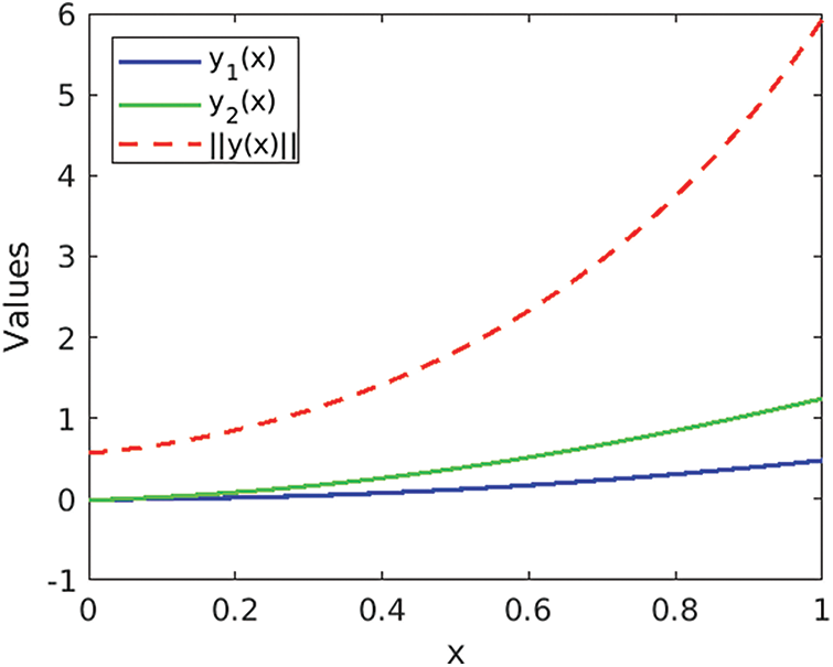
Figure 1: The state y(x) and ||y(x)|| of Eq. (25)
In this work, using new conformable delayed matrix functions, we derived explicit solutions of linear conformable fractional delay systems of order
Following the topic of this paper, we outline some possible next research directions. The first direction will include applying the results of this paper on control problems for conformable fractional delay systems of order
which lead to new results on stability and control problems. Depending on these results and delayed arguments, we will try to prove a generalized Lyapunov-type inequality for the conformable and sequential conformable boundary value problems
and
which leads to new results on the conformable Sturm-Liouville eigenvalue problem.
Acknowledgement: The authors would like to thank Princess Nourah bint Abdulrahman University Researchers Supporting Project No. (PNURSP2022R27), Princess Nourah bint Abdulrahman University, Riyadh, Saudi Arabia.
Funding Statement: Princess Nourah bint Abdulrahman University Researchers Supporting Project No. (PNURSP2022R27), Princess Nourah bint Abdulrahman University, Riyadh, Saudi Arabia.
Conflicts of Interest: The authors declare that they have no conflicts of interest to report regarding the present study.
References
1. Khalil, R., Al Horani, M., Yousef, A., Sababheh, M. (2014). A new definition of fractional derivative. Journal of Computational and Applied Mathematics, 264, 65–70. DOI 10.1016/j.cam.2014.01.002. [Google Scholar] [CrossRef]
2. Abdeljawad, T. (2015). On conformable fractional calculus. Journal of Computational and Applied Mathematics, 279, 57–66. DOI 10.1016/j.cam.2014.10.016. [Google Scholar] [CrossRef]
3. Younus, A., Asif, M., Atta, U., Bashir, T., Abdeljawad, T. (2021). Analytical solutions of fuzzy linear differential equations in the conformable setting. Journal of Fractional Calculus and Nonlinear Systems, 2(2), 13–30. DOI 10.48185/jfcns.v2i2.342. [Google Scholar] [CrossRef]
4. Abdeljawad, T., Al-Mdallal, Q. M., Jarad, F. (2019). Fractional logistic models in the frame of fractional operators generated by conformable derivatives. Chaos, Solitons & Fractals, 119, 94–101. DOI 10.1016/j.chaos.2018.12.015. [Google Scholar] [CrossRef]
5. Bachar, I., Eltayeb, H. (2019). Lyapunov-type inequalities for a conformable fractional boundary value problem of order
6. Hammad, M. A., Khalil, R. (2014). Abel’s formula and wronskian for conformable fractional differential equations. International Journal of Differential Equations and Applications, 13, 177–183. DOI 10.12732/ijdea.v13i3.1753. [Google Scholar] [CrossRef]
7. Li, M., Wang, J., O’Regan, D. (2019). Existence and ulam’s stability for conformable fractional differential equations with constant coefficients. Bulletin of the Malaysian Mathematical Sciences Society, 42, 1791–1812. DOI 10.1007/s40840-017-0576-7. [Google Scholar] [CrossRef]
8. Ma, X., Wu, W., Zeng, B., Wang, Y., Wu, X. (2020). The conformable fractional grey system model. ISA Transactions, 96, 255–271. DOI 10.1016/j.isatra.2019.07.009. [Google Scholar] [CrossRef]
9. Ünal, E., Gökdoğan, A. (2017). Solution of conformable fractional ordinary differential equations via differential transform method. Optik, 128, 264–273. DOI 10.1016/j.ijleo.2016.10.031. [Google Scholar] [CrossRef]
10. Zhao, D., Luo, M. (2017). General conformable fractional derivative and its physical interpretation. Calcolo, 54, 903–917. DOI 10.1007/s10092-017-0213-8. [Google Scholar] [CrossRef]
11. Khusainov, D. Y., Shuklin, G. (2003). Linear autonomous time-delay system with permutation matrices solving. Studies of the University of žilina, 17, 101–108. [Google Scholar]
12. Khusainov, D. Y., Diblík, J., Ružičková, M., Lukáčov, J. (2008). Representation of a solution of the Cauchy problem for an oscillating system with pure delay. Nonlinear Oscillations, 11, 276–285. DOI 10.1007/s11072-008-0030-8. [Google Scholar] [CrossRef]
13. Elshenhab, A. M., Wang, X. T. (2021). Representation of solutions of linear differential systems with pure delay and multiple delays with linear parts given by non-permutable matrices. Applied Mathematics and Computation, 410, 1–13. DOI 10.1016/j.amc.2021.126443. [Google Scholar] [CrossRef]
14. Elshenhab, A. M., Wang, X. T. (2021). Representation of solutions for linear fractional systems with pure delay and multiple delays. Mathematical Methods in the Applied Sciences, 44, 12835–12850. DOI 10.1002/mma.7585. [Google Scholar] [CrossRef]
15. Elshenhab, A. M., Wang, X. T. (2022). Representation of solutions of delayed linear discrete systems with permutable or nonpermutable matrices and second-order differences. Revista de la Real Academia de Ciencias Exactas, Físicas y Naturales. Serie A. Matemáticas, 116, 1–15. DOI 10.1007/s13398-021-01204-2. [Google Scholar] [CrossRef]
16. Li, M., Wang, J. (2017). Finite time stability of fractional delay differential equations. Applied Mathematics Letters, 64, 170–176. DOI 10.1016/j.aml.2016.09.004. [Google Scholar] [CrossRef]
17. Li, M., Wang, J. (2018). Exploring delayed Mittag-Leffler type matrix functions to study finite time stability of fractional delay differential equations. Applied Mathematics and Computation, 324, 254–265. DOI 10.1016/j.amc.2017.11.063. [Google Scholar] [CrossRef]
18. Nawaz, M., Jiang, W., Sheng, J. (2020). The controllability of nonlinear fractional differential system with pure delay. Advances in Difference Equations, 2020, 1–12. DOI 10.1186/s13662-020-02599-9. [Google Scholar] [CrossRef]
19. Liang, C., Wang, J., O’Regan, D. (2017). Controllability of nonlinear delay oscillating systems. Electronic Journal of Qualitative Theory of Differential Equations, 2017, 1–18. DOI 10.14232/ejqtde.2017.1.47. [Google Scholar] [CrossRef]
20. Almarri, B., Ali, A. H., Al-Ghafri, K. S., Almutairi, A., Bazighifan, O., Awrejcewicz, J. (2022). Symmetric and non-oscillatory characteristics of the neutral differential equations solutions related to p-laplacian operators. Symmetry, 14(3), 1–8. DOI 10.3390/sym14030566. [Google Scholar] [CrossRef]
21. Almarri, B., Ali, A. H., Lopes, A. M., Bazighifan, O. (2022). Nonlinear differential equations with distributed delay: Some new oscillatory solutions. Mathematics, 10(6), 1–10. DOI 10.3390/math10060995. [Google Scholar] [CrossRef]
22. Almarri, B., Janaki, S., Ganesan, V., Ali, A. H., Nonlaopon, K., Bazighifan, O. (2022). Novel oscillation theorems and symmetric properties of nonlinear delay differential equations of fourth-order with a middle term. Symmetry, 14(3), 1–11. DOI 10.3390/sym14030585. [Google Scholar] [CrossRef]
23. Bazighifan, O., Ali, A. H., Mofarreh, F., Raffoul, Y. N. (2022). Extended approach to the asymptotic behavior and symmetric solutions of advanced differential equations. Symmetry, 14(4), 1–11. DOI 10.3390/sym14040686. [Google Scholar] [CrossRef]
24. Liu, L., Dong, Q., Li, G. (2021). Exact solutions and Hyers–Ulam stability for fractional oscillation equations with pure delay. Applied Mathematics Letters, 112, 1–7. DOI 10.1016/j.aml.2020.106666. [Google Scholar] [CrossRef]
25. Huseynov, I. T., Mahmudov, N. I. (2020). Delayed analogue of three-parameter mittag-leffler functions and their applications to caputo-type fractional time delay differential equations. Mathematical Methods in the Applied Sciences, 1–25. DOI 10.1002/mma.6761. [Google Scholar] [CrossRef]
26. Medved’, M., Škripková, L. (2012). Sufficient conditions for the exponential stability of delay difference equations with linear parts defined by permutable matrices. Electronic Journal of Qualitative Theory of Differential Equations, 2012, 1–13. DOI 10.14232/ejqtde.2012.1.22. [Google Scholar] [CrossRef]
27. Liang, C., Wei, W., Wang, J. (2017). Stability of delay differential equations via delayed matrix sine and cosine of polynomial degrees. Advances in Difference Equations, 2017, 1–17. DOI 10.1186/s13662-017-1188-0. [Google Scholar] [CrossRef]
28. Diblík, J., Mencáková, K. (2020). A note on relative controllability of higher-order linear delayed discrete systems. IEEE Transactions on Automatic Control, 65, 5472–5479. 10.1109/TAC.2020.2976298. [Google Scholar] [CrossRef]
29. Xiao, G., Wang, J. (2021). Representation of solutions of linear conformable delay differential equations. Applied Mathematics Letters, 117, 1–6. DOI 10.1016/j.aml.2021.107088. [Google Scholar] [CrossRef]
30. Lazarević, M. P., Spasić, A. M. (2009). Finite-time stability analysis of fractional order time-delay system: Grownwall’s approach. Mathematical and Computer Modelling, 49, 475–481. DOI 10.1016/j.mcm.2008.09.011. [Google Scholar] [CrossRef]
Cite This Article
 Copyright © 2023 The Author(s). Published by Tech Science Press.
This work is licensed under a Creative Commons Attribution 4.0 International License , which permits unrestricted use, distribution, and reproduction in any medium, provided the original work is properly cited.
 Downloads
 Citation Tools