
 Submit a Paper
 Propose a Special lssue
 Open Access
ARTICLE

Numerical Solutions of Fractional Variable Order Differential Equations via Using Shifted Legendre Polynomials
1
Department of Mathematics and Sciences, Prince Sultan University, Riyadh, 11586, Saudi Arabia
2
Department of Mathematics, University of Malakand, Chakdara Dir (L), Khyber Pakhtunkhwa, 18000, Pakistan
3
Department of Medical Research, China Medical University, Taichung, 40402, Taiwan
4
Department of Mathematical Sciences, Faculty of Sciences, Princess Nourah bint Abdurahman University,
Riyadh, 11671, Saudi Arabia
* Corresponding Author: Thabet Abdeljawad. Email:
Computer Modeling in Engineering & Sciences 2023, 134(2), 941-955. https://doi.org/10.32604/cmes.2022.021483
Received 17 January 2022; Accepted 28 March 2022; Issue published 31 August 2022
 View Full Text
 Download PDF
Abstract
In this manuscript, an algorithm for the computation of numerical solutions to some variable order fractional differential equations (FDEs) subject to the boundary and initial conditions is developed. We use shifted Legendre polynomials for the required numerical algorithm to develop some operational matrices. Further, operational matrices are constructed using variable order differentiation and integration. We are finding the operational matrices of variable order differentiation and integration by omitting the discretization of data. With the help of aforesaid matrices, considered FDEs are converted to algebraic equations of Sylvester type. Finally, the algebraic equations we get are solved with the help of mathematical software like Matlab or Mathematica to compute numerical solutions. Some examples are given to check the proposed method’s accuracy and graphical representations. Exact and numerical solutions are also compared in the paper for some examples. The efficiency of the method can be enhanced further by increasing the scale level.Keywords
Fractional calculus has been given much recognition during the last few decades. It has been got importance because of its variety of applications in mathematical modeling of real-world problems like biological and physical phenomenons [1]. With the help of the aforesaid calculus, we can comprehensively explain the dynamics of various processes and phenomena in more detailed ways. Keeping these in mind, several researchers have been given attention to investigate FDEs for various results and analysis. Researchers have given much attention to studying the said area from various aspects including theoretical and numerical analysis [2]. For such goals, they have developed various methods and procedures for numerical, analytical and theoretical results. These methods have been widely applied to study different problems for various results including existence, approximation and stability theory [3].
Since it is a tedious job to solve various problems of FDEs for exact or analytical solutions, therefore like classical differential equations, various tools and methods have been developed in the previous few decades to handle the said area for approximate or analytical results. In this regard, different tools and methods have been established for analytical or semi-analytical solutions like decomposition technique [4], transform method [5], perturbation method [6], etc. On the other hand several numerical procedures have been established for finding the approximate solution to various problems of FDEs. Therefore, in last two decades number of terminologies have been developed for numerical solutions to the aforesaid area. Some of the commonly used methods include Tau method [7,8], collocation method [9] and spectral method [10]. The said methods have been derived by using various orthogonal and non-orthogonal polynomials like Legendre, Jacobi, Chebshev and Bernstein polynomials, etc. Spectral methods based on mentioned polynomials have been introduced for the computation of numerical solutions to various kinds of FDEs. In these methods, researchers have constructed some operational matrices of differentiation and integrations with non-integer order. To form such matrices, we need to utilize some polynomials. For instance shifted Legendre, shifted Jacobi and Bernstein polynomial have been used to construct operational matrices for the numerical solutions of various FDEs in literature (for some detail, see [11–15]).
Here, we state that in aforesaid work, authors have used collocation techniques together with spectral methods to perform numerical analysis of FDEs. Since collocation techniques need discretization of time domain of the function which is time consuming and expensive for memory. To over come this disadvantage, some authors have established operational matrices for fractional differentiation and integration by using shifted Legendre polynomial for the numerical solution of FDEs [16] by omitting the discretization and collocation.
Recently variable order FDEs have gotten some attention from researchers. Because variable order differential and integral operators have various applications in modeling different complex real-world problems. It is less well known part of calculus but has a lot of flexibility in simulating multidisciplinary processes [17]. Recognizing wide applications of the said area, scientists and researchers are increasingly investigating applications of the said area to model systems of engineering and physics. Here, we remark that the first definition has been presented by Samko and Ross in 1993 (see [18]). After that, many researchers have been worked in fractional calculus by discussing the possibility of variable orders derivatives and integrations. Many research articles have been published in recent years about variable order FDEs (see [19]).
Therefore in last few years, variable order problems of integral and differential equations have gotten significant attention. This is due to the fact that these kind problems more properly describe real world phenomenon, (we refer [20]). Applications of variable order problems can also be traced in [21]. Also some results about existence and existence as well as stability analysis have been published recently. Also some authors have established various scheme for numerical solutions. For more information and detail, we refer [22,23]. But to the best of our information, spectral methods in this regard are very rarely used for the variable order problems.
Here we demonstrate that using spectral methods for linear problems are stable always under some specific conditions. For instance, the spectral method based on Lagendre polynomials has been proved stable for linear problem of differential equations (see [24]). Further a numerical scheme is said to be stable if it keeps the control over the numerical solution in such a way that it only depends on the degree of polynomials. For linear problems, the proposed method has been proved stable and convergent [25]. Since spectral methods are converging exponentially, which demonstrate their significant accuracy than other local methods. Also spectral methods offer a suitable framework to approximate the solution of many problems. Also aforesaid methods and finite difference numerical schemes have close relation because both use same idea. The significant difference between these methods is that spectral methods utilize basis functions which are nonzero over the entire domain, while difference methods using basis functions that are nonzero only on very small sub-domains. Here we remark that as compared to finite difference methods, spectral methods are global techniques. Also numerical spectral methods use the idea of global representations to find greater order approximation. Hence these features make spectral methods more popular in recent times among the researchers (see [26]). The spectral properties of Legendre polynomials have been studied very well in literature. Here we remark some related work on properties of the said method as [27–30].
Motivated from the above discussion and work, we extend our scheme based on shifted Legendre polynomials for some variable order problems under initial and boundary conditions. We investigate two classes of variable order initial and boundary value problem as
and
where g is linear continuous function from
Our paper is structured as: Section 1 is devoted to introduction. Section 2 is related to basic results and derivation of operational matrices. Section 3 is related to general algorithm. Section 4 is related to numerical examples. Last section is devoted to brief conclusion and discussion.
In this section, we recall definitions of variable order integration and differentiation which can be read in [19,23,31,32].
Definition 2.1. The variable order integration of a function
where
Definition 2.2. Let
For more properties of variable order differentiations and integrations, we refer [21,22].
Definition 2.3. [11] The recursive relation for shifted Legendre polynomials over the interval
First two polynomials are given as
Next we recall orthogonality condition from [11,16] which are needed in our approximation.
Definition 2.4. The orthogonality condition is defined as
Using the orthogonality condition given in Eq. (6), any function h can be approximated in terms of aforementioned polynomial as
The above Eq. (7) can also be written in vector form as
Lemma 2.1. Convergence analysis: If
In same line if
where
Proof. The proof is same as given in [33].
Operational matrices corresponding to variable order integration and differentiation are established by following the procedure given in [11,16].
Lemma 2.2. If
where
where
where
Corollary 1. With the help of operational matrix given in Eq. (10), the error
is bounded. The concerned error bound is computed as
where the constants
Lemma 2.3. Let
where
with
Corollary 2. The error in computation of variable order differentiation of a function U is given by
Further the said error is bounded by
Lemma 2.4. Let
where
where
Proof. The proof is same as done in [16].
3 General Algorithms for Variable Orders Problems
Here, we establish the required scheme for initial and boundary value problems of variable order FDEs in two sub-sections.
3.1 Construction of Algorithm for Variable Initial Value Problem
Consider the following case, when
Consider
By the application of fractional variable integration with order
By using initial condition, one has
We write the approximation as
Further simplification implies that
This is a simple Sylvester type algebraic equation. Upon using Matlab, we solve it to compute the coefficient matrix
3.2 Algorithm for Variable Order Boundary Value Problem
Here, we construct the general scheme for variable order problems, when
Assume that
By applying the fractional order integration of order
Eq. (22) can be written as
By using the initial and boundary conditions, we can easily get
By inserting the values of constants
On using Lemma 2.4 and after simplification Eq. (25), one has
where
Now by the use of Lemma 2.4, one has
Insert Eqs. (21), (25) and (27) in (20), one has
where
After simplification, we get
Eq. (30) is simple algebraic equation of Sylvester type and can be solved through the Matlab software for required numerical solution.
Here we give examples for both kinds of problems in two sub-sections.
4.1 Numerical Examples for Variable Initial Value Problems
Consider the following example as
Example 1.
For
where
Here, we give graphical presentation of approximate solution for different values of variable order at t and the corresponding absolute error using scale level equal to
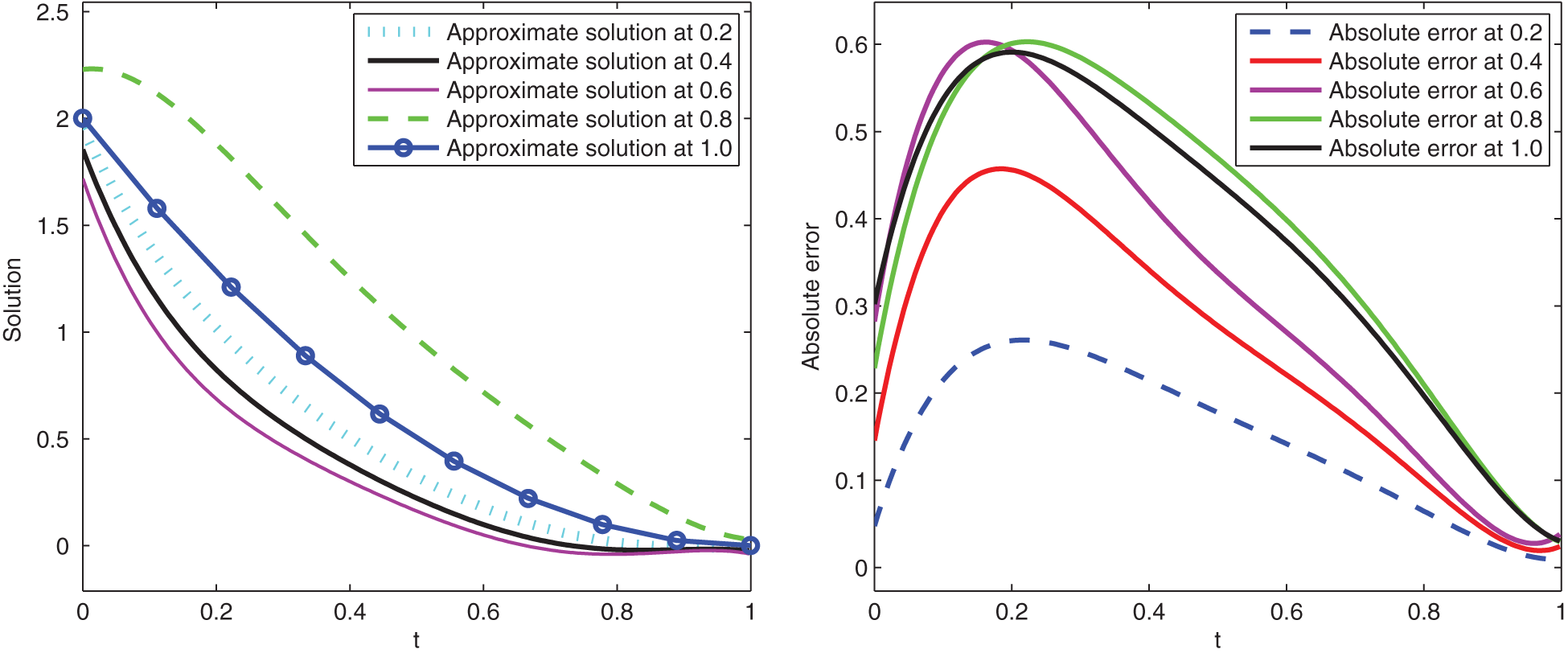
Figure 1: Graphical presentation of approximate solutions and absolute error of Example 1
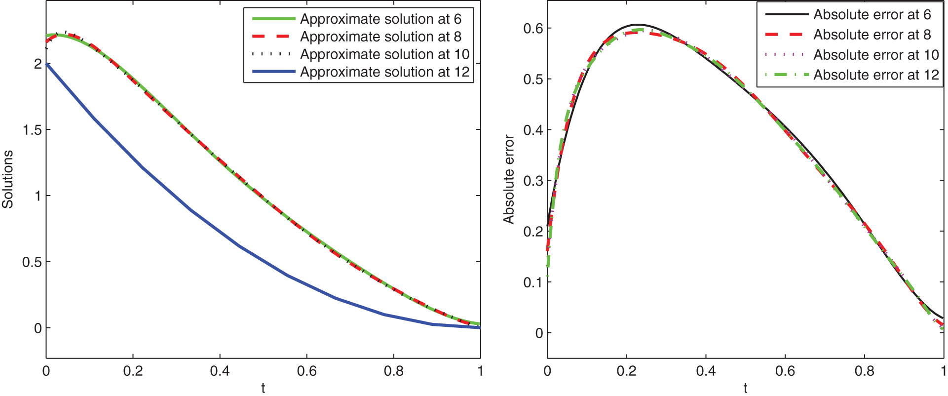
Figure 2: Graphical presentation of approximate solutions and absolute error of Example 1 at various scale level and at t = 0.75
Example 2. Consider another problem as
For
where the source function g is given as
Here, we give graphical presentation of approximate solution for various values of variable order at t and the corresponding absolute error using scale level equal to
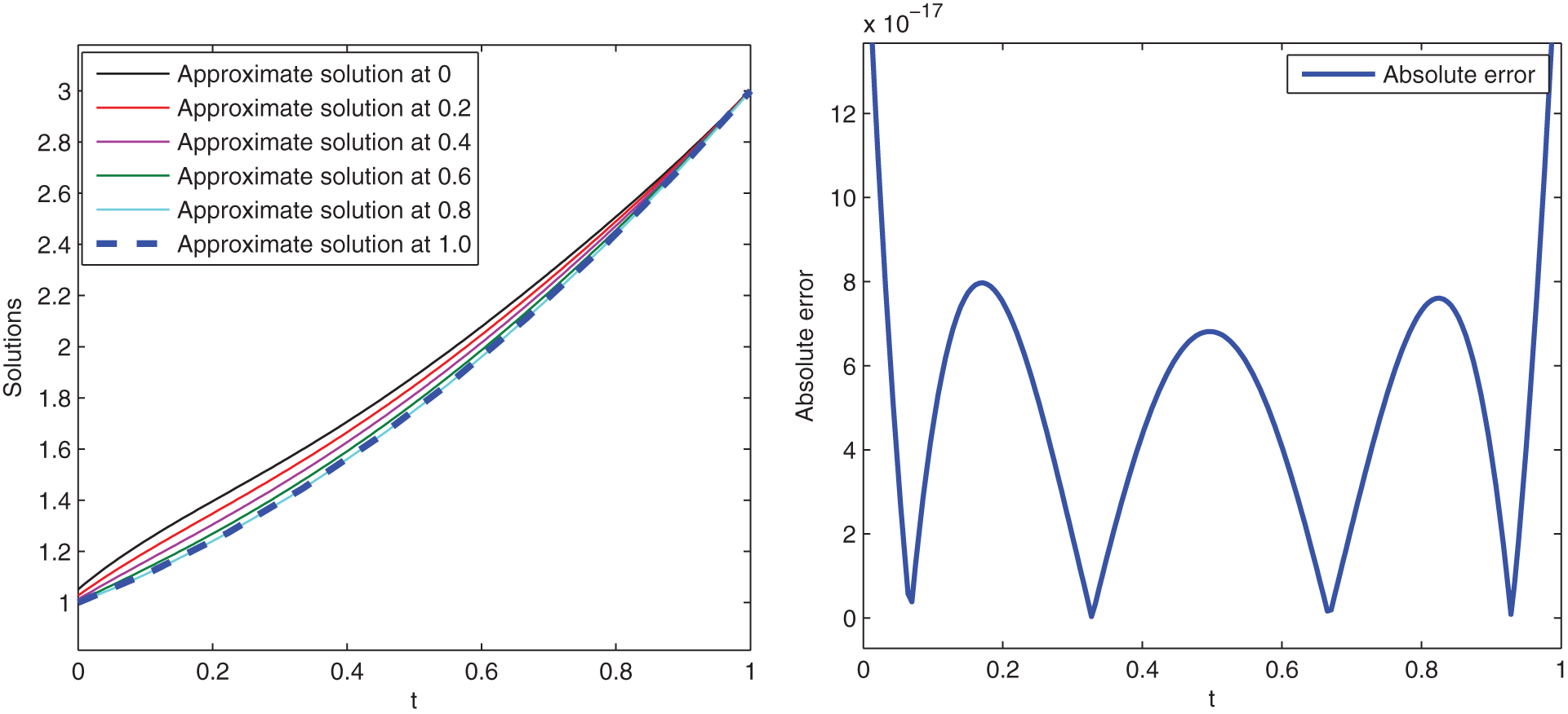
Figure 3: Graphical presentation of approximate solutions and absolute error of Example 2
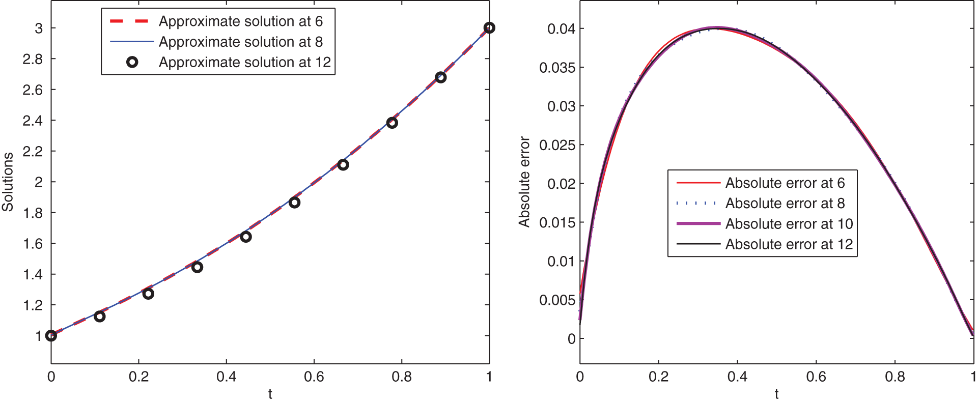
Figure 4: Graphical presentation of approximate solutions and absolute error of Example 2 at various scale level and at t = 0.75
4.2 Numerical Examples for Variable Order Boundary Value Problems
To demonstrate the second scheme for boundary value problems, we give some examples here.
Example 3. Consider the problem
For
Here, we give graphical presentation of approximate solution for various values of variable order at t and the corresponding absolute error using scale level equal to
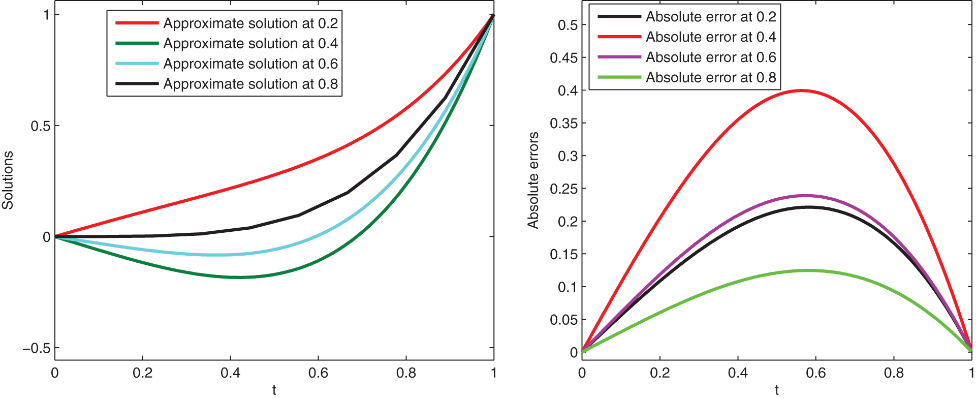
Figure 5: Graphical presentation of approximate solutions and absolute error of Example 3 at various values of t and scale level 6
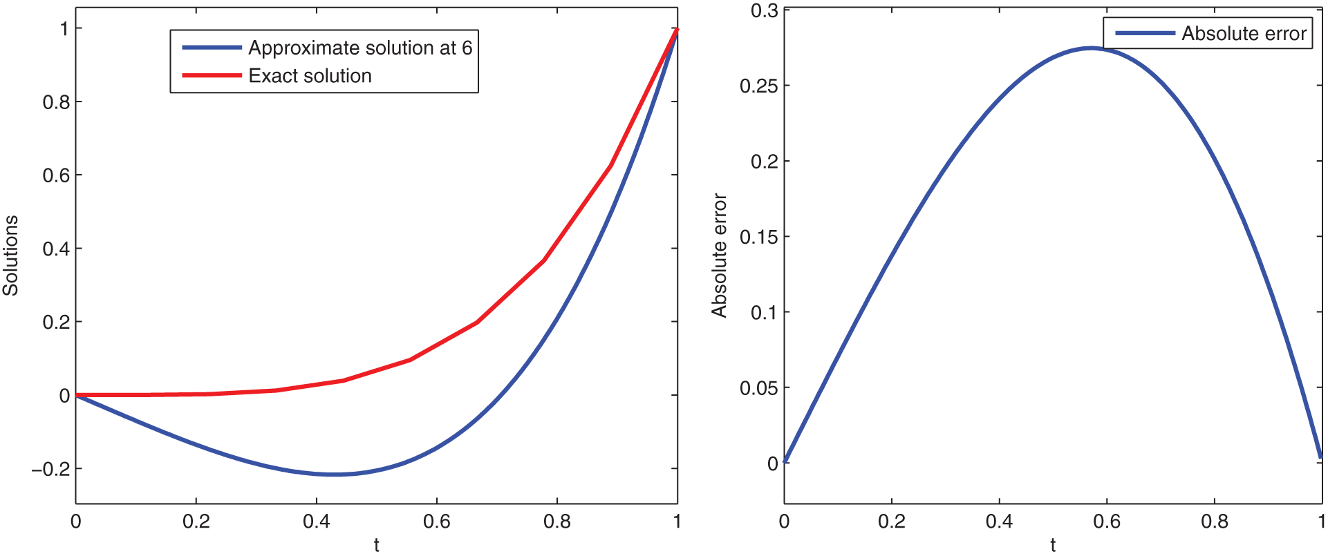
Figure 6: Graphical presentation of approximate solutions and absolute error of Example 3
Example 4. Consider the problem as
For
Here, we give graphical presentation of approximate solution for various values of variable order at t and the corresponding absolute error using scale level equal to
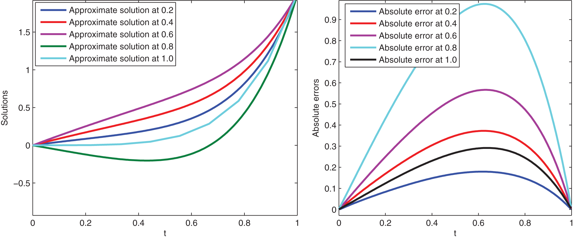
Figure 7: Graphical presentation of approximate solutions and absolute error of Example 4 at various values of t and scale level 6
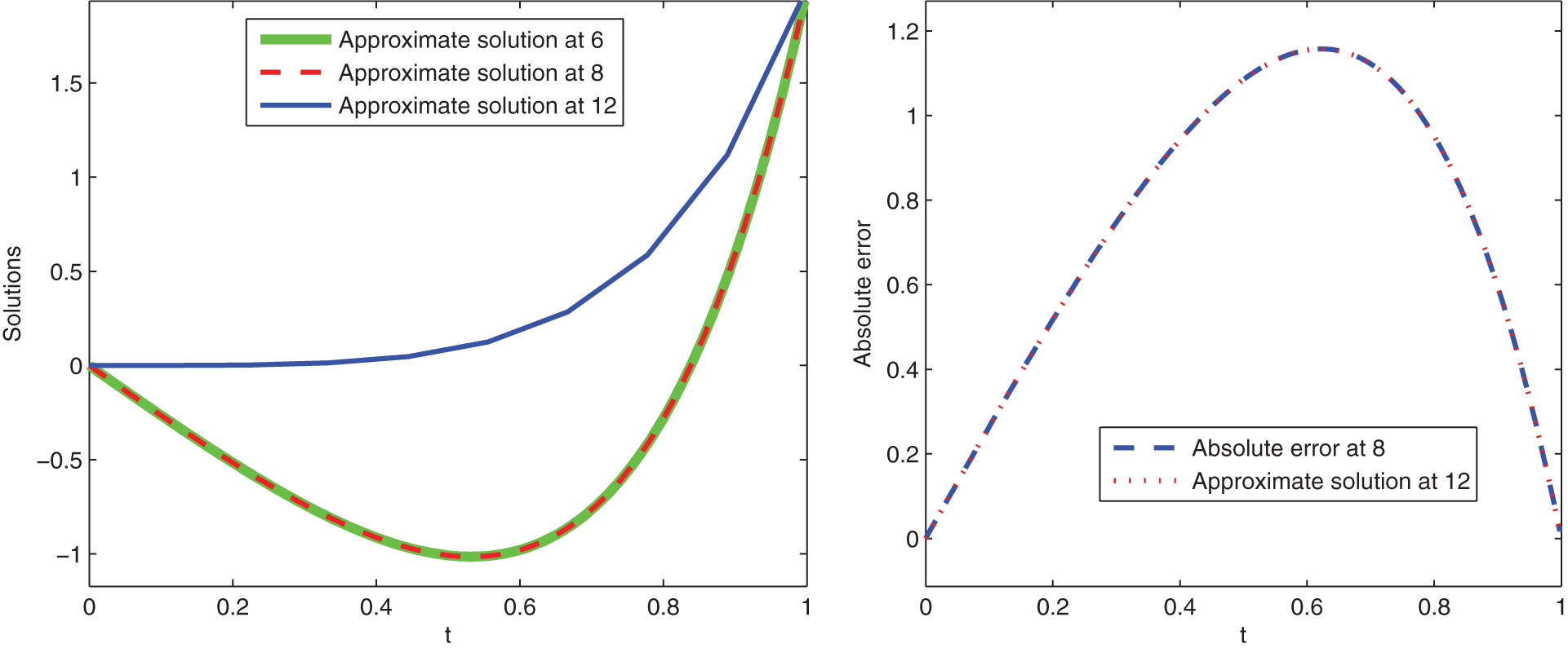
Figure 8: Graphical presentation of approximate solutions and absolute error of Example 4
In this research paper, various classes of variable order FDEs have been studied under boundary and initial conditions for numerical solutions. Properties of shifted Legendre polynomials have been used to develop operational matrices for fractional variable order derivative and integration. Based on these operational matrices, considered problems with initial/boundary conditions have been reduced to algebraic equations of the Sylvester type. By using mathematical softwares like Matlab, we have solved the obtained algebraic equation for the required numerical solution. In this regard, various examples have been solved based on the proposed method. We have omitted the collocations and sub-division of the time domain in small intervals. Also, the proposed spectral method has been proved stable. Moreover, some error analysis has been recorded which shows that the greater the scale level higher be the accuracy and vice versa. From our numerical experiments, we have observed that the accuracy of the proposed method is excellent and can be improved further by enlarging the scale level. Because of using a higher scale level, the efficiency of the proposed method can be improved very well. An absolute error has also been computed at different scale levels. We have also examined various problems using different fractional variable order to check the results. Hence, from numerical examples, we have concluded that the operational matrices method based on shifted Legendre polynomials can also be used as a powerful tool to handle different classes of variable order FDEs as well as integral equations for their numerical solutions.
Data Availability: The data used has been included within the paper.
Acknowledgement: This paper has been read and approved by all authors. Also authors Kamal Shah, Aziz Khan and Thabet Abdeljawad would like to thank Prince Sultan University for support through research lab TAS.
Funding Statement: Princess Nourah bint Abdurahman University Researchers Supporting Project No. (PNURSP2023R14), Princess Nourah bint Abdurahman University, Riyadh, Saudi Arabia.
Conflicts of Interest: The authors declare that they have no conflicts of interest to report regarding the present study.
REFERENCES
1. Miller, K. S., Ross B. (1993). An introduction to the fractional calculus and fractional differential equations. New York: Wiley. [Google Scholar]
2. Podlubny, I. (1998). Fractional differential equations. Amester Dam: Elsevier. [Google Scholar]
3. Oldham, K., Spanier, J. (1974). The fractional calculus theory and applications of differentiation and integration to arbitrary order. Amester Dam: Elsevier. [Google Scholar]
4. Ray, S. S., Bera, R. K. (2004). Solution of an extraordinary differential equation by adomian decomposition method. Journal of Applied Mathematics, 2004(4), 331–338. DOI 10.1155/S1110757X04311010. [Google Scholar] [CrossRef]
5. Chinnathambi, R., Rihan, F. A., Alsakaji, H. J. (2021). A fractional-order model with time delay for tuberculosis with endogenous reactivation and exogenous reinfections. Mathematical Methods in the Applied Sciences, 44(10), 8011–8025. DOI 10.1002/mma.5676. [Google Scholar] [CrossRef]
6. Hashim, I., Abdulaziz, O., Momani, S. (2009). Homotopy analysis method for fractional IVPs. Communications in Nonlinear Science and Numerical Simulation, 14(3), 674–684. DOI 10.1016/j.cnsns.2007.09.014. [Google Scholar] [CrossRef]
7. Rihan, F. A., Al-Mdallal, Q. M., AlSakaji, H. J., Hashish, A. (2019). A fractional-order epidemic model with time-delay and nonlinear incidence rate. Chaos, Solitons & Fractals, 126, 97–105. DOI 10.1016/j.chaos.2019.05.039. [Google Scholar] [CrossRef]
8. Canuto, C., Hussaini, M. Y., Quarteroni, A., Zang, T. A. (2007). Spectral methods: Fundamentals in single domains. Berlin/Heidelberg, Germany: Springer Science & Business Media. [Google Scholar]
9. Borhanifar, A., Sadri, K. (2015). Shifted jacobi collocation method based on operational matrix for solving the systems of fredholm and volterra integral equations. Mathematical and Computational Applications, 20(2), 76–93. DOI 10.3390/mca20010093. [Google Scholar] [CrossRef]
10. Saadatmandi, A., Dehghan, M. (2010). A new operational matrix for solving fractional-order differential equations. Computers & Mathematics with Applications, 59(3), 1326–1336. DOI 10.1016/j.camwa.2009.07.006. [Google Scholar] [CrossRef]
11. Khalil, H., Khan, R. A. (2014). A new method based on legendre polynomials for solutions of the fractional two-dimensional heat conduction equation. Computers & Mathematics with Applications, 67(10), 1938–1953. DOI 10.1016/j.camwa.2014.03.008. [Google Scholar] [CrossRef]
12. Rihan, F. A. (2013). Numerical modeling of fractional-order biological systems. Abstract and Applied Analysis, 2013. DOI 10.1155/2013/816803. [Google Scholar] [CrossRef]
13. Shah, K., Wang, J. (2019). A numerical scheme based on non-discretization of data for boundary value problems of fractional order differential equations. Revista de la Real Academia de Ciencias Exactas, Fsicas y Naturales. Serie A. Matemticas, 113(3), 2277–2294. DOI 10.1007/s13398-018-0616-7. [Google Scholar] [CrossRef]
14. Shah, K., Khalil, H., Khan, R. A. (2017). A generalized scheme based on shifted jacobi polynomials for numerical simulation of coupled systems of multi-term fractional-order partial differential equations. LMS Journal of Computation and Mathematics, 20(1), 11–29. DOI 10.1112/S146115701700002X. [Google Scholar] [CrossRef]
15. Mao, Z., Shen, J. (2017). Hermite spectral methods for fractional PDEs in unbounded domains. SIAM Journal on Scientific Computing, 39(5), A1928–A1950. DOI 10.1137/16M1097109. [Google Scholar] [CrossRef]
16. Khalil, H., Shah, K., Khan, R. A. (2017). Approximate solution of boundary value problems using shifted legendre polynomials. Applied and Computational Mathematics, 16(3), 269–285. [Google Scholar]
17. Rihan, F. A. (2010). Computational methods for delay parabolic and time-fractional partial differential equations. Numerical Methods for Partial Differential Equations, 26(6), 1556–1571. DOI 10.1002/num.20504. [Google Scholar] [CrossRef]
18. Chen, Y. M., Wei, Y. Q., Liu, D. Y., Yu, H. (2015). Numerical solution for a class of nonlinear variable order fractional differential equations with legendre wavelets. Applied Mathematics Letters, 46, 83–88. DOI 10.1016/j.aml.2015.02.010. [Google Scholar] [CrossRef]
19. Ganji, R. M., Jafari, H. (2019). Numerical solution of variable order integro-differential equations. Advanced Mathematical Models & Applications, 4(1), 64–69. [Google Scholar]
20. Moghaddam, B. P., Machado, J. A. T. (2017). Extended algorithms for approximating variable order fractional derivatives with applications. Journal of Scientific Computing, 71(3), 1351–1374. DOI 10.1007/s10915-016-0343-1. [Google Scholar] [CrossRef]
21. Patnaik, S., Hollkamp, J. P., Semperlotti, F. (2020). Applications of variable-order fractional operators: A review. Proceedings of the Royal Society A, 476(2234), 20190498. DOI 10.1098/rspa.2019.0498. [Google Scholar] [CrossRef]
22. Sun, H., Chang, A., Zhang, Y., Chen, W. (2019). A review on variable-order fractional differential equations: Mathematical foundations, physical models, numerical methods and applications. Fractional Calculus and Applied Analysis, 22(1), 27–59. DOI 10.1515/fca-2019-0003. [Google Scholar] [CrossRef]
23. Akgül, A., Baleanu, D. (2017). On solutions of variable-order fractional differential equations. International Journal of Optimization and Control: Theories & Applications, 7(1), 112–116. DOI 10.11121/ijocta.01.2017.00368. [Google Scholar] [CrossRef]
24. Gottlieb, D., Lustman, L., Tadmor, E. (1987). Stability analysis of spectral methods for hyperbolic initial-boundary value systems. SIAM Journal on Numerical Analysis, 24(2), 241–256. DOI 10.1137/0724020. [Google Scholar] [CrossRef]
25. Canuto, C., Hussaini, M. Y., Quarteroni, A., Zang, T. A. (1988). Theory of stability and convergence for spectral methods. In: Spectral methods in fluid dynamics, pp. 315–374. Berlin, Heidelberg: Springer. [Google Scholar]
26. Kendall, E. A. (2007). Numerical analysis. Scholarpedia, 2(8), 3163. DOI 10.4249/scholarpedia.3163. [Google Scholar] [CrossRef]
27. Bhrawy, A. H., Al-Shomrani, M. M. (2012). A shifted legendre spectral method for fractional-order multi-point boundary value problems. Advances in Difference Equations, 2012(1), 1–19. DOI 10.1186/1687-1847-2012-8. [Google Scholar] [CrossRef]
28. Adibi, H., Rismani, A. M. (2010). On using a modified legendre-spectral method for solving singular IVPs of Lane–Emden type. Computers & Mathematics with Applications, 60(7), 2126–2130. DOI 10.1016/j.camwa.2010.07.056. [Google Scholar] [CrossRef]
29. Dattoli, G., Ricci, P. E., Cesarano, C. (2001). A note on legendre polynomials. International Journal of Nonlinear Sciences and Numerical Simulation, 2(4), 365–370. DOI 10.1515/IJNSNS.2001.2.4.365. [Google Scholar] [CrossRef]
30. Dattoli, G., Germano, B., Martinelli, M. R., Ricci, P. E. (2011). A novel theory of legendre polynomials. Mathematical and Computer Modelling, 54(1–2), 80–87. DOI 10.1016/j.mcm.2011.01.037. [Google Scholar] [CrossRef]
31. Alrabaiah, H., Ahmad, I., Amin, R., Shah, K. (2021). A numerical method for fractional variable order pantograph differential equations based on haar wavelet. Engineering with Computers, 2021, 1–14. DOI 10.1007/s00366-020-01227-0. [Google Scholar] [CrossRef]
32. Heydari, M. H., Avazzadeh, Z. (2018). A new wavelet method for variable-order fractional optimal control problems. Asian Journal of Control, 20(5), 1804–1817. DOI 10.1002/asjc.1687. [Google Scholar] [CrossRef]
33. Hesthaven, J. S., Gottlieb, S., Gottlieb, D. (2007). Spectral methods for time-dependent problems, vol. 21. Cambridge: Cambridge University Press. [Google Scholar]
Cite This Article
 Copyright © 2023 The Author(s). Published by Tech Science Press.
This work is licensed under a Creative Commons Attribution 4.0 International License , which permits unrestricted use, distribution, and reproduction in any medium, provided the original work is properly cited.
 Downloads
 Citation Tools