
 Submit a Paper
 Propose a Special lssue
 Open Access
ARTICLE
A New Three-Parameter Inverse Weibull Distribution with Medical and Engineering Applications
1 Department of Mathematical Sciences, College of Science, Princess Nourah bint Abdulrahman University, Riyadh, 11671, Saudi Arabia
2 Department of Statistics, Faculty of Science, King Abdulaziz University, Jeddah, 21589, Saudi Arabia
3 Department of Mathematics, Faculty of Science, Al-Azhar University, Nasr City, 11884, Cairo, Egypt
4 Department of Statistics, Faculty of Commerce, Al-Azhar University, Nasr City, 11884, Cairo, Egypt
5 Department of Statistics, Faculty of Commerce, Zagazig University, Zagazig, 44519, Egypt
* Corresponding Authors: Mazen Nassar. Email: ,
(This article belongs to the Special Issue: New Trends in Statistical Computing and Data Science)
Computer Modeling in Engineering & Sciences 2023, 135(2), 1255-1274. https://doi.org/10.32604/cmes.2022.022623
Received 17 March 2022; Accepted 13 June 2022; Issue published 27 October 2022
 View Full Text
 Download PDF
Abstract
The objective of this article is to provide a novel extension of the conventional inverse Weibull distribution that adds an extra shape parameter to increase its flexibility. This addition is beneficial in a variety of fields, including reliability, economics, engineering, biomedical science, biological research, environmental studies, and finance. For modeling real data, several expanded classes of distributions have been established. The modified alpha power transformed approach is used to implement the new model. The data matches the new inverse Weibull distribution better than the inverse Weibull distribution and several other competing models. It appears to be a distribution designed to support decreasing or unimodal shaped distributions based on its parameters. Precise expressions for quantiles, moments, incomplete moments, moment generating function, characteristic generating function, and entropy expression are among the determined attributes of the new distribution. The point and interval estimates are studied using the maximum likelihood method. Simulation research is conducted to illustrate the correctness of the theoretical results. Three applications to medical and engineering data are utilized to illustrate the model’s flexibility.Keywords
Recently, many statistical distributions have been proposed by statisticians. The necessity to develop new distributions appear either due to practical investigations or theoretical concerns or both. Many applications in domains including dependability analysis, finance and risk modelling, insurance, and biological sciences, among others, have indicated in recent years that data sets that follow standard distributions are more often the exception than the usual. Because modified distributions are necessary, significant progress has been made in the modification of several classic distributions and their efficient utilization to challenges in these fields. Lately, specifically since 1980, the direction of statisticians to develop new distributions is on adding parameter(s) to some existing distributions or integrating classical distributions, see Lee et al. [1]. This addition of parameter(s) has been demonstrated valuable in analysing tail properties and also for enhancing the goodness of fit of the family under consideration. For more details about the methods of adding parameters, one can refer to Mudholkar et al. [2], Marshall et al. [3] and Mahdavi et al. [4].
The inverse-Weibull (IW) distribution has many vital applications in life testing and reliability studies. The IW distribution bears some other names like Fréchet distribution. The IW distribution is viewed as reciprocal to the usual Weibull distribution, see Drapella [5] and Mudholkar et al. [6], it is used to describe the degradation of mechanical components in diesel engines, such as the crankshaft and pistons, see Keller et al. [7]. Several academics proposed several modified variations of the IW distribution to increase its flexibility. Khan [8] looked at the beta IW distribution, for example. The generalized IW distribution was proposed by de Gusmao et al. [9], the modified IW distribution was proposed by Khan et al. [10], the Kumaraswamy generalized IW distribution was proposed by Oluyede et al. [11], and the Kumaraswamy modified IW distribution was proposed by Aryal et al. [12]. In addition, Okasha et al. [13] suggested the Marshall-Olkin IW distribution, Basheer [14] proposed the alpha power IW distribution, Dey et al. [15] discussed the logarithmic transformed IW distribution, and Afify et al. [16] suggested the logarithmic transformed IW distribution.
Assume that X is a random variable follows IW distribution with
The cumulative distribution function (CDF) of Eq. (1) is
See Johnson et al. [17] for further information on the IW distribution. In this study, we offer a new three-parameter IW distribution utilizing the same idea proposed by Alotaibi et al. [18]. The modified alpha power transformed IW (MAPTIW) distribution is the name given to the new distribution. Two shape parameters and one scale parameter are included. It includes some lifetime distributions, such as IW, inverted exponential and inverse Rayleigh distributions. Recently, The alpha power transformation approach was used by Alotaibi et al. [18] to suggest a new method for adding a new shape parameter to a baseline distribution. Modified alpha power transformation (MAPT) was the name given to the approach they proposed. The CDF and PDF of MAPT method are expressed as
and
where
The remainder of this article is structured as follows. The MAPTIW distribution is introduced and its mixed representation is derived in Section 2. In Section 3, we will look at some of the MAPTIW’s most important characteristics. Section 4 shows how to estimate unknown parameters using maximum likelihood estimation. We present the simulation results in Section 5 to show how well the estimations performed. Three real-life data sets are used to assess the importance of the MAPTIW distribution in Section 6. Section 7 presents the conclusion.
We may define the CDF of the MAPTIW distribution in the following form by inserting the CDF of the IW distribution obtained by Eq. (2) into the CDF of the MAPT generator given by Eq. (3)
The PDF that corresponds to the CDF in Eq. (5) can be expressed as follows:
MAPTIW distribution has the following special sub-models. If
and
respectively. Henceforth, we will use X to refer to the random variable that possesses the PDF in Eq. (6).
The various plots of the PDF of the MAPTIW distribution with
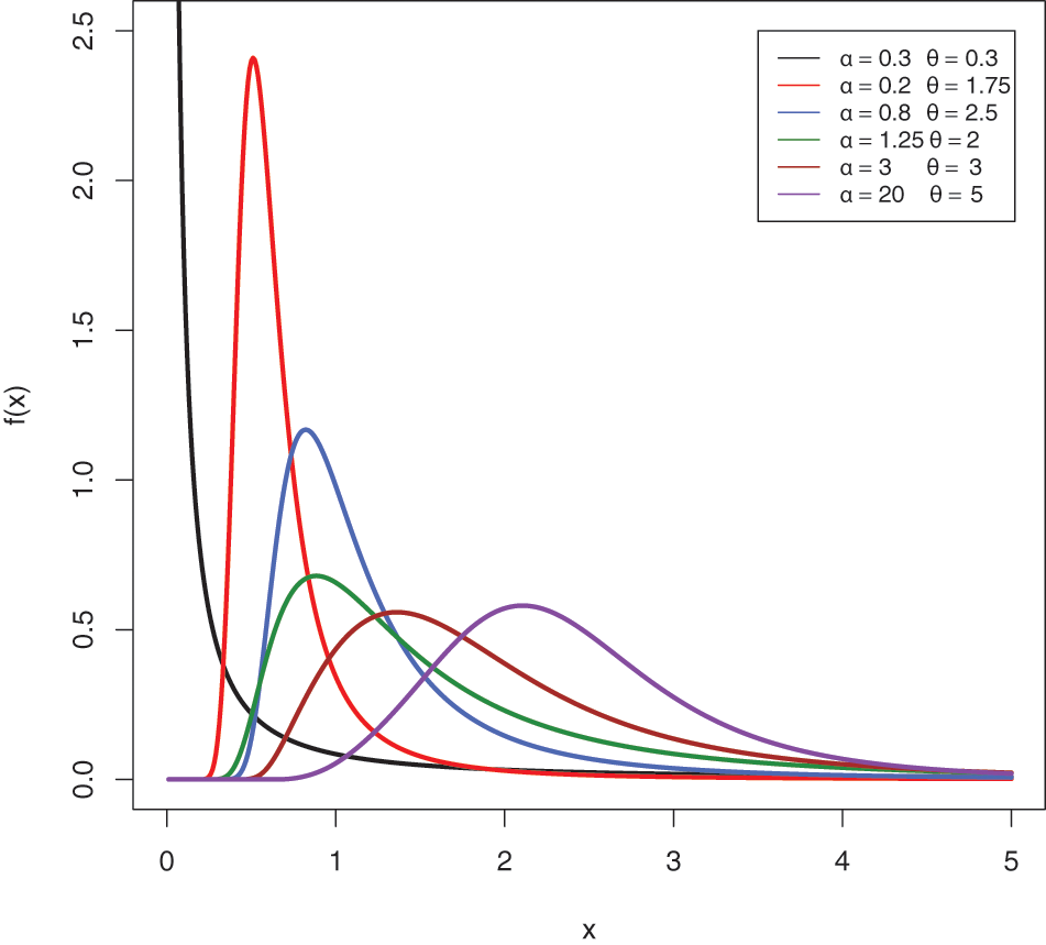
Figure 1: MAPTIW PDF plots
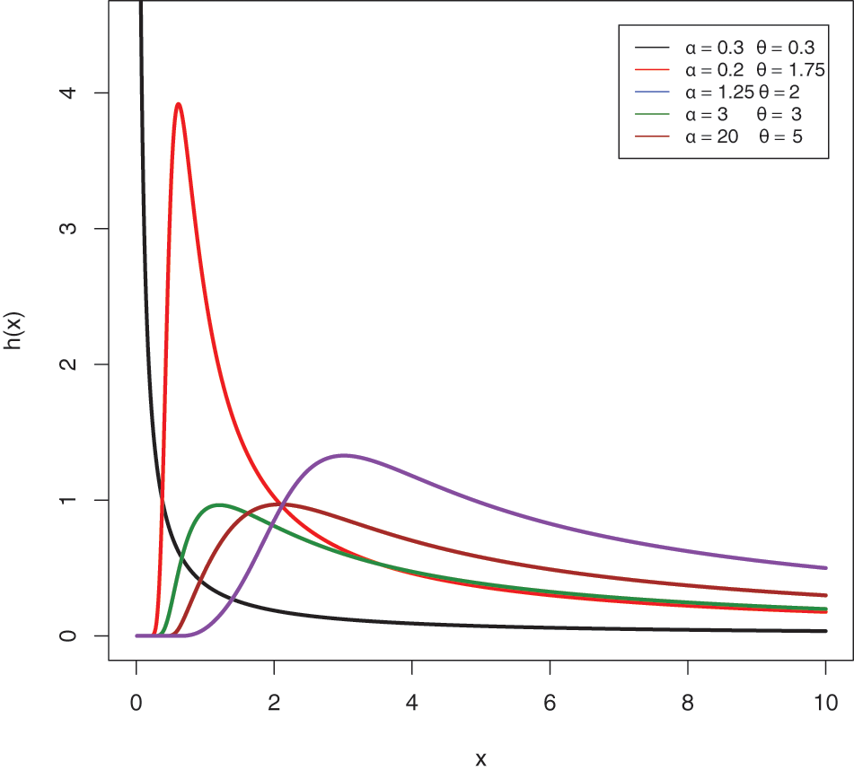
Figure 2: HRF plots for the MAPTIW distribution
The PDF in Eq. (6) might be used to obtain various statistical characteristics of the MAPTIW distribution. Finding the PDF’s mixture structure in Eq. (5) is a simple method. Observe the power series below:
where y is a variable and
where y is a variable,
When Eqs. (9) and (10) are applied to the PDF in Eq. (6), the following is a suitable linear representation for the PDF
where
On the other hand, the expansion of the CDF in Eq. (5) may be provided as by integrating Eq. (11) as
Hence
3 MAPTIW Distribution’s Properties
The quantile function, moments and stress-strength parameter are some of the properties of the MAPTIW distribution that we derive in this part.
The quantile function for the MAPTIW distribution may be calculated as follows using Eq. (5):
One can employ Eq. (13) to simulate the random variable X by taking
Moments play an essential part in statistics. Numerous vital aspects of any statistical distribution can be explored via moments. For the MAPTIW distribution, the
where
and
The following formulae can also be used to obtain the variance (var), skewness (Sk), and kurtosis (Ku):
and
where
Prop 3.1. If
where
Prop 3.2. If
and
Prop 3.3. If
Prop 3.4. If
where
3.3 Entropies of MAPTIW Distribution
Entropy is used to measure uncertainty. It recreates a vital role in the area of engineering, probability, statistics, information theory and financial analysis. For example, Gençay et al. [19] delivered a relative analysis of the stock market during the 1987 and 2008 financial crises. Rashidi et al. [20] examined and simulated the heat transfer flow employing entropy generation in solar still. The Rényi entropy (RE) for the MAPTIW distribution may be calculated using Eq. (6) as follows:
The Shannon entropy can also be calculated as
Let
The beta function is represented as
where
Using Eq. (17), we can derive the properties of
3.5 Moments of Residual Life and Reversed Failure Rate Function
The mean residual lifetime has been studied by engineers and survival analysts. Given a feature or a system is of age
Using Eqs. (5) and (6), and the binomial expansion of
The mean residual lifetime can be obtained from the last equation by setting
Based on Eqs. (5), (6) and using the binomial expansion of
Let
Case one:
Using the series expansion in Eq. (10), it follows:
Using the series expansion in Eq. (9), we can obtain
where
and
Case two:
Using the series expansion in Eq. (10), we have
Using the series expansion in Eq. (9), we can obtain
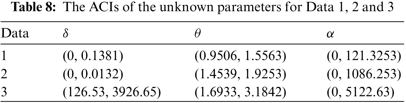
In this section, we consider the maximum likelihood approach to estimate the unknown parameters of the MAPTIW distribution. Furthermore, the approximate confidence intervals (ACIs) of the unknown parameters are acquired.
4.1 Maximum Likelihood Estimation
Given a random sample of size n taken from the MAPTIW distribution with PDF given by Eq. (6), we can express the log-likelihood function as
The maximum likelihood estimates (MLEs) denoted by
and
where
and
To get the MLEs of
where
and
where
and
Therefore, the
where
In this part, we use a simulation with variable sample sizes n and various values of the parameters
1. Establish the sample size and parameter initial values.
2. Create a random sample of size n from the MAPTIW distribution using Eq. (13).
3. Compute the MLEs of
4. Compute the MSEs of
5. Get the CLs of
6. Redo Steps 2–5, 1000 times.
7. Determine the average values of estimates (AEs), MSEs, and CLs as follows:


In this part, we illustrate the MAPTIW distribution’s flexibility by using three real data sets. The MAPTIW distribution is compared to other models such as, alpha power inverse Lomax (APILo) distribution by ZeinEldin et al. [21], inverse Lomax (ILo) distribution, alpha power inverse Weibull (APIW) distribution by Basheer [14], alpha power inverse Lindley (APILi) distribution by Dey et al. [22] and Weibull (We) distribution. Table 4 displays the PDFs of these distributions.

The first data (Data 1) describes the mortality rates due to the COVID-19 pandemic in the United Kingdom for 76 days, from 15 April to 30 June 2020. The data is originally investigated by Mubarak et al. [23]. The entire data set is as follows: 0.0587, 0.0863, 0.1165, 0.1247, 0.1277, 0.1303, 0.1652, 0.2079, 0.2395, 0.2751, 0.2845, 0.2992, 0.3188, 0.3317, 0.3446, 0.3553, 0.3622, 0.3926, 0.3926, 0.4110, 0.4633, 0.4690, 0.4954, 0.5139, 0.5696, 0.5837, 0.6197, 0.6365, 0.7096, 0.7193, 0.7444, 0.8590, 1.0438, 1.0602, 1.1305, 1.1468, 1.1533, 1.2260, 1.2707, 1.3423, 1.4149, 1.5709, 1.6017, 1.6083, 1.6324, 1.6998, 1.8164, 1.8392, 1.8721, 1.9844, 2.1360, 2.3987, 2.4153, 2.5225, 2.7087, 2.7946, 3.3609, 3.3715, 3.7840, 3.9042, 4.1969, 4.3451, 4.4627, 4.6477, 5.3664, 5.4500, 5.7522, 6.4241, 7.0657, 7.4456, 8.2307, 9.6315, 10.187, 11.1429, 11.2019, 11.4584.
The second data set (Data 2) describes the remission times (in months) of a random sample of 128 bladder cancer patients studied by Lee et al. [24] and recently investigated by Al-Zahrani et al. [25–27]. The complete data set of is: 0.08, 2.09, 3.48, 4.87, 6.94, 8.66, 13.11, 23.63, 0.20, 2.23, 3.52, 4.98, 6.97, 9.02, 13.29, 0.40, 2.26, 3.57, 5.06, 7.09, 9.22, 13.80, 25.74, 0.50, 2.46, 3.64, 5.09, 7.26, 9.47, 14.24, 25.82, 0.51, 2.54, 3.70, 5.17, 7.28, 9.74, 14.76, 26.31, 0.81, 2.62, 3.82, 5.32, 7.32, 10.06, 14.77, 32.15, 2.64, 3.88, 5.32, 7.39, 10.34, 14.83, 34.26, 0.90, 2.69, 4.18, 5.34, 7.59, 10.66, 15.96, 36.66, 1.05, 2.69, 4.23, 5.41, 7.62, 10.75, 16.62, 43.01, 1.19, 2.75, 4.26, 5.41, 7.63, 17.12, 46.12, 1.26, 2.83, 4.33, 5.49, 7.66, 11.25, 17.14, 79.05, 1.35, 2.87, 5.62, 7.87, 11.64, 17.36, 1.40, 3.02, 4.34, 5.71, 7.93, 11.79, 18.10, 1.46, 4.40, 5.85, 8.26, 11.98, 19.13, 1.76, 3.25, 4.50, 6.25, 8.37, 12.02, 2.02, 3.31, 4.51, 6.54, 8.53, 12.03, 20.28, 2.02, 3.36, 6.76, 12.07, 21.73, 2.07, 3.36, 6.93, 8.65, 12.63, 22.69.
The third data set (Data 3) consists of the times of breakdown of a sample of 25 devices at
Before studying these data sets, we foremost scheme the corresponding TTT plots. Fig. 3 displays the TTT plots of these data. It indicates that Data 1 has a decreasing failure rate function, while the TTT plots for Data 2 and 3 reveal an upside-down bathtub failure rate function. Therefore, we can infer that the MAPTIW distribution is reasonable to model these data sets. The MLEs and their standard errors (SEs) of the MAPTIW distribution and some other competitive distributions are displayed in Tables 5, 6 and 7 for Data 1, 2 and 3, respectively. In addition, some goodness of fit statistics, namely, Akaike information criterion (AIC), consistent Akaike information criterion (CAIC), Bayesian information criterion (BIC), Hannan-Quinn information criterion (HQIC) statistics, Anderson-Darling (A), Cramér-Von Mises
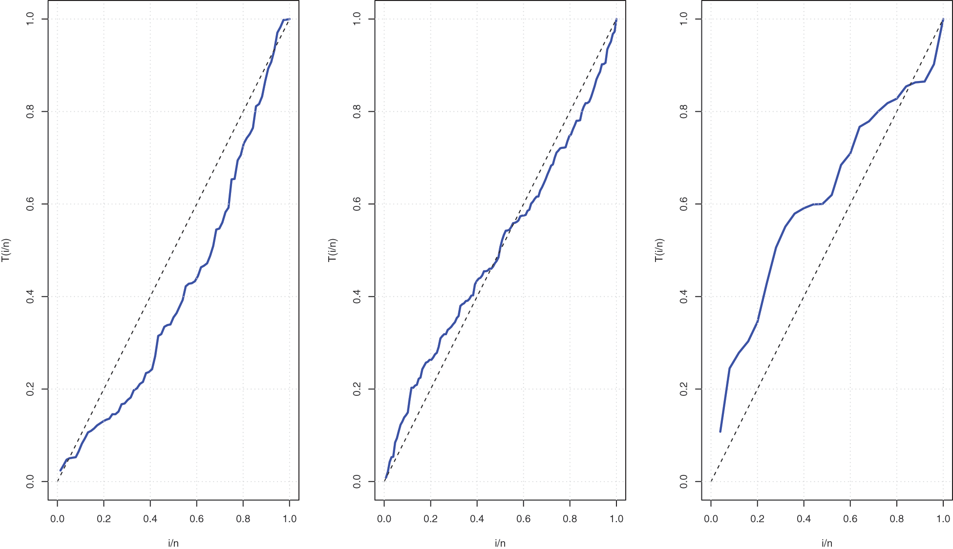
Figure 3: TTT Plots for Data 1 (left) and Data 2 (middle) and Data 3 (right)

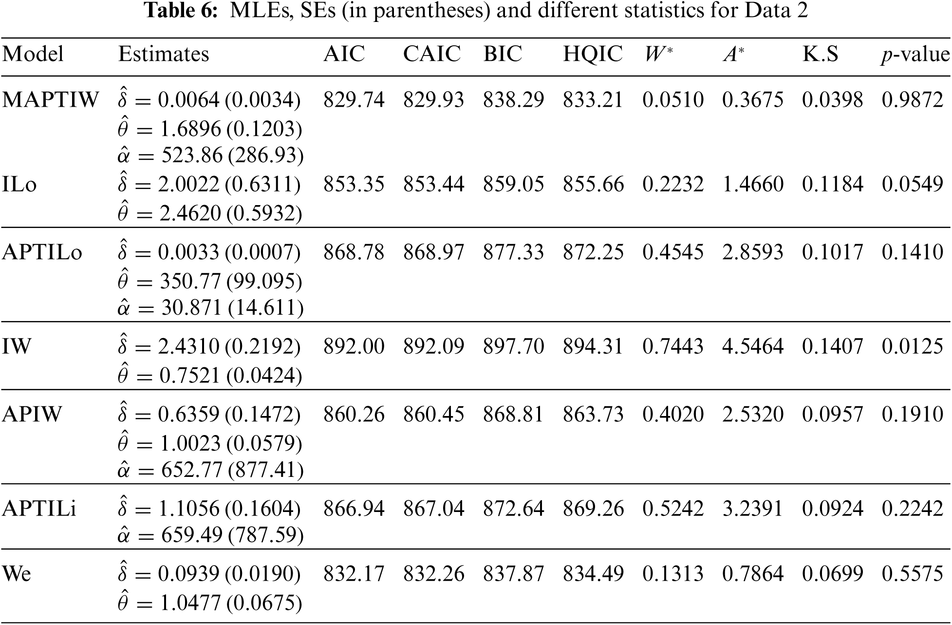
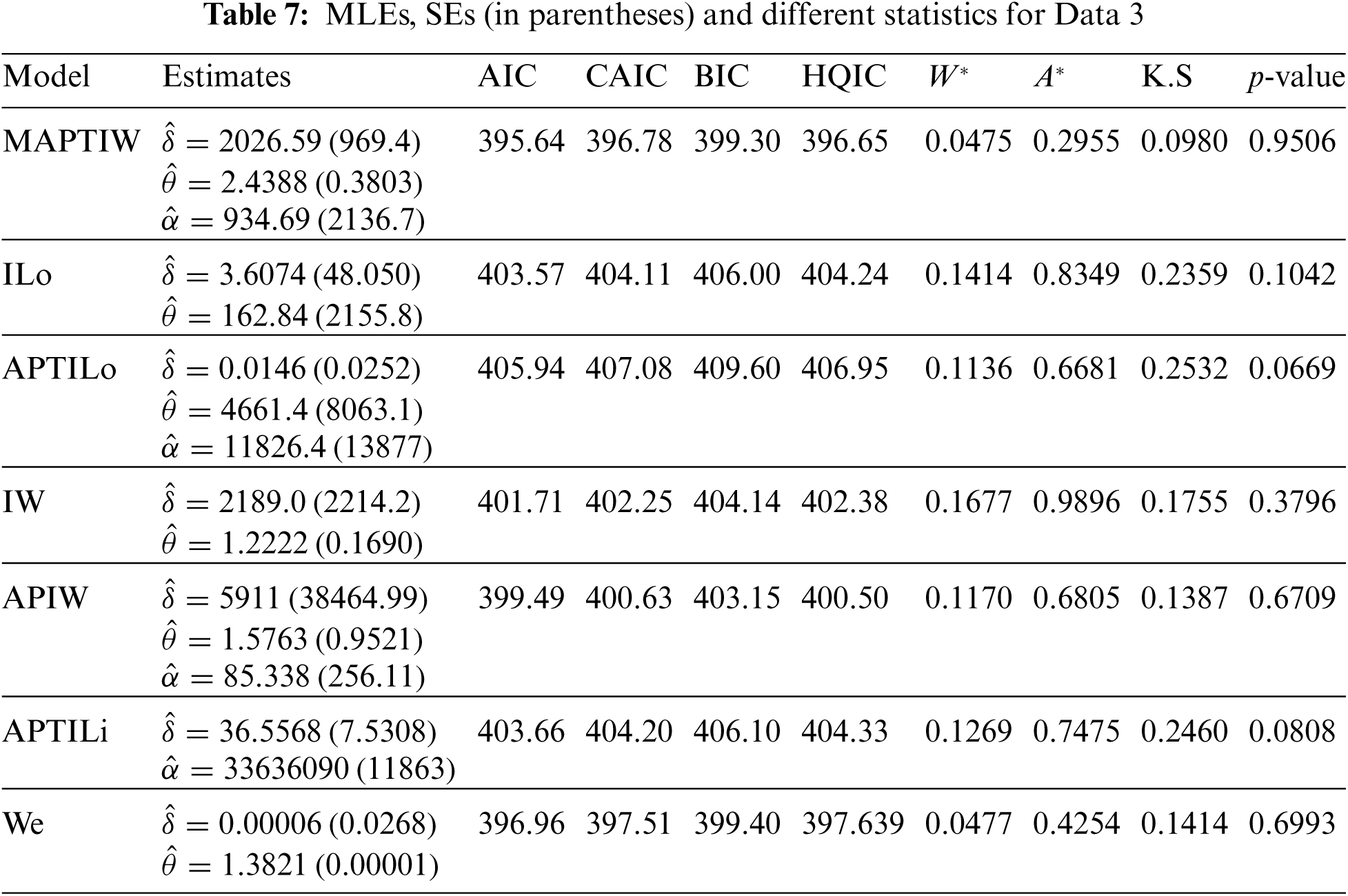

Figure 4: Plots of the fitted functions for the MAPTIW distribution and PP plot for Data 1

Figure 5: Plots of the fitted functions for the MAPTIW distribution and PP plot for Data 2

Figure 6: Plots of the fitted functions for the MAPTIW distribution and PP plot for Data 3
As a new extension of the inverse Weibull model, we introduced a new three-parameter inverse Weibull distribution. Additionally, numerous theoretical properties of the distribution were explored in order to develop a more flexible model that includes the decreasing and unimodal shape for the hazard rate function. We described the method of maximum likelihood for estimating the parameters of the suggested distribution. A simulation study is also used to investigate the asymptotic behaviour of the maximum likelihood estimators. The model’s efficiency is demonstrated using three real data sets to show its applicability in real life. The proposed distribution is a better distributional model for fitting such data sets than many of its related models, as well as several newly produced distributions, using various information measures.
Acknowledgement: The authors convey their sincere appreciation to the reviewers and the editors for making some valuable suggestions and comments. The authors extend their appreciations to Princess Nourah bint Abdulrahman University Researchers Supporting Project No. (PNURSP2022R50), Princess Nourah bint Abdulrahman University, Riyadh, Saudi Arabia.
Funding Statement: This research was funded by Princess Nourah bint Abdulrahman University Researchers Supporting Project No. (PNURSP2022R50), Princess Nourah bint Abdulrahman University, Riyadh, Saudi Arabia.
Conflicts of Interest: The authors declare that they have no conflicts of interest to report regarding the present study.
References
1. Lee, C., Famoye, F., Alzaatreh, A. (2013). Methods for generating families of univariate continuous distributions in the recent decades. WIREs, 5, 219–238. DOI 10.1002/wics.1255. [Google Scholar] [CrossRef]
2. Mudholkar, G. S., Srivastava, D. K. (1993). Exponentiated weibull family for analyzing bathtub failure-rate data. IEEE Transactions on Reliability, 42, 299–302. DOI 10.1109/24.229504. [Google Scholar] [CrossRef]
3. Marshall, A. W., Olkin, I. (1997). A new method for adding a parameter to a family of distributions with application to the exponential and weibull families. Biometrika, 84, 641–652. DOI 10.1093/biomet/84.3.641. [Google Scholar] [CrossRef]
4. Mahdavi, A., Kundu, D. (2017). A new method for generating distributions with an application to exponential distribution. Communications in Statistics–Theory and Methods, 46(13), 6543–6557. DOI 10.1080/03610926.2015.1130839. [Google Scholar] [CrossRef]
5. Drapella, A. (1993). Complementary weibull distribution: Unknown or just forgotten. Quality and Reliability Engineering International, 9, 383–385. DOI 10.1002/(ISSN)1099-1638. [Google Scholar] [CrossRef]
6. Mudholkar, G. S., Kollia, G. D. (1994). Generalized weibull family: A structural analysis. Communications in Statistics-Theory and Methods, 23, 1149–1171. DOI 10.1080/03610929408831309. [Google Scholar] [CrossRef]
7. Keller, A. Z., Kamath, A. R. (1982). Reliability analysis of CNC machine tools. Reliability Engineering, 3, 449–473. DOI 10.1016/0143-8174(82)90036-1. [Google Scholar] [CrossRef]
8. Khan, M. S. (2010). The beta inverse weibull distribution. International Transactions in Mathematical Sciences and Computer, 3, 113–119. [Google Scholar]
9. de Gusmao, F. R., Ortega, E. M., Cordeiro, G. M. (2011). The generalized inverse Weibull distribution. Statistical Papers, 52, 591–619. DOI 10.1007/s00362-009-0271-3. [Google Scholar] [CrossRef]
10. Khan, M. S., King, R. (2012). Modifieed inverse Weibull distribution. Journal of Statistics Applications & Probability, 1, 115–132. DOI 10.12785/jsap/010204. [Google Scholar] [CrossRef]
11. Oluyede, B. O., Yang, T. (2014). Generalizations of the inverse weibull and related distributions with applications. Electronic Journal of Applied Statistical Analysis, 7, 94–116. [Google Scholar]
12. Aryal, G., Elbatal, I. (2015). Kumaraswamy modified inverse weibull distribution. Applied Mathematics & Information Sciences, 9, 651–660. [Google Scholar]
13. Okasha, H. M., El-Baz, A. H., Tarabia, A. M. K., Basheer, A. M. (2017). Extended inverse weibull distribution with reliability application. Journal of the Egyptian Mathematical Society, 25, 343–349. DOI 10.1016/j.joems.2017.02.006. [Google Scholar] [CrossRef]
14. Basheer, A. M. (2019). Alpha power inverseWeibull distribution with reliability application. Journal of Taibah University for Science, 13, 423–432. DOI 10.1080/16583655.2019.1588488. [Google Scholar] [CrossRef]
15. Dey, S., Nassar, M., Kumar, D., Alaboud, F. (2019). Logarithm transformed fréchet distribution: Properties and estimation. Austrian Journal of Statistics, 48(1), 70–93. DOI 10.17713/ajs.v48i1.634. [Google Scholar] [CrossRef]
16. Afify, A. Z., Ahmed, S., Nassar, M. (2021). A new inverse weibull distribution: Properties, classical and Bayesian estimation with applications. Kuwait Journal of Science, 48(3), 1–10. [Google Scholar]
17. Johnson, N. L., Kotz, S., Balakrishnan, N. (1995). In: Continuous univariate distributions, 2nd ed., vol. 2. New York, NY, USA: Wiley. [Google Scholar]
18. Alotaibi, R., Okasha, H., Rezk, H., Nassar, M. (2021). A new weighted version of alpha power transformation method: Properties and applications to COVID-19 and software reliability data. Physica Scripta, 96, 125–221. DOI 10.1088/1402-4896/ac2658. [Google Scholar] [CrossRef]
19. Genç, R., Gradojevic, N. (2017). The tale of two financial crises: An entropic perspective. Entropy, 19(6), 244. DOI 10.3390/e19060244. [Google Scholar] [CrossRef]
20. Rashidi, S., Akar, S., Bovand, M., Ellahi, R. (2018). Volume of fluid model to simulate the nanofluid flow and entropy generation in a single slope solar still. Renewable Energy, 115, 400–410. DOI 10.1016/j.renene.2017.08.059. [Google Scholar] [CrossRef]
21. ZeinEldin, R. A., Ahsan ul Haq, M., Hashmi, S., Elsehety, M. (2020). Alpha power transformed inverse lomax distribution with different methods of estimation and applications. Complexity, DOI 10.1155/2020/1860813. [Google Scholar] [CrossRef]
22. Dey, S., Nassar, M., Kumar, D. (2019). Alpha power transformed inverse lindley distribution: A distribution with an upside-down bathtub-shaped hazard function. Journal of Computational and Applied Mathematics, 348, 130–145. DOI 10.1016/j.cam.2018.03.037. [Google Scholar] [CrossRef]
23. Mubarak, A. E., Al-Metwally, E. (2021). A New Extension Exponential Distribution with Applications of COVID-19 Data. https://jsst.journals.ekb.eg. [Google Scholar]
24. Lee, E. T., Wang, J. (2003). Statistical methods for survival data analysis. New Jersey, USA: John Wiley & Sons. [Google Scholar]
25. Al-Zahrani, B., Sagor, H. (2015). Statistical analysis of the lomax-logarithmic distribution. Journal of Statistical Computation and Simulation, 85(9), 1883–1901. DOI 10.1080/00949655.2014.907800. [Google Scholar] [CrossRef]
26. Shakhatreh, M. K. (2018). A new three-parameter extension of the log-logistic distribution with applications to survival data. Communications in Statistics–Theory and Methods, 47(21), 5205–5226. DOI 10.1080/03610926.2017.1388399. [Google Scholar] [CrossRef]
27. Klakattawi, H. S. (2022). Survival analysis of cancer patients using a new extended weibull distribution. PLoS One, 17(2), e0264229. DOI 10.1371/journal.pone.0264229. [Google Scholar] [CrossRef]
28. Pham, H. (2003). Accelerated life testing. In: Hoang Pham (Ed.Handbook of reliability engineering, vol. 1. London: Springer. [Google Scholar]
Cite This Article
 Copyright © 2023 The Author(s). Published by Tech Science Press.
This work is licensed under a Creative Commons Attribution 4.0 International License , which permits unrestricted use, distribution, and reproduction in any medium, provided the original work is properly cited.
 Downloads
 Citation Tools