Panel Acoustic Contribution Analysis in Automotive Acoustics Using Discontinuous Isogeometric Boundary Element Method

1  Introduction

In the noise, vibration and harshness (NVH) field of automotive engineering, the panel acoustic contribution analysis (PACA) [1,2] is a popular technique to identify the critical panels that contribute most to the sound pressure at an interior point of interest, for example, the position of driver’s ear. The automotive body panels can be ranked according to their contribution to the sound pressure by using PACA, which will guide the structure acoustic optimization to improve the NVH performance.

The idea of PACA was initially established by a commercial software company to identify the relative acoustic contribution of structure panels to the sound pressure at points of interest [3,4]. The key process of PACA is to obtain the sound pressure and the velocity at the panel surface; it is commonly implemented either by experimental or numerical methods. The experiment-based methods, such as transfer path analysis (TPA) [5,6] and reciprocally measured transfer function (RMTF) [7,8], include at least two experiment steps. The first step is to build the transfer function between the excitation and the sound response at the observing point, and the second step is to obtain the response at the same point based on the excitations measured. These approaches are remarkably time and effort-consuming in automotive engineering problems. Another implementation of PACA is its combination with traditional numerical methods, for example, the finite element method (FEM) [9] and the boundary element method (BEM) [10]. However, such a combination benefits the accuracy of the numerical methods, but also inherits the drawback at the same time. For example, the mesh generation is time-consuming in automotive acoustics using FEM, given that the discretization in the entire acoustic field is required. The computing cost of PACA combined with BEM is also high because the final matrix equation is fully populated and unsymmetrical. Moreover, the singularity should be dealt with specific schemes. Thus, the demands are high on developing a more accurate and efficient method to identify the critical panels in the automotive NVH engineering.

Isogeometric analysis (IGA) has developed rapidly since it was proposed by Hughes to bridge the gap between the design model and the analysis model [11]. The combination of IGA and BEM brings new research prospects in the acoustic research area [12,13]. In isogeometric boundary element method (IGABEM), non-uniform rational B-splines (NURBS) are considered basis functions to express the problem geometry as well as the solution variables [14–16], thereby simplifying the meshing process and improving the accuracy. Thus far, the research on IGABEM is mostly restrained in the application of continuous elements and single-type boundary condition problems [17]. However, in most engineering issues, the structure geometry is complex, where the normal vector on the unsmooth boundary is discontinuous. Moreover, the boundary conditions of these realistic problems are mostly mixed types. For example, in the interior noise calculation of the car passenger compartment, the properties of the lining material and the window glass are evidently different. In such a situation, discretizing the geometry or variables using continuous elements causes extremely large calculation errors [18–20]. This condition is the corner problem in BEM, which must be dealt with appropriate strategies. Earlier work [21] by the authors has proposed a discontinuous IGABEM that introduces the “double nodes” technique to IGABEM, presenting a more efficient numerical approximation in the circumstance of corner problems, where the geometry and primary variable exhibit large gradients or discontinuities. In the previous work, the discontinuous IGABEM has shown an evident advantage over the continuous IGABEM and BEM in terms of accuracy and converge speed of a real car compartment radiation noise problem.

This study is a follow-up work to investigate the combination of PACA and discontinuous IGABEM in addressing automotive acoustic problems. To the best of the authors’ knowledge, published studies on these concepts are limited. Thus, we attempt to fill this void by developing an easily applicable and efficient numerical method to analyze the relative acoustic contributions from automotive body panels.

The remainder of the paper is structured as follows. First, an introduction to the discontinuous IGABEM is given in Section 2. Section 3 presents the idea of PACA and the implementation based on discontinuous IGABEM. Two numerical examples are illustrated in Section 4 to verify the accuracy and efficiency of the proposed scheme, including a car passenger compartment subjected to realistic boundary conditions. An experiment is conducted to validate the proposed method in Section 5. Finally, conclusions are drawn in Section 6.

2  Discontinuous Isogeometric Boundary Element Formulation

2.1 NURBS

A brief introduction of B-splines and NURBS is presented in this subsection. NURBS are built from B-splines and the construction of B-Splines starts from the concept of knot vector [22,23]. A knot vector Ξ in 1D is a series of non-decreasing real numbers, as follows:

Ξ={ξ1,…,ξi,…,ξl+p+1},ξi∈R(1)

where i=1,2,…,l+p+1, l is the number of control points, p is the curve degree, and ξi is the i-th knot in the parameter space representing the parametric coordinates of the curve. The half-open interval [ξi,ξi+1) is named a knot span. The interval [ξ1,ξl+p+1) is named a patch, which is also the local parametric space of B-splines. Using the Cox-de Boor recurrence formula [24,25], the B-spline basis functions Ni,p(ξ) can be built by the following:

p=0:Ni,0(ξ)={1,ifξi≤ξ≤ξi+10,otherwise(2)

p∈Z+:Ni,p(ξ)=ξ−ξiξi+p−ξiNi,p−1(ξ)+ξi+p+1−ξξi+p+1−ξi+1Ni+1,p−1(ξ)(3)

NURBS evolve from B-splines and the introduction of weights enables NURBS to represent certain geometries, such as circular arcs exactly. The NURBS basis functions Ri,p(ξ) can be expressed by introducing a positive weight w to each basis function, as follows:

Ri,p(ξ)=Ni,p(ξ)wiW(ξ)(4)

with

W(ξ)=∑j=1lwjNj,p(ξ)(5)

Making use of the NURBS basis functions and the coordinates of the control points, a tensor product NURBS surface S(ξ,η) can be constructed, as follows:

S(ξ,η)=∑i=1l∑j=1mRi,j,p,q(ξ,η)Ai,j(6)

with

Ri,j,p,q(ξ,η)=Ni,p(ξ)Mj,q(η)wi,j∑i~=1l∑j~=1mNi~,p(ξ)Mj~,q(η)wi~,j~(7)

where l and m are the numbers of the control points, whereas p and q represent the curve degree in two parametric directions, Ri,j,p,q(ξ,η) is the bivariate basis function, and Ai,j indicates the coordinates of the control points.

2.2 IGABEM Discretization

Given a harmonic time dependence e−iωt, the propagation of time-harmonic acoustic waves within the domain Ω∈R3 is governed by the Helmholtz equation, as follows:

∇2p(s)+k2p(s)=0,∀s∈Ω(8)

where p(s) is the acoustic pressure at point s, k=ω/c is the wave number, ω is the angular frequency and c is the speed of sound in the medium. For acoustic problems, Eq. (8) is subjected to boundary conditions as follows:

•   Dirichlet condition: the sound pressure is known over a portion of the boundary, as follows:

p(x)=p¯(x)(9)

•   Neumann condition: the acoustic velocity is known over a portion of the boundary, as follows:

q(x)=∂p(x)∂n=q¯(x)=iωρv(x)(10)

where q(x) is the derivative of the sound pressure at point x, v(x) is the acoustic velocity, n is the outpoint normal vector, i is the imaginary unit, and ρ is the density of the medium.

•   Robin condition: the velocity is presented as a linear function of the sound pressure, as follows:

p(x)=Zv(x)(11)

where Z is the acoustic impedance.

Eq. (8) can be reformulated to a standard BIE form as follows:

C(s)p(s)+∫Γp(x)∂G(s,x)∂n(x)d Γ(x)=∫ΓG(s,x)iωρv(x)d Γ(x)(12)

where Γ is the boundary of the solution domain Ω, s∈Γ is the source point, and x is the field point. C(s) is a jump-term depending on the geometry where source point lies on, as follows:

C(s)={ 0if s is external to the domain0.5if s is on the smooth boundary1if s is internal to the domain(13)

In 3D acoustic problems, G(s,x) is the Green’s function expressed as follows:

G(s,x)=eikr4πr(14)

with

r=|s−x|(15)

∂G(s,x)/∂n is the corresponding derivative that considers the following form:

∂G(s,x)∂n=eikr4πr2(ikr−1)∂r∂n(16)

If the source point s approaches x, then distance r reaches zero, thereby increasing singularity. If s and x are on the same element, then weak singularity will arise; whereas strong singularity will appear if the two points coincide with each other. For 3D acoustic problems, the kernel on the left hand side of Eq. (12) exhibits strong singularity, whereas the kernel on the right hand side shows weak singularity. In the IGABEM, a number of approaches have been proposed to deal with singularities [26–30]. Making use of the regularization strategy, the BIE is reconstructed into a weakly-singular form in discontinuous IGABEM; this concept will be explained in detail in Subsection 2.3.

In IGABEM, the boundary is divided into E non-overlapping isogeometric patches Γe, on which a local coordinate mapping is defined, as follows:

Γe=Fe(u,v),u,v∈[0,1](17)

where u and v are the two directions in the local coordinates. The integration is calculated knot span by knot span, e.g., [ξi,ξi+1]×[ηj,ηj+1]; thus, an additional transformation mapping from the local coordinates to the parametric space is required. Fig. 1 shows the coordinate transformation in IGABEM. The total Jacobian on each patch can be expressed as follows:

J=|∂X∂F∂F∂Y|(18)

where ∂X/∂F is the Jacobian mapping from the global coordinates X to local coordinates F, and ∂F/∂Y is the Jacobian mapping from local coordinates F to the parametric space Y.

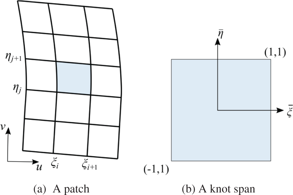
Figure 1: Mapping in the isogeometric space

By employing the NURBS basis functions, the acoustic potential and velocity are expressed as follows:

p(x)=∑i=1l∑j=1mRi,j,p,q(u(x),v(x))p~i,j,p,q(u(x),v(x))(19)

v(x)=∑i=1l∑j=1mRi,j,p,q(u(x),v(x))v~i,j,p,q(u(x),v(x))(20)

where l and m are the number of control points, and p and q are the curve degrees in u and v directions, respectively. p~ and v~ are the coefficients of sound pressure and velocity associated with the control points, given that the control points may no longer lie on the boundary.

2.3 Discontinuous IGABEM

2.3.1 Corner Problem

In BEM, the existence and uniqueness of the normal vector n are required to solve the BIE. The boundary of the body structure is composed of multiple NURBS patches in the interior noise calculation of the automotive passenger compartment, where the normal vector may not be unique at the junction of different NURBS patches. Moreover, the boundary conditions are no longer one single type on the boundary, but consist of Neumann and Robin conditions at the same time. As a result, the parameter values of the boundary conditions cannot be determined at nodes shared by neighbor elements. Numerical experiments show that if the parameter values (normal vector n or values of the primary variables and their derivatives) on either side of neighbor elements are considered boundary values in the calculation, then a false value is obtained on the other side, leading to unacceptable error especially at the corner nodes [31]. This condition is the corner problem in BEM. In general, corner problems may take the following forms:

(1)   Geometric corner problem: the boundary of the geometry is unsmooth and the normal vector has multiple directions at the nodes shared by neighbor elements, such as a geometric tip shown in Fig. 2.

(2)   Physical corner problem: the types or the parameter values of boundary conditions on neighbor elements are different, and the value of boundary conditions cannot be determined at the junction of neighbor elements. These nodes at the junctions are called physical corner nodes, as shown in Fig. 3. If continuous elements are still used to express the variables and derivatives in such situations, then large calculation error becomes inevitable, especially at the corner nodes.

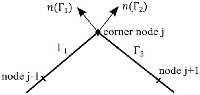
Figure 2: Geometric corner problem

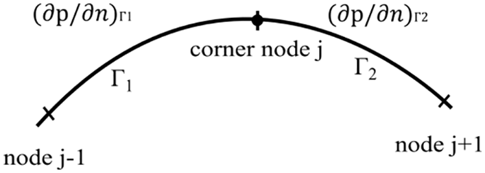
Figure 3: Physical corner problem

Many methods addressing corner problems have been proposed in BEM [32–34], among which the “double nodes” method is efficient and easy to implement. The “double nodes” method can be traced back to early BEM studies, such as Brebbia’s work [35] and subsequent studies [36]. The idea of “double nodes” is to place two nodes at positions close to the corner node on both sides of neighbor elements, as shown in Fig. 4. BIEs are established at the two nodes to avoid the inconsistence of normal vectors or boundary conditions at the corner nodes. Different from FEM, BEM does not require the continuity of physical quantities over the neighbor elements, thereby enabling the application of “double nodes” in BEM [20].

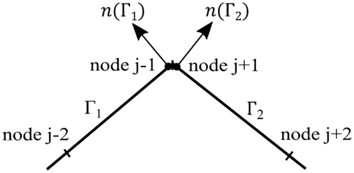
Figure 4: Double nodes

2.3.2 Discontinuous IGABEM Formulation

To date, there are only a few studies on corner problems in the development of IGABEM. In 3D elastic problems, Scott et al. [37] and Marussig et al. [38] used discontinuous elements to express the primary variable of traction. Nevertheless, the expression of displacement remained continuous. Andrade et al. [39] proposed an enriched IGABEM for 2D fatigue crack growth problem by inserting repetitive knots to increase the discontinuity of the NURBS, in which the basic functions of NURBS are changed as well. Wang et al. [40] established a nonsingular IGABEM based on multi-patches for elastic problems. Wang [41] improved the continuous IGABEM based on the idea that the geometric parameter space and physical space are independent of each other. Nevertheless, both studies are based on piecewise interpolation, where different spline interpolations are used to discretize the geometric and physical fields, thereby increasing the computational complexity in solving the corner problem.

Invoking the idea of “double nodes” method in BEM, the authors’ previous work [21] has presented a discontinuous IGABEM formulation by introducing discontinuous elements into the continuous IGABEM. In discontinuous elements as shown in Fig. 5, the nodes are located inside the elements, increasing the flexibility in mesh grading. In a discontinuous model, multiple control points can exist at the same location, each belonging to a different patch. Hence, the normal vector or variable at the points on the patch perimeter can be determined uniquely, and the geometric and physical corner problems are avoided fundamentally. Building such discontinuous element without changing the NURBS basis function is simple and straightforward. Three collocation strategies are compared in our earlier work, where the uniform collocation scheme has been proven to outperform the Legendre polynomials and modified-Greville abscissae strategies in terms of accuracy and converge speed.

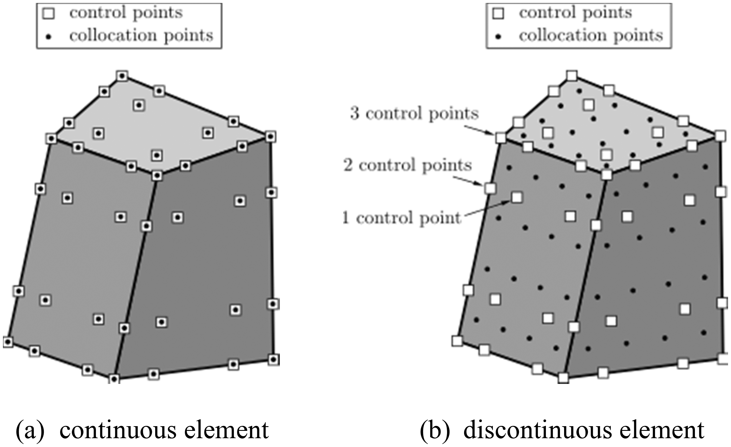
Figure 5: Isogeometric boundary elements

In discontinuous IGABEM, the jump term C(s) in Eq. (12) at all points yields C(s)=0.5, because all the collocation points are located inside the element. Liu’s [42] identities are used as follows:

∫Γ∂G¯(s,x)∂nd Γ(x)=−0.5(21)

with

G¯(s,x)=14πr(22)

The fundamental solutions of boundary element formulations in Eq. (12) can be reconstructed into the following regularized form:

−∫Γ∂G¯(s,x)∂np(s)d Γ(x)=∫Γ[iωρG(s,x)v(x)−p(x)∂G(s,x)∂n]d Γ(x)(23)

The singularity of the kernel in Eq. (23) is reduced from strong to weak; it can be effectively canceled by the Telles transformation [43]. Employing the NURBS basis function, Eq. (23) is discretized in an expansion form as follows:

∑e=1E∑i=1l∑j=1mPeij(x)peij−∑e=1E∑i=1l∑j=1mP¯eij(s)peij=∑e=1E∑i=1l∑j=1mQeij(x)iωρveij(24)

with

Peij=∫−11∫11∂G(ξ¯,η¯)∂nReij(ξ¯,η¯)Jeij(ξ¯,η¯)dξ¯dη¯(25)

P¯eij=∫−11∫11∂G¯(ξ¯,η¯)∂nRe^ij(ξ¯,η¯)Jeij(ξ¯,η¯)dξ¯dη¯(26)

Qeij=∫−11∫11G(ξ¯,η¯)Reij(ξ¯,η¯)Jeij(ξ¯,η¯)dξ¯dη¯(27)

where ξ¯=ξ¯(u,v), η¯=η¯(u,v), e^ is the element that source point s belongs to. Reij are the corresponding NURBS basis functions, and Jeij is the Jacobian from the mapping in Eq. (18). The two indices i, j refer to the bidirectional net of control points and associated basis functions in an element.

Taking the point s to lie at each node in turn, the collocation form of the BIE can be expressed as a matrix form:

Hu=Gq(28)

where nodal values of p(x) and v(x) are contained in vectors u and q, respectively, and the component of matrix H and G can be evaluated as follows:

H=∑e=1E∑i=1l∑j=1m∫−11∫−11∂G(ξ¯(x),η¯(x))∂nReijJeijdξ¯dη¯−δee^∑e=1E∑i=1l∑j=1m∫−11∫−11∂G¯(ξ¯(s),η¯(s))∂nRe^ijJeijdξ¯dη¯(29)

G=iρω∑e=1E∑i=1l∑j=1m∫−11∫−11G(ξ¯(x),η¯(x))ReijJeijdξ¯dη¯(30)

where δee^ is the Kronecker’s delta function, as follows:

δee^={ 10 e=e^e≠e^(31)

By moving all the unknowns and related coefficients to the left-hand side of the equation and all the known and related coefficients to the right-hand side, a linear equation system is obtained as follows:

Aμ=b(32)

where A is an unsymmetrical and fully populated matrix; vector μ contains all unknown values, whereas vector b is constructed by all known coefficients and corresponding associated terms. Eq. (32) is a linear system, which can be solved directly or iteratively. Marburg et al. [44] studied the performance of iterative solvers for acoustic problems, and the generalized minimal residual (GMRES) turned out to be the most effective and stable in the calculation of interior noise problem. Hence, this study follows Marburg’s work to employ GMRES as the iterative solver in the following calculation.

The discontinuous IGABEM lends itself to parallel implementations because every term in the coefficient matrices H and G has only one single contribution from a single integral over an element. Thus, the combination of the parallel technique enables the discontinuous IGABEM to be more efficient than conventional continuous scheme. The discontinuous IGABEM has shown to be more accurate and converges faster than the continuous BEM and IGABEM in an actual car passenger compartment subjected to Robin and Neumann boundary conditions in the authors’ previous work. In the present work, we combine the discontinuous IGABEM and the PACA to build an easily implementable and efficient tool to identify the critical panels that contribute most to the sound pressure at an observing point.

3  Panel Acoustic Contribution Analysis

The current PACA mainly consists of the experiment-based and numerical methods, both of which are timing and effort consuming in dealing with the large scale and complicated engineering problems. In this work we combine the discontinuous IGABEM with PACA, aiming to build a scheme that can precisely and efficiently evaluate the acoustic contribution of each panel for automotive acoustic problems.

3.1 Interior Sound Pressure Evaluation

According to the explanation in Section 2.2, the jump-term at the interior point t yields C(t)=1. Substituting C(t)=1 into Eq. (12) and taking the sound pressure p and velocity v at the boundary as the known boundary conditions, the sound pressure at the interior point t can be calculated by the following:

p(t)=hp+gv(33)

The component of coefficient vectors h and g can be evaluated by the following:

h=−∑e=1E∑i=1l∑j=1m∫−11∫−11∂G(ξ¯(x),η¯(x))∂nReijJeijdξ¯dη¯(34)

g=iρω∑e=1E∑i=1l∑j=1m∫−11∫−11G(ξ¯(x),η¯(x))ReijJeijdξ¯dη¯(35)

Thus, the interior sound pressure at any field point can be evaluated by Eq. (33) when the sound pressure and velocity of the structure surface are obtained. In engineering practice, measuring the sound pressure on a logarithmic scale is more desirable, among which the sound pressure level (SPL) is the most commonly used. The SPL with units of decibels is evaluated from sound pressure as follows:

SPL=10log10⁡|p2||p2ref|=20log10⁡|p||pref|(36)

The threshold of human hearing pref=2.0×10−5Pa is considered the reference sound pressure.

3.2 Panel Acoustic Contribution Analysis Based on the Discontinuous IGABEM

The acoustic contribution of a panel refers to the contribution accounting for the interaction between the panel vibrations and the sound pressure at a certain interior point. The automotive passenger compartment consists of different panels, whose contribution is influenced by the structure size, position and orientation. In this section, an acoustic contribution ratio is defined to visually describe the contribution analysis of a vibrating panel to the sound pressure at the point of interest.

In IGABEM, a patch is a subdomain in which the element types and material properties are uniform. NURBS patches are considered panels to divide the structure boundary and analyze the relative acoustic contribution. The sound pressure p(t) at an interior point t can be expressed as a summation of the sound pressure caused by all panels [10,45], as follows:

p(t)=∑e=1Epe(t)(37)

where E is the total number of the panels, pe(t) denotes the sound pressure generated by the e-th panel at the observing point, which can be expressed as a summation of sound pressure contributed by all the nodes on the investigated panel as follows:

pe(t)=∑i=1l∑j=1mpij(38)

where n and m are the number of the basis functions in two parametric directions on the patch, and pij denotes the associated sound pressure at the node; it can be obtained through Eq. (19). A panel acoustic contribution ratio ce(t) is defined as the projection of the sound pressure generated by the patch to the total internal pressure as follows:

ce(t)=|pe(t)||p(t)|cos⁡θ(39)

where θ is the phase difference of pe(t) and p(t). According to Euler’s formula, cos⁡θ=Re(eiθ) can be obtained, thus, the contribution ratio ce(t) can be calculated as follows:

ce(t)=Re(|pe(t)||p(t)||p(t)|2eiθ)=Re(|pe(t)|⋅p∗(t)|p(t)|2)(40)

where “Re” denotes the real component of a complex number, and the superscript “∗” indicates the complex conjugate. p(t) and pe(t) can be calculated by Eqs. (33) and (38), respectively.

The diagram of the definition of panel contribution is illustrated in Fig. 6. The contribution ratio ce(t) can either be positive or negative, representing increasing and cancelation effects of energy at the observing point. The sound pressure at t increases if the vibrating velocity of the positive contribution panels increases. By contrast, the sound pressure at t decreases if the vibrating velocity of the negative contribution panels increases. If the contribution ratio of the panel is close to zero, then it has no significant contribution to the sound pressure at t. The coefficient vectors p(t) and pe(t) in calculating ce(t) have already generated in the calculation of the interior sound pressure at t. Therefore, estimating the individual’s contribution is easier and straightforward, compared with the traditional experiment-based schemes.

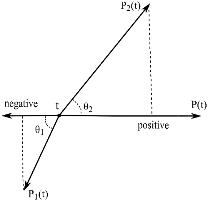
Figure 6: Diagram of definition of panel contribution

Therefore, the implementation of PACA using discontinuous IGABEM consists of two steps. The first step is to obtain the sound pressure p(t) over the boundary and pe(t) at the observing point by solving Eqs. (32) and (33), respectively. The second step is to evaluate the contribution ratio ce(t) in Eq. (40) of each panel directly by reusing the coefficient matrix generated in the first step.

Taking advantage of discontinuous IGABEM, the proposed PACA method can be accelerated by the parallel technique. In the following section, the PACA with the proposed method is conducted based on two numerical examples.

4  Numerical Examples

Two numerical examples are illustrated in this section to validate the accuracy and efficiency of the PACA with discontinuous IGABEM. The uniform collocation method is used to determine the location of the collocation points, following our earlier work [21]. Quadratic shape functions are applied in BEM analysis, and the quadratic uniform knot vectors are used in the NURBS representation. All the calculations are conducted based on MATLAB platform, where the “parfor” parallel technique is used instead of regular “for” to lead the loops in the calculation of H and G matrix in discontinuous IGABEM. “Parfor” is a tool offered by MATLAB to implement the parallel calculation in a multicore computer. Being different from the “for” keyword, loops lead by “parfor” can run in parallel on multiple processors, which accelerate the calculation remarkably. The schematic of “parfor” is illustrated in Fig. 7.

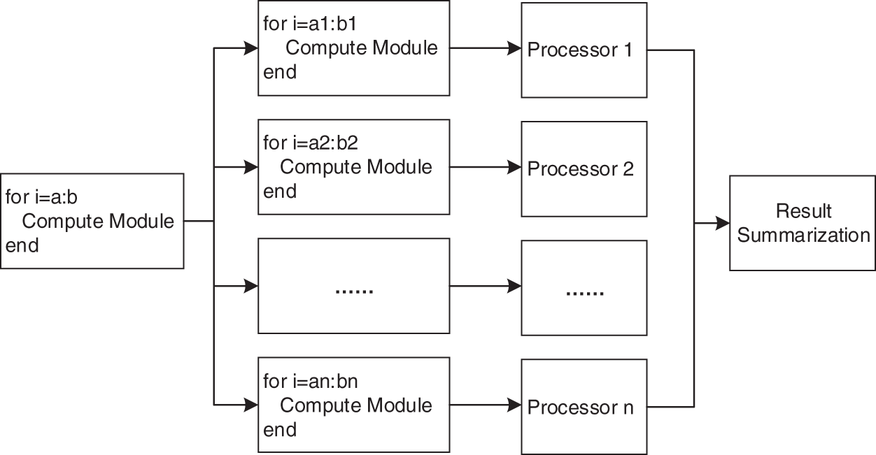
Figure 7: Schematic of “parfor”

GMRES is considered the solver in the calculation of the final matrix equation in BEM and discontinuous IGABEM. The air density ρ is 1.29 kg/m3, the sound speed c is 340 m/s, and the residual error of GMRES is 10−3. The results based on the proposed method and the conventional BEM with Lagrange discretization are compared.

4.1 Simple Cavity Model

The first simple cavity model consists of 10 flat panels as shown in Fig. 8. The geometric parameter of the structure is shown in Table 1. All the panels are numbered in a manner shown in Fig. 9. Point A is the intersection point of panel No. 1, No. 2 and No. 7. The bottom panel No. 6 is located on the xy plane, and the projection of point A on the xy plane is the origin of coordinates. The BE model using the Lagrange polynomial elements and NURBS model are illustrated in Fig. 10, containing 2906 and 3000 degrees of freedom (DOF), respectively. The point located at the (0.7, 0.8, 1.4 m) is selected as the observing point, where the sound pressure is evaluated using conventional BEM and discontinuous IGABEM.

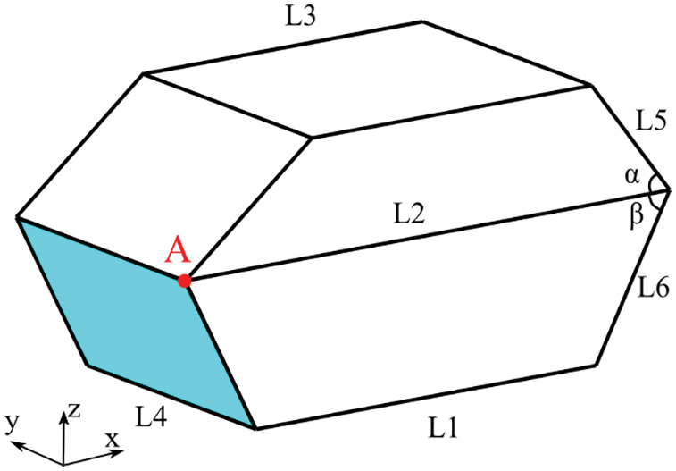
Figure 8: Structure of the simple cavity

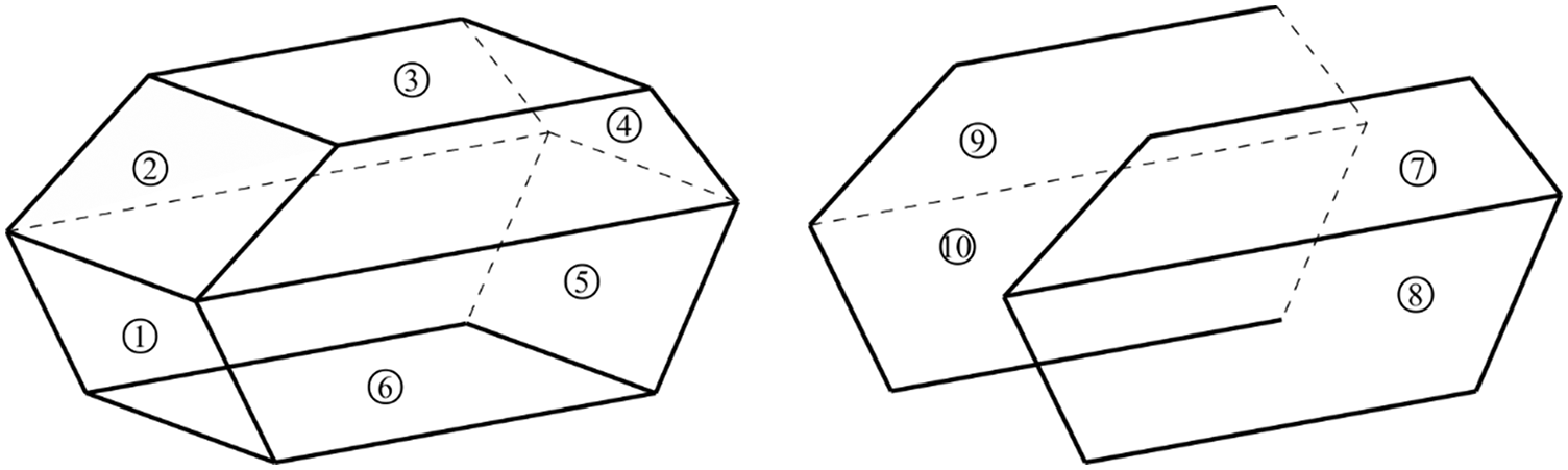
Figure 9: Number of the panels of the simple cavity

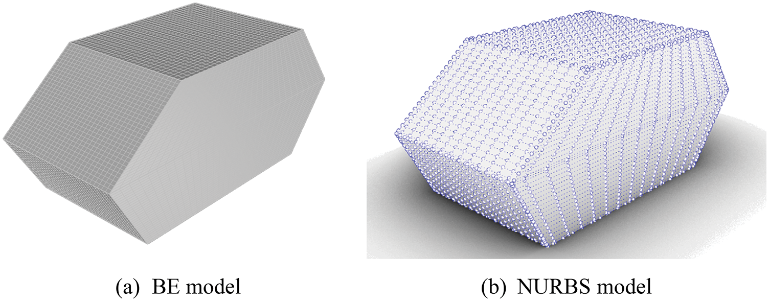
Figure 10: Discretized simple cavity

4.1.1 Interior Sound Pressure Evaluation

A uniform unit velocity with vs=1mm/s is applied on panel No. 1, whereas the remaining panels subjected to a uniform impedance boundary condition are obtained as follows:

Y=1ρcff0(41)

where f0=2800Hz, which is an average experimental parameter from Marburg et al.’s [46] work. The acoustic admittance Y and impedance Z yield the reciprocal relationship as Z=1/Y.

With a step size of 2 Hz, the sound pressure on the surface and at the observing point within the frequency range from 50 to 250 Hz are evaluated, using Eqs. (24) and (33), respectively. The comparison of the interior sound pressure at the observing point using conventional BEM and discontinuous IGABEM is shown in Fig. 11. The finding indicates that the accuracy of discontinuous IGABEM coincides highly with the conventional BEM in terms of critical frequency and corresponding SPL within the calculated frequency range.

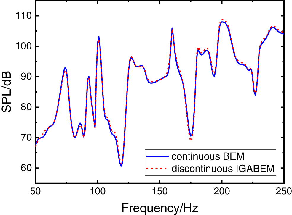
Figure 11: Comparison of SPL at the observing point of the simple cavity

4.1.2 Panel Acoustic Contribution Analysis

The acoustic contribution of the panels can be identified when the interior noise is obtained. At the frequency of 100 Hz, which is one of the peak frequencies, the acoustic contribution of each panel is evaluated using Eq. (40), and the result is shown in the Fig. 12. High coincidence of the acoustic contribution is observed for every single panel by using BEM and discontinuous IGABEM. At the frequency of 100 Hz, panel No. 1 contributes most to the sound pressure at the observing point. The radiation acoustic field inside the cavity is generated by the vibration of panel No. 1, and the sound pressure at the observing point can be reduced by eliminating the vibration of the critical panel. The largest relative error of the two methods is 7.31%, whereas the smallest relative error is 0.01%.

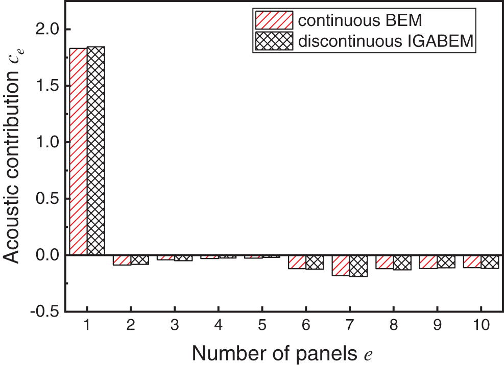
Figure 12: PACA of the simple cavity at 100 Hz

The computing time of both methods are compared: the entire time of the PACA based on BEM is 731.96 s, whereas the discontinuous IGABEM is 95.23 s. The DOF of the two models are nearly the same, but the computing time of the discontinuous IGABEM is two orders of magnitudes less than the conventional BEM.

4.2 Automotive Compartment Model

An automotive passenger compartment is studied as a second example to illustrate the accuracy and efficiency of the proposed method, as shown in Fig. 13. The blue panel represents the dash board, the red panels represent the door, floor, and roof of the automotive body attached with lining material, and the gray panels represent the window glass. The discretized model based on the Lagrange elements consists of 11250 DOF (Fig. 14a), whereas the NURBS model consists of 11380 DOF (Fig. 14b).

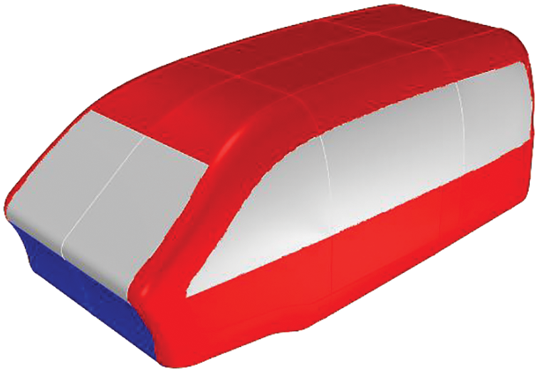
Figure 13: Structure of the automotive passenger compartment

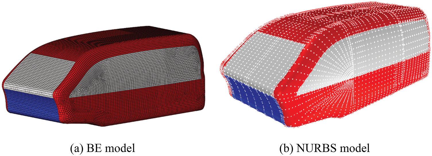
Figure 14: Discretized passenger compartment

The automotive body is divided into 24 panels, including the roof, dashboard, side doors and the floorboard. The numbers of the panels are shown in Fig. 15.

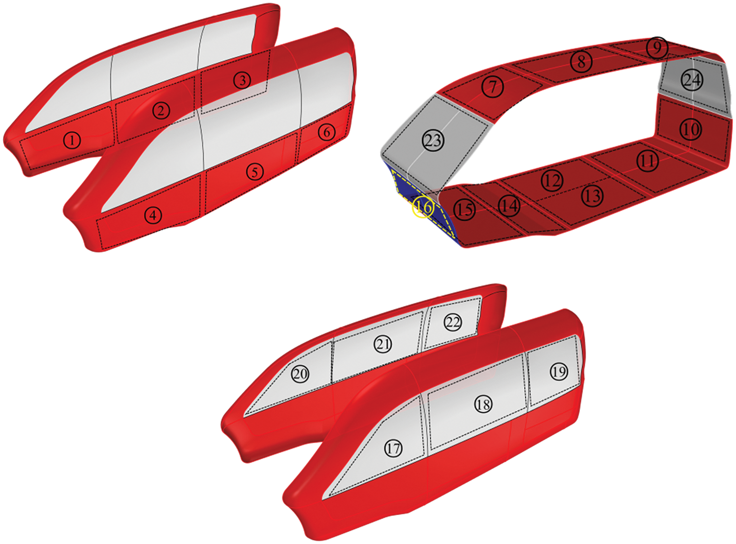
Figure 15: Number of the panels of the automotive body

4.2.1 Interior Sound Pressure Evaluation

The interior sound field in the automotive acoustic cavity can be simulated subject to three types of boundary conditions, as follows:

(1)   If a structure surface is oscillating, e.g., the vehicle dashboard, then the boundary condition can be expressed as a Neumann condition, as follows:

p=−iρωv(42)

where ω=2πc/λ is the circular frequency, and v is the amplitude of the normal component of the velocity on the surface. In this study, we take wave length λ=5 and v=1.452m/s following an experimental result [47].

(2)   If a structure surface is fully reflective, e.g., the window glass, then the boundary condition can be expressed as a uniform Neumann condition, as follows:

p=0(43)

(3)   For absorbing boundaries, e.g., the interior lining material of the passenger compartment, the boundary condition can be expressed as a Robin condition, as follows:

p=Zv(44)

In this work, the first Neumann boundary condition is applied on the blue panels, representing the dashboard. The second Neumann boundary condition is applied on the gray panels, representing the window glass. The third Robin condition is applied on the remaining panels, representing the inner lining material of the compartment, where acoustic impedance Z or admittance Y is obtained, following Eq. (41).

The sound pressure at the observing point is calculated using the conventional BEM and the discontinuous IGABEM in frequency band from 40 to 200 Hz, with the step size of 2 Hz. The comparison between two methods is shown in Fig. 16, from which the highly coincident results of the BEM and the discontinuous IGABEM are observed as well. Slight difference in the SPL at the peak frequencies is observed, probably caused by the error of the geometry discretization in the traditional BEM. On the contrary, the discontinuous IGABEM has no geometry error, because the analysis is based on the exact geometry representation.

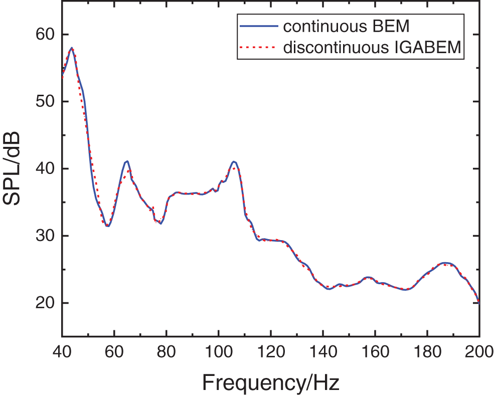
Figure 16: Comparison of SPL at the observing point of the automotive compartment

4.2.2 Panel Acoustic Contribution Analysis

The acoustic contribution of the panels at one of the peak frequencies of 106 Hz is investigated in the following section. Fig. 17 illustrates the comparison of the PACA result based on the conventional BEM and discontinuous IGABEM. It indicates that the contribution ratio of every panel based on the two methods is very close. The largest relative error of the two methods is 6.94%, whereas the smallest relative error is 0.01%. Panel No. 16 representing the dashboard contributes the most to the sound pressure at the observing point, and this result can guide the structure acoustic optimization to improve the automotive NVH performance.

Figure 17: PACA of the automotive compartment at 106 Hz

The computing time of both methods at the frequency of 106 Hz is compared. The total time using conventional BEM is 7065.54 s, whereas the time of discontinuous IGABEM is 885.71 s. The PACA based on the discontinuous IGABEM is evidently faster than the conventional BEM, even without considering the time of the mesh generation and refinement that it saves compared with BEM. Hence, the two numerical examples indicate that the proposed method is not only easier to implement but also more efficient than the conventional PACA schemes, showing great potential of its application in automotive acoustics.

5  Experimental Validation

A sound response experiment on the interior acoustic field of a Q235 steel box is designed to validate the accuracy of the interior noise evaluation based on discontinuous IGABEM. The size of the steel box is 890 mm × 690 mm × 460 mm, as shown in Fig. 18. The bottom panel is as thick as 30 mm, and the four side panels are as thick as 20 mm. All these panels are sufficiently thick to be regarded as rigid walls. The top panel is as thin as 2 mm, which is fixed on the side panels though four steel bars with cross section of 20 mm × 20 mm, using sealing gaskets and bolts. The experiment is conducted in a semi-anechoic chamber, with cut-off frequency of 50 Hz and background noise of 20 dB, as shown in Fig. 19.

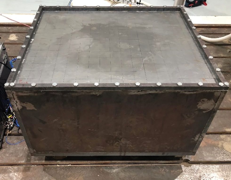
Figure 18: Structure of the Q235 steel box

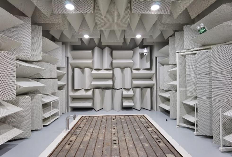
Figure 19: Semi-anechoic chamber

A volume sound source shown in Fig. 20a is placed in the center of the bottom panel inside the box, which can produce the white noise signal with a bandwidth of 0–250 Hz. Excited by the sound signal, the top panel vibrates and generates a radiated acoustic field inside the box. The directions of the width, length, and height of the box are set as x, y, and z axis, respectively, and the test points are evenly placed on the top panel along the x and y directions with an interval of 50 mm, generating 192 test points in total. The acceleration sensors are placed at the test point to measure the normal velocity of each point.

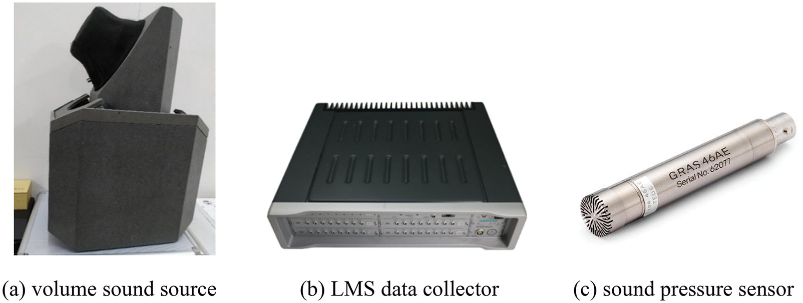
Figure 20: Experiment devices

LMS Test.Lab is used to process the experimental signal, and the corresponding device is LMS SCM05 40-channel data collector, as shown in Fig. 20b. The acceleration sensor PCB356A25 is used to measure the normal velocity of each test point. The sound pressure is measured using GRAS 46AE sound pressure sensor, shown in Fig. 20c, with a measurement range of 3.15 Hz–20 kHz. HS6020 sound calibrator is used to calibrate the sensitivity of sound pressure sensor prior to conducting the experiment.

Power amplifier, signal collector, personal computer, and other devices are connected following the test system diagram shown in Fig. 21. The experiment is setup, as shown in Fig. 22. Taking the internal point (400, 300, 100 mm) as the observing point, the sound pressure sensor is placed at the corresponding location.

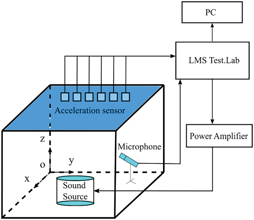
Figure 21: Experiment system

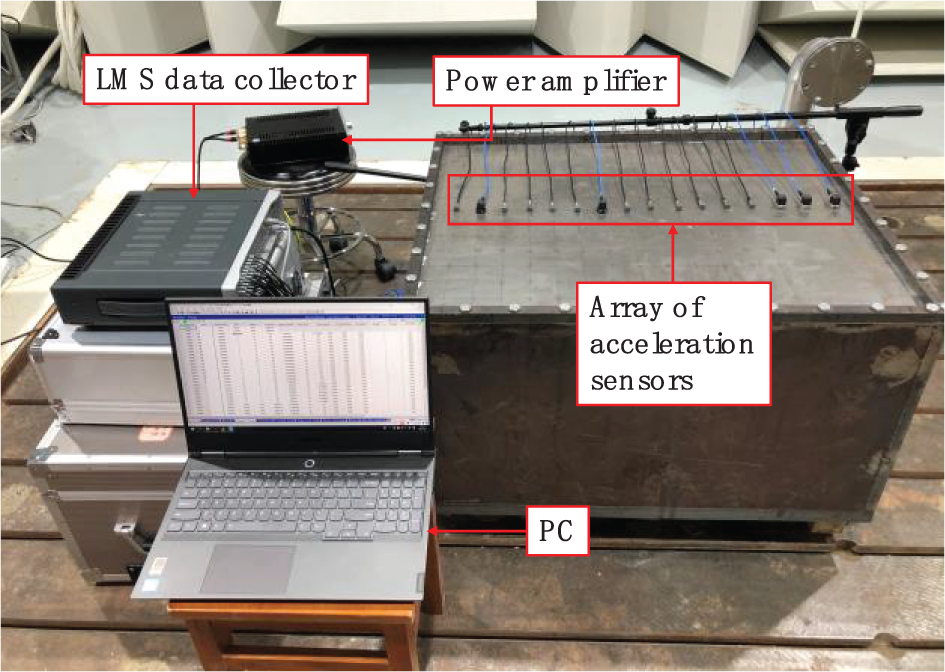
Figure 22: Velocity measurement of the top panel

The experimental values of the velocity at each test node on the top panel are considered the boundary conditions to calculate the sound pressure of the boundary. Then, the sound pressure at the observing point is evaluated using discontinuous IGABEM with a step size of 2 Hz. The comparison of experimental and calculated results is shown in Fig. 23. This finding indicates that the trend of the measured sound pressure at the observing point is consistent with the calculated value within the frequency range of 0–250 Hz. The amplitudes of the SPL are close, exhibiting slight difference at the peak frequencies, which could be caused by the measurement error in particle velocity brought on by the weight of the acceleration sensors. The maximum error between the measured and the calculated results at the peak is 3.42 dB, and the minimum error is only 0.074 dB, thereby demonstrating that the proposed discontinuous IGABEM is reliable and accurate in predicting the interior noise of the radiated acoustic field.

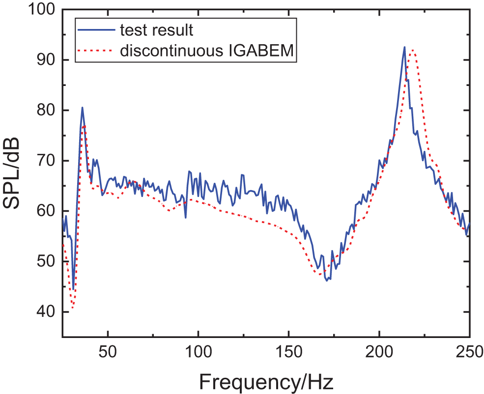
Figure 23: Comparison of the experimental and calculated result of the sound pressure

6  Conclusions

A PACA scheme using discontinuous IGABEM is presented in this work. Discontinuous IGABEM has shown the ability to more efficiently approximate engineering acoustic problems where geometry and primary variables exhibit large gradients or discontinuities. The acoustic contribution of each panel is investigated by the proposed method in two steps. First, the interior sound pressure is evaluated by discontinuous IGABEM through a regularization from BIE with weak singularity. Second, the contribution of the individual panel to the sound pressure at any field point is identified through a defined contribution ratio. When the sound pressure at the observing point is obtained, the contribution ratio can be estimated directly by reusing the coefficient matrix that has been generated in the first step. The utilization of the parallel technique enables the proposed method to be highly efficient. Numerical examples confirm that the calculation time of PACA based on the discontinuous IGABEM method is one order of magnitude less than the conventional method with close DOF. The proposed method shows great potential for the discontinuous IGABEM in the identification of critical panels, thereby improving the efficiency of the structure acoustic optimization in automotive engineering.

Funding Statement: This work is funded by the National Natural Science Foundation of China (Grant No. 52175111), which is received by Liu, Z. The URL to the sponsors’ website is https://www.nsfc.gov.cn/.

Conflicts of Interest: The authors declare that they have no conflicts of interest to report regarding the present study.

References

1. Marburg, S., Hardtke, H. (2003). Investigation and optimization of a spare wheel well to reduce vehicle interior noise. Journal of Computational Acoustics, 11(3), 425–449. DOI 10.1142/S0218396X03002036. [Google Scholar] [CrossRef]
2. Cheng, G., Herrin, D. W., Stencel, J. (2022). Acoustic radiation prediction using panel contribution analysis combined with scale modeling. Applied Acoustics, 186, 108458. DOI 10.1016/j.apacoust.2021.108458. [Google Scholar] [CrossRef]
3. Automated Analysis Corporation (1994). COMET/ACOUSTICS user’s manual, version 2.1. Automated Analysis Corporation, Ann Arbor, Michigan. [Google Scholar]
4. Computational Mechanics BEASY (1994). BEASY User Guide, Computational Mechanics BEASY, Southampton, England. [Google Scholar]
5. Ishiyama, S. I., Imai, M., Maruyama, S. I., Ido, H., Sugiura, N. et al. (1988). The applications of ACOUST/BOOM-a noise level predicting and reducing computer code. SAE Transactions, 97, 976–986. DOI 10.2307/44724784. [Google Scholar] [CrossRef]
6. Plunt, J. (1998). Strategy for transfer path analysis (TPA) applied to vibro-acoustic systems at medium and high frequencies. Proceedings of the 23rd International Conference on Noise and Vibration Engineering, pp. 16–18. Leuven, Belgium. [Google Scholar]
7. Hald, J., Tsuchiya, M., Blaabjerg, C., Ando, H., Yamashita, T. et al. (2006). Panel contribution analysis using a volume velocity source and a double layer array with the SONAH algorithm. INTER-NOISE and NOISE-CON Congress and Conference Proceedings, pp. 1465–1474. Honolulu, USA. [Google Scholar]
8. Wolff, O. (2007). Fast panel noise contribution analysis using large PU sensor arrays. 36th International Congress and Exhibition on Noise Control Engineering, pp. 28–31. Istanbul, Turkey. [Google Scholar]
9. Wang, Y., Qin, X., Li, L., Liu, H., Huang, J. (2016). The noise control of minicar body in white based on acoustic panel participation method. Journal of Vibroengineering, 18(2), 1332–1345. [Google Scholar]
10. Zhang, Y. K., Lee, M., Stanecki, P. J., Brown, G. M., Allen, T. E. et al. (1995). Vehicle noise and weight reduction using panel acoustic contribution analysis. SAE Transactions, 104, 2411–2421. DOI 10.2307/44729306. [Google Scholar] [CrossRef]
11. Hughes, T. J. R., Cottrell, J. A., Bazilevs, Y. (2005). Isogeometric analysis: CAD, finite elements, NURBS, exact geometry and mesh refinement. Computer Methods in Applied Mechanics and Engineering, 194(39−41), 4135–4195. DOI 10.1016/j.cma.2004.10.008. [Google Scholar] [CrossRef]
12. Lian, H., Chen, L., Lin, X., Zhao, W., Bordas, S. P. A. et al. (2022). Noise pollution reduction through a novel optimization procedure in passive control methods. Computer Modeling in Engineering & Sciences, 131(1), 1–18. DOI 10.32604/cmes.2022.019705. [Google Scholar] [CrossRef]
13. Simpson, R. N., Scott, M. A., Taus, M., Thomas, D. C., Lian, H. (2014). Acoustic isogeometric boundary element analysis. Computer Methods in Applied Mechanics and Engineering, 269, 265–290. DOI 10.1016/j.cma.2013.10.026. [Google Scholar] [CrossRef]
14. Peng, X., Lian, H., Ma, Z., Zheng, C. (2022). Intrinsic extended isogeometric analysis with emphasis on capturing high gradients or singularities. Engineering Analysis with Boundary Elements, 134, 231–240. DOI 10.1016/j.enganabound.2021.09.022. [Google Scholar] [CrossRef]
15. Vazquez, R., Buffa, A., di Rienzo, L., Li, D. (2014). Isogeometric finite elements with surface impedance boundary conditions. IEEE Transactions on Magnetics, 50(2), 429–432. DOI 10.1109/TMAG.2013.2280293. [Google Scholar] [CrossRef]
16. Wang, D., Zhang, H., Xuan, J. (2012). A strain smoothing formulation for NURBS-based isogeometric finite element analysis. Science China Physics, Mechanics and Astronomy, 55(1), 132–140. DOI 10.1007/s11433-011-4528-1. [Google Scholar] [CrossRef]
17. Wang, J., Jiang, F., Zhao, W., Chen, H. (2021). A combined shape and topology optimization based on isogeometric boundary element method for 3D acoustics. Computer Modeling in Engineering & Sciences, 127(2), 645–681. DOI 10.32604/cmes.2021.015894. [Google Scholar] [CrossRef]
18. Gilvey, B., Trevelyan, J., Hattori, G. (2020). Singular enrichment functions for helmholtz scattering at corner locations using the boundary element method. International Journal for Numerical Methods in Engineering, 121(3), 519–533. DOI 10.1002/nme.6232. [Google Scholar] [CrossRef]
19. Ji, D., Lei, W., Li, H. (2016). Corner treatment by assigning dual tractions to every node for elastodynamics in TD-BEM. Applied Mathematics and Computation, 284(C), 125–135. DOI 10.1016/j.amc.2016.02.059. [Google Scholar] [CrossRef]
20. Zhang, X. S., Zhang, X. X. (2002). Coupling FEM and discontinuous BEM for elastostatics and fluid-structure interaction. Engineering Analysis with Boundary Elements, 26(8), 719–725. DOI 10.1016/S0955-7997(02)00031-0. [Google Scholar] [CrossRef]
21. Sun, Y., Trevelyan, J., Hattori, G., Lu, C. (2019). Discontinuous isogeometric boundary element (IGABEM) formulations in 3D automotive acoustics. Engineering Analysis with Boundary Elements, 105, 303–311. DOI 10.1016/j.enganabound.2019.04.011. [Google Scholar] [CrossRef]
22. Piegl, L. A., Tiller, W. (1995). The NURBS book. New York, USA: Springer. [Google Scholar]
23. Rogers, D. F. (2001). An introduction to NURBS: With historical perspective. San Francisco: Morgan Kaufmann Publishers. [Google Scholar]
24. Boor, C. D. (1972). On calculating with B-splines. Journal of Approximation Theory, 6(1), 50–62. DOI 10.1016/0021-9045(72)90080-9. [Google Scholar] [CrossRef]
25. Cox, M. G. (1972). The numerical evaluation of B-splines. IMA Journal of Applied Mathematics, 10(2), 134–149. DOI 10.1093/imamat/10.2.134. [Google Scholar] [CrossRef]
26. Peng, X., Lian, H. (2022). Numerical aspects of isogeometric boundary element methods: (nearly) singular quadrature, trimmed NURBS and surface crack modeling. Computer Modeling in Engineering & Sciences, 130(1), 513–542. DOI 10.32604/cmes.2022.017410. [Google Scholar] [CrossRef]
27. L, Y. L., Stroud, A. H., Secrest, D. (1966). Gaussian quadrature formulas. Mathematics of Computation, 21(97), 125–126. DOI 10.2307/2003493. [Google Scholar] [CrossRef]
28. Guiggiani, M., Krishnasamy, G., Rudolphi, T. J., Rizzo, F. J. (1992). A general algorithm for the numerical solution of hypersingular boundary integral equations. Journal of Applied Mechanics, 59(3), 604–614. DOI 10.1115/1.2893766. [Google Scholar] [CrossRef]
29. Silva, J. J. (1994). Acoustic and elastic wave scattering using boundary elements. Southampton, UK and Boston, USA: Computational Mechanics Publications. [Google Scholar]
30. Rong, J., Wen, L., Xiao, J. (2014). Efficiency improvement of the polar coordinate transformation for evaluating BEM singular integrals on curved elements. Engineering Analysis with Boundary Elements, 38, 83–93. DOI 10.1016/j.enganabound.2013.10.014. [Google Scholar] [CrossRef]
31. Yao, S. (1995). Boundary element method and its applications in engineering. Beijing, China: National Defense Industry Press. [Google Scholar]
32. Paula, F. A. D., Telles, J. C. F. (1989). A comparison between point collocation and galerkin for stiffness matrices obtained by boundary elements. Engineering Analysis with Boundary Elements, 6(3), 123–128. DOI 10.1016/0955-7997(89)90025-8. [Google Scholar] [CrossRef]
33. Bialecki, R., Dallner, R., Kuhn, G. (1993). New application of hypersingular equations in the boundary element method. Computer Methods in Applied Mechanics and Engineering, 103(3), 399–416. DOI 10.1016/0045-7825(93)90130-P. [Google Scholar] [CrossRef]
34. Chaudonneret, M. (1978). On discontinuity of stress vector in the boundary integral equation method for elastic analysis. In: Recent advances in boundary element methods, pp. 194–195. Plymouth, London, UK: Pentech Press. [Google Scholar]
35. Brebbia, C. A., Dominguez, J. (1977). Boundary element methods for potential problems. Applied Mathematical Modelling, 1(7), 372–378. DOI 10.1016/0307-904X(77)90046-4. [Google Scholar] [CrossRef]
36. Parreira, P. (1988). On the accuracy of continuous and discontinuous boundary elements. Engineering Analysis with Boundary Elements, 5(4), 205–211. DOI 10.1016/0264-682X(88)90018-4. [Google Scholar] [CrossRef]
37. Scott, M. A., Simpson, R. N., Evans, J. A., Lipton, S., Bordas, S. P. A. et al. (2013). Isogeometric boundary element analysis using unstructured T-splines. Computer Methods in Applied Mechanics and Engineering, 254, 197–221. DOI 10.1016/j.cma.2012.11.001. [Google Scholar] [CrossRef]
38. Marussig, B., Zechner, J., Beer, G., Fries, T. (2015). Fast isogeometric boundary element method based on independent field approximation. Computer Methods in Applied Mechanics and Engineering, 284, 458–488. DOI 10.1016/j.cma.2014.09.035. [Google Scholar] [CrossRef]
39. Andrade, H. C., Trevelyan, J., Leonel, E. D. (2022). A NURBS-discontinuous and enriched isogeometric boundary element formulation for two-dimensional fatigue crack growth. Engineering Analysis with Boundary Elements, 134, 259–281. DOI 10.1016/j.enganabound.2021.09.019. [Google Scholar] [CrossRef]
40. Wang, Y. J., Benson, D. J. (2015). Multi-patch nonsingular isogeometric boundary element analysis in 3D. Computer Methods in Applied Mechanics & Engineering, 293, 71–91. DOI 10.1016/j.cma.2015.03.016. [Google Scholar] [CrossRef]
41. Wang, J. (2021). Research on the structural shape and topology optimization approaches for acoustic and vibro-acoustic problems based on the boundary element method (Ph.D. Thesis). University of Science and Technology of China, Hefei, China. [Google Scholar]
42. Liu, Y., Rudolphi, T. J. (1991). Some identities for fundamental solutions and their applications to weakly-singular boundary element formulations. Engineering Analysis with Boundary Elements, 8(6), 301–311. DOI 10.1016/0955-7997(91)90043-S. [Google Scholar] [CrossRef]
43. Telles, J. C. F. (1987). A self-adaptive co-ordinate transformation for efficient numerical evaluation of general boundary element integrals. International Journal for Numerical Methods in Engineering, 24(5), 959–973. DOI 10.1002/nme.1620240509. [Google Scholar] [CrossRef]
44. Marburg, S., Schneider, S. (2003). Performance of iterative solvers for acoustic problems. Part I. Solvers and effect of diagonal preconditioning. Engineering Analysis with Boundary Elements, 27(7), 727–750. DOI 10.1016/S0955-7997(03)00025-0. [Google Scholar] [CrossRef]
45. Xiao, Y., Chen, J., Hu, D., Jiang, F. (2015). Equivalent source method for identification of panel acoustic contribution in irregular enclosed sound field. Chinese Journal of Acoustics, 34(1), 49–66. [Google Scholar]
46. Marburg, S., Hardtke, H. J. (1999). Study on the acoustic boundary admittance. Determination, results and consequences. Engineering Analysis with Boundary Elements, 23(9), 737–744. DOI 10.1016/S0955-7997(99)00024-7. [Google Scholar] [CrossRef]
47. Zhu, J. (2005). On the simulation of the interior noise of a light-weight bus (Ph.D. Thesis). Jiangsu University, Zhenjiang, China. [Google Scholar]
Cite This Article
Copyright © 2023 The Author(s). Published by Tech Science Press.
This work is licensed under a Creative Commons Attribution 4.0 International License , which permits unrestricted use, distribution, and reproduction in any medium, provided the original work is properly cited.
Downloads
Citation Tools