
 Submit a Paper
 Propose a Special lssue
 Open Access
ARTICLE

On Nonlinear Conformable Fractional Order Dynamical System via Differential Transform Method
1 Department of Mathematics and Sciences, Prince Sultan University, Riyadh, 11586, Saudi Arabia
2 Department of Mathematics, University of Malakand, Chakdara Dir (L), Khyber Pakhtunkhwa, 18000, Pakistan
3 Department of Mathematics and Sciences, Prince Sultan University, Riyadh, 11586, Saudi Arabia
4 Department of Medical Research, China Medical University, Taichung, 40402, Taiwan
5 Department of Mathematics, Faculty of Arts and Sciences, Çankaya University, Ankara, 06790, Turkey
6 Department of Mathematical Sciences, UAE University, Al-Ain, 15551, United Arab Emirates
* Corresponding Author: Thabet Abdeljawad. Email:
Computer Modeling in Engineering & Sciences 2023, 136(2), 1457-1472. https://doi.org/10.32604/cmes.2023.021523
Received 18 January 2022; Accepted 26 September 2022; Issue published 06 February 2023
 View Full Text
 Download PDF
Abstract
This article studies a nonlinear fractional order Lotka-Volterra prey-predator type dynamical system. For the proposed study, we consider the model under the conformable fractional order derivative (CFOD). We investigate the mentioned dynamical system for the existence and uniqueness of at least one solution. Indeed, Schauder and Banach fixed point theorems are utilized to prove our claim. Further, an algorithm for the approximate analytical solution to the proposed problem has been established. In this regard, the conformable fractional differential transform (CFDT) technique is used to compute the required results in the form of a series. Using Matlab-16, we simulate the series solution to illustrate our results graphically. Finally, a comparison of our solution to that obtained for the Caputo fractional order derivative via the perturbation method is given.Keywords
The subject of fractional calculus is as old as classical calculus. However, the significant progress was made after 1970. This is due to the important applications in various branches of science and technology. In fact, during modelling of real world problems, those models which involve arbitrary order derivatives are found to be more suitable than classical order in many cases. Therefore, the area devoted to fractional order differential equations (FODEs) has been investigated very well (see for detail [1–7]). Furthermore, fractional calculus is a strong and efficient tool for modelling various nonlinear real-world phenomena. The mentioned calculus preserves heredity and non-locality properties, which are the important features. The aforesaid features have numerous applications in describing various processes and phenomena in the real world. Further, it is to be noted that the mentioned characteristics are different from those of traditional calculus developed by Newton and Lebnitz. For more informative applications, we refer to some published work such as [8–10]. Various new types of operators in fractional calculus have been introduced in the last two decades. It is worth mentioning that, results including uncertainty, nonlinearity, and other features, have been investigated increasingly in recent trials. In this regard, we refer to some new results such as in [11–13]. For more recent contributions and clarifications, we refer to some published work such as in [14–16]. For more some new updated applicable literature in different areas of engineering and sciences, one can refer to [17,18]).
Fractional derivatives have been defined in different ways in which the two definitions given by Reimann-Liouville and Caputo have gotten proper attention. Hence, the literature devoted to Reimann-Liouville and Caputo derivatives has been enriched by researchers very well. Unfortunately, the classical chain rule of calculus is not satisfied by these two derivatives. Therefore, some researchers in the last few years have introduced the concept of CFOD. The mentioned operator obeys a well-behaved chain rule an allows us to derive with respect to arbitrary order. Further, we state that the CFOD is free of memory terms and also called local derivatives of arbitrary order. In this regard, valuable work has been carried out by many researchers (we refer to [19–22]). In the literature, for some important work dealing with analytical results and qualitative theory of FODEs by using CFOD, we refer to [23–25]. More recently, some useful work has been published in the mentioned area by using CFOD (the details can be found in [26–32]).
It is worth mentioning that various analytical techniques like Laplace transform connected with the Adomian decomposition method, variational iteration procedure, differential transform method (DTM), perturbation, and homotopy analysis algorithms have been increasingly used to compute approximate solutions of various problems of FODEs and their systems (see [33–49]). In the first attempt, the Chinese mathematician, Zhou [50] introduced a semi-analytical technique called DTM in 1986. After that, DTM has been increasingly used to compute approximate solutions to ordinary as well as FODEs (see [51–54] and the references cited therein). On the other hand, existence theory is an important aspect which has been very well investigated in the last two decades for FODEs by using Reimann-Liouville and Caputo derivatives. But in the case of differential equations involving CFOD, the existence theory has very rarely been studied (very few articles are given such as [55,56]).
As usual, mathematical models are used as important tools to investigate and reflect various real-world processes in more detail. For instance, in the last two decades, researchers in the physical, social sciences, and engineering disciplines have given much attention to this rich and vital area. The famous Lotka and Volterra model was established in 1925, which was later on studied from different aspects. This dynamical model is considered to be a very interesting and famous in ecology, that shows the relationship between prey and predator. It has been studied in various articles for different purposes. In general, the model in [57] is recalled as
with
Here,
Currently, model (1) under the fixed coefficients
has been investigated by Das and his co-authors [57] by using the homotopy perturbation method (HPM) with Caputo derivative of fractional order
Inspired by model (3), we investigate the same system in the form
where
We establish some results about the existence and uniqueness of solutions for the considered problem by using some fixed point results. Existence theory is an important consequence of qualitative theory. Therefore, to investigate a dynamic problem, it must be ensured whether the problem exists and possesses a solution or not. The existence theory would tell us whether a dynamical problem has at least one solution, many solutions, or no solution at all. Therefore, numerous tools have been established to study existence theory, including fixed point theory and coincidence degree theories due to Mawhin and Schauder. Each has been extensively used in the literature to investigate various problems for the existence of solutions (see [59,60]). In order to study the approximate solutions to the system (4), we extend DTM as applied in [61] under CFOD. Some biological applications of mathematical models can be seen in [62–64]. We provide the evidence that the aforementioned techniques are rapidly convergent. Actually, it is efficient and easy to implement when compared to other analytical methods. Some frequent results in this regards are cited here as [65–67]. In this work, we further compare our results with those obtained by the homotopy perturbation method (HPM) by using the Caputo derivative. Using Matlab-16, the approximate solutions are displayed graphically by taking various values for the fractional order.
Some fundamental results, which we need throughout this manuscript, are recollected from [53,54,61].
Definition 2.1. The CFOD to a function
provided that if
Definition 2.2. [53] The fractional order integral of the function
provided that integral on right exists.
Lemma 2.1. Under continuity of
Lemma 2.2. [61] Under the continuity of
Definition 2.3. [53] If x is infinitely q-differentiable function corresponding to fractional order
where
Further properties of the mentioned transform can be read in [61].
Lemma 2.3. [61] If
3 Existence Theory for Solution of CFOD Model (3)
Here, by using fixed point theory, some necessary results are established for the existence of a solution. We set
and considered system (3) as
Clearly
Let
The hypothesis given below holds.
(W1) If
(W2) If
and
Theorem 3.1. Upon using the hypothesis
Proof. Take a closed convex and bounded set
To derive the required results, consider the operator
and with same fashion, one has
Using (8) and (9), one has
As right side of (10) vanishes at
Therefore,
So,
As a result, the operator
Theorem 3.2. Under the hypothesis
Proof. If
and
Using (12) and (13), we obtain
Thus
4 Construction of Required Solutions of Model (4)
We first establish a detailed algorithm for the model (4) by using CFDT for the approximate solution.
Example 1. We take the CFDT of (4) by using Definition 2.3 as
where
We evaluate (14) with initial conditions given in (26), for
At
If
In same way for
Analogously for
On same fashion for
In this way the other terms can be computed. Hence, the series solution of the required system by using (16)–(20) is given by
Now, using
and so on. The other terms can be similarly computed. Hence, the required series solution given in (20) by using (22) is obtained as
We compute few terms of approximate solution at some specific values of fractional order.
At
Also if
At
Similarly, when
Using the numerical values of Table 1 given in [62], approximate solutions for the first four terms corresponding to different fractional orders are displayed graphically. In Figs. 1 and 2, graphical presentation for various fractional order is given. In Figs. 3 and 4, we compare the computed solutions for the first six terms by using CFDT with those obtained by HPM under Caputo derivative using values of Case-II. One can see from Figs. 1 and 2, at different values of q, the interaction between prey and predators. Here, the time interval is kept small due to the least number of terms. On taking the maximum number of terms, we can plot the approximate solution at a large interval of time for both species. Hence, the dynamical behavior can be further explained more precisely by increasing the terms. The population dynamics of both prey and predators go hand in hand because both species depend on each other for survival. Therefore, from Figs. 1 and 2, we see that both the curves of prey and predators respectively grow side by side. Furthermore, as shown in Figs. 3 and 4, we compared our computed solution to that obtained by HPM using the Caputo derivative in [62] with two different fractional orders. Both the solutions are very close to each other. As compared to HPM, the considered CFDT is easy to implement and its computation cost is also low. Because this method does not need any kind of extra parameter or discritization of data, Also, the method is rapidly convergent as compared to HPM.
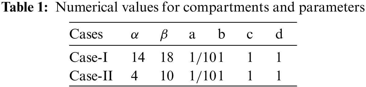
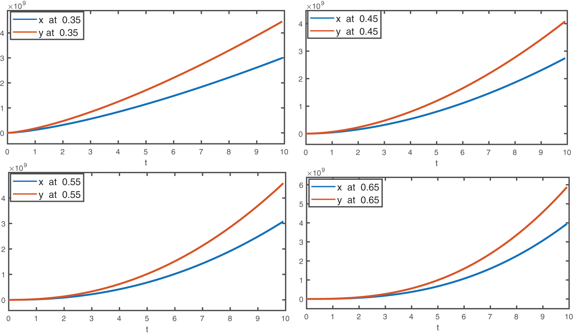
Figure 1: The graphical presentation of the first four terms approximates solutions for the considered model by using different values of fractional order as
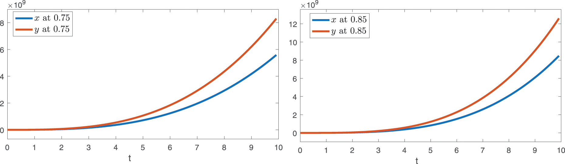
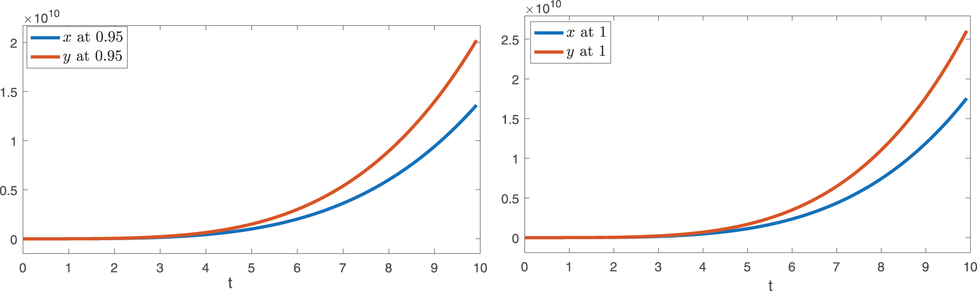
Figure 2: The graphical presentation of the first four terms approximates solutions for the considered model by using different values of fractional order as
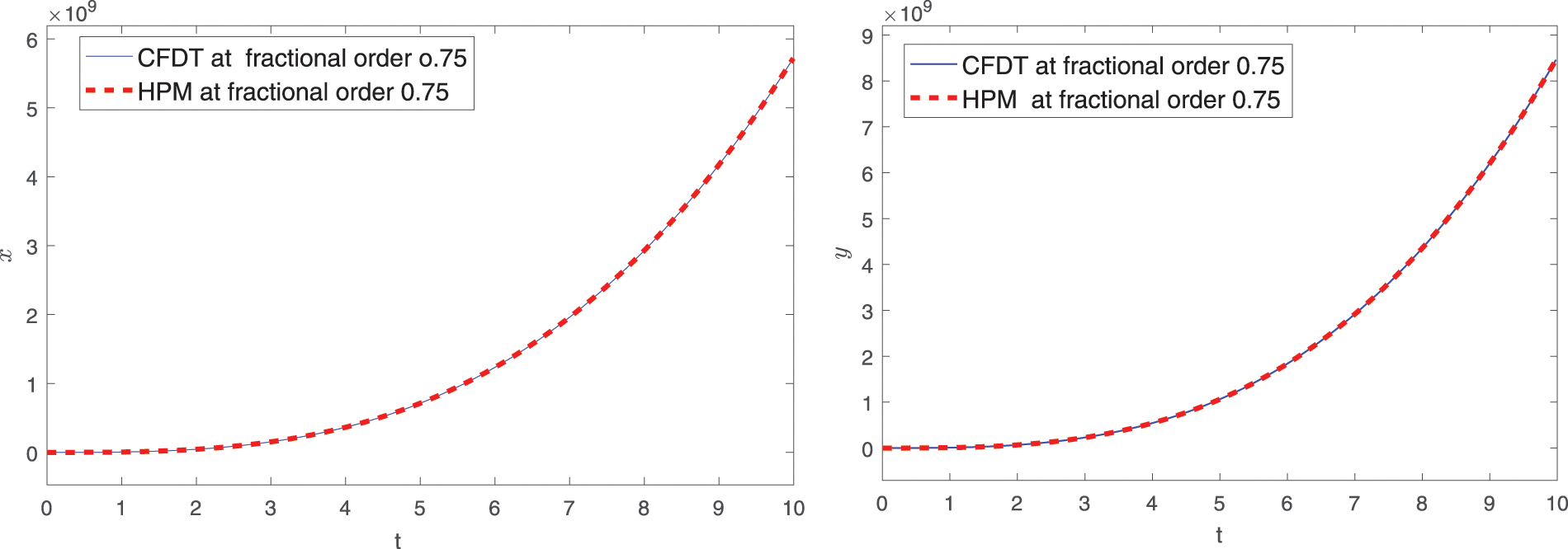
Figure 3: Comparison of solution of CFOD with that obtained by HPM under Caputo derivative at
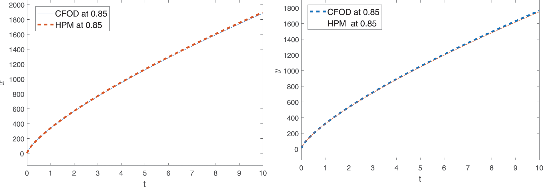
Figure 4: Comparison of solution of CFOD with that obtained by HPM under Caputo derivative at
Example 2. Consider another example of population dynamical model for the COVID-19. The concerned model has formed by updating the pre-predator model (3) by incorporating the immigration rate as
here
where
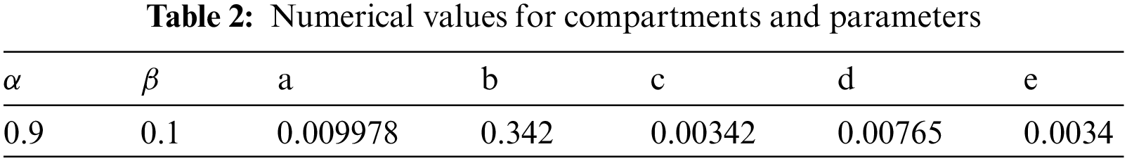
Here, now we use the following numerical value in the Table 2 in the system (25) to present graphically the first ten terms approximate solution of the model (24).
Now we present, the graphical presentation for initial ten terms for various fractional order in the following Figs. 5 and 6.
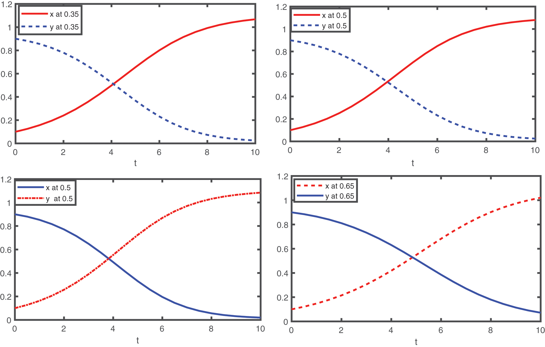
Figure 5: The graphical presentation of the first four terms approximates solutions for the considered model (23) by using different values of fractional order as

Figure 6: The graphical presentation of the first four terms approximates solutions for the considered model (23) by using different values of fractional order as
The interaction between susceptible class x and infected class y has shown in Figs. 5 and 6, by using two sets of fractional orders. In Fig. 5, we presented the approximate solution for first ten terms in case of susceptible and infected by taking the values of q as given by
This manuscript has been devoted to studying a nonlinear system under CFOD. The concerned dynamical system has been inspired by the famous prey-predator model of two species. For the problem under consideration, we have established some appropriate results for the existence and uniqueness of a solution by using the fixed point approach belonging to Banach and Schauder. Further, the CFDT technique has been applied to obtain the approximate solution to the considered system in the form of a series. By using computational software like Matlab, we have presented our results graphically for infinitely many terms using various values of fractional orders. We also compared our results to those obtained by HPM [62] for the Caputo derivative. We have observed that the solutions obtained by both methods behave nearly the same. Therefore, CFOD can also be exploited to study the dynamical behaviours of different real-world problems. Also, CFDT is a powerful tool like perturbation and decomposition methods to study various problems. But the interesting feature of CFDT is that it needs no extra control or prior correctional functions. Furthermore, it also needs no discretization of data and no collocation like Tau methods. The computation by using CFDT is easy to understand. In the future, we plan to apply the aforementioned technique to more complex dynamical systems, such as infectious disease models and neural network systems.
Acknowledgement: The authors K. Shah and T. Abdeljawad would like to thank Prince Sultan University for the support through the TAS Research Lab.
Funding Statement: The authors received no specific funding for this study.
Conflicts of Interest: The authors declare that they have no conflicts of interest to report regarding the present study.
References
1. Magin, R. (2004). Fractional calculus in bioengineering. Part 1, Critical reviews in biomedical engineering, vol. 32, no. 1. New York: Begell House Publishers. [Google Scholar]
2. Kilbas, A. A., Srivastava, H. M., Trujillo, J. J. (2006). Theory and applications of fractional differential equations. In: North holland mathematics studies, vol. 204. Amsterdam: Elseveir. [Google Scholar]
3. Baleanu, D., Machado, J. A. T., Luo, A. C. (2011). Fractional dynamics and control. New York: Springer Science & Business Media. [Google Scholar]
4. Podlubny, I. (1999). Fractional differential equations. New York: Academic Press. [Google Scholar]
5. Hilfer, R. (2000). Applications of fractional calculus in physics. Singapore: World Scientific. [Google Scholar]
6. Gómez-Aguilar, J. F., Atangana, A., Morales-Delgado, V. F. (2017). Electrical circuits RC, LC, and RL described by atangana-baleanu fractional derivatives. International Journal of Circuit Theory and Applications, 45(11), 1514–1533. DOI 10.1002/cta.2348. [Google Scholar] [CrossRef]
7. Koca, I., Atangana, A. (2017). Solutions of Cattaneo-Hristov model of elastic heat diffusion with Caputo-Fabrizio and Atangana-Baleanu ractional derivatives. Thermal Science, 21, 2299–2305. DOI 10.2298/TSCI160209103K. [Google Scholar] [CrossRef]
8. Valério, D., Machado, J. T., Kiryakova, V. (2014). Some pioneers of the applications of fractional calculus. Fractional Calculus and Applied Analysis, 17(2), 552–578. DOI 10.2478/s13540-014-0185-1. [Google Scholar] [CrossRef]
9. Sun, H., Zhang, Y., Baleanu, D., Chen, W., Chen, Y. (2018). A new collection of real world applications of fractional calculus in science and engineering. Communications in Nonlinear Science and Numerical Simulation, 64, 213–231. DOI 10.1016/j.cnsns.2018.04.019. [Google Scholar] [CrossRef]
10. Debnath, L. (2003). Recent applications of fractional calculus to science and engineering. International Journal of Mathematics and Mathematical Sciences, 2003(54), 3413–3442. DOI 10.1155/S0161171203301486. [Google Scholar] [CrossRef]
11. Salahshour, S., Ahmadian, A., Ismail, F., Baleanu, D. (2017). A fractional derivative with non-singular kernel for interval-valued functions under uncertainty. Optik, 130, 273–286. DOI 10.1016/j.ijleo.2016.10.044. [Google Scholar] [CrossRef]
12. Salahshour, S., Ahmadian, A., Abbasbandy, S., Baleanu, D. (2018). M-Fractional derivative under interval uncertainty: Theory, properties and applications. Chaos, Solitons & Fractals, 117, 84–93. DOI 10.1016/j.chaos.2018.10.002. [Google Scholar] [CrossRef]
13. Salahshour, S., Ahmadian, A., Salimi, M., Ferrara, M., Baleanu, D. (2019). Asymptotic solutions of fractional interval differential equations with nonsingular kernel derivative. Chaos: An Interdisciplinary Journal of Nonlinear Science, 29(8), 083110. DOI 10.1063/1.5096022. [Google Scholar] [CrossRef]
14. Kumar, S., Nieto, J. J., Ahmad, B. (2022). Chebyshev spectral method for solving fuzzy fractional fredholm-volterra integro-differential equation. Mathematics and Computers in Simulation, 192, 501–513. DOI 10.1016/j.matcom.2021.09.017. [Google Scholar] [CrossRef]
15. Kumar, S., Zeidan, D. (2021). An efficient mittag-lefier kernel approach for time-fractional advection-reaction-diffusion equation. Applied Numerical Mathematics, 170, 190–207. DOI 10.1016/j.apnum.2021.07.025. [Google Scholar] [CrossRef]
16. Kumar, S. (2020). Numerical solution of fuzzy fractional diffusion equation by chebyshev spectral method. Numerical Methods for Partial Differential Equations, 2020, 1–19. DOI 10.1002/num.22650. [Google Scholar] [CrossRef]
17. Senol, M., Atpinar, S., Zararsiz, Z., Salahshour, S., Ahmadian, A. (2019). Approximate solution of time-fractional fuzzy partial differential equations. Computational and Applied Mathematics, 38(1), 1–18. DOI 10.1007/s40314-019-0796-6. [Google Scholar] [CrossRef]
18. Singh, J., Ahmadian, A., Rathore, S., Kumar, D., Baleanu, D. et al. (2021). An efficient computational approach for local fractional poisson equation in fractal media. Numerical Methods for Partial Differential Equations, 37(2), 1439–1448. DOI 10.1002/num.22589. [Google Scholar] [CrossRef]
19. Khalil, R., Al Horani, M., Yousef, A., Sababheh, M. (2014). A new definition of fractional derivative. Journal of Computational and Applied Mathematics, 264, 65–70. DOI 10.1016/j.cam.2014.01.002. [Google Scholar] [CrossRef]
20. Abdeljawad, T. (2015). On conformable fractional calculus. Journal of Computational and Applied Mathematics, 279, 57–66. DOI 10.1016/j.cam.2014.10.016. [Google Scholar] [CrossRef]
21. Eslami, M., Rezazadeh, H. (2016). The first integral method for Wu-Zhang system with conformable time-fractional derivative. Calcolo, 53(3), 475–485. DOI 10.1007/s10092-015-0158-8. [Google Scholar] [CrossRef]
22. Ünal, E., Gökdogan, A., Çelik, E. (2015). Solutions of sequential conformable fractional differential equations around an ordinary point and conformable fractional hermite differential equation. arXiv preprint arXiv:1503.05407. [Google Scholar]
23. Chung, W. S. (2015). Fractional newton mechanics with conformable fractional derivative. Journal of Computational and Applied Mathematics, 290, 150–158. DOI 10.1016/j.cam.2015.04.049. [Google Scholar] [CrossRef]
24. Zhong, W., Wang, L. (2018). Basic theory of initial value problems of conformable fractional differential equations. Advances in Difference Equations, 2018(1), 1–14. [Google Scholar]
25. Al-Refai, M., Abdeljawad, T. (2017). Fundamental results of conformable sturm-liouville eigenvalue problems. Complexity, 2017, 3720471. DOI 10.1155/2017/3720471. [Google Scholar] [CrossRef]
26. Balci, E., Öztürk, I., Kartal, S. (2019). Dynamical behaviour of fractional order tumor model with caputo and conformable fractional derivative. Chaos, Solitons & Fractals, 123, 43–51. DOI 10.1016/j.chaos.2019.03.032. [Google Scholar] [CrossRef]
27. Harir, A., Melliani, S., Chadli, L. S. (2020). Fuzzy generalized conformable fractional derivative. Advances in Fuzzy Systems, 2020. DOI 10.1155/2020/1954975. [Google Scholar] [CrossRef]
28. El-Ajou, A., Oqielat, M. A. N., Al-Zhour, Z., Kumar, S., Momani, S. (2019). Solitary solutions for time-fractional nonlinear dispersive PDEs in the sense of conformable fractional derivative. Chaos: An Interdisciplinary Journal of Nonlinear Science, 29(9), 093102. DOI 10.1063/1.5100234. [Google Scholar] [CrossRef]
29. Al-Mdallal, Q. M., Hajji, M. A., Abdeljawad, T. (2021). On the iterative methods for solving fractional initial value problems: New perspective. Journal of Fractional Calculus and Nonlinear Systems, 2(1), 76–81. DOI 10.48185/jfcns.v2i1.297. [Google Scholar] [CrossRef]
30. Valdes, J. E. N., Guzmán, P. M., Bittencurt, L. M. L. M. (2020). A note on the qualitative behavior of some nonlinear local improper conformable differential equations. Journal of Fractional Calculus and Nonlinear Systems, 1(1), 13–20. DOI 10.48185/jfcns.v1i1.48. [Google Scholar] [CrossRef]
31. Kumar, R., Jain, S. (2021). Time fractional generalized korteweg-de vries equation: Explicit series solutions and exact solutions. Journal of Fractional Calculus and Nonlinear Systems, 2(2), 62–77. DOI 10.48185/jfcns.v2i2.315. [Google Scholar] [CrossRef]
32. Younus, A., Asif, M., Atta, U., Bashir, T., Abdeljawad, T. (2021). Some fundamental results on fuzzy conformable differential calculus. Journal of Fractional Calculus and Nonlinear Systems, 2(2), 31–61. DOI 10.48185/jfcns.v2i2.341. [Google Scholar] [CrossRef]
33. Ali, A., Shah, K., Alrabaiah, H., Shah, Z., Rahman, G. et al. (2021). Computational modeling and theoretical analysis of nonlinear fractional order prey-predator system. Fractals, 29(1), 2150001. DOI 10.1142/S0218348X21500018. [Google Scholar] [CrossRef]
34. Duarte, F., Machado, J. A. (2002). Chaotic phenomena and fractional-order dynamics in the trajectory control of redundant manipulators. Nonlinear Dynamics, 29(1), 315–342. [Google Scholar]
35. Molyneux, D. H. (1997). Patterns of change in vector-borne diseases. Annals of Tropical Medicine & Parasitology, 91(7), 827–839. [Google Scholar]
36. Estabrook, G. F. (2004). Essential mathematical biology. New York. [Google Scholar]
37. El-Sayed, A. M. A., Rida, S. Z., Arafa, A. A. M. (2009). On the solutions of time-fractional bacterial chemotaxis in a diffusion gradient chamber. International Journal of Nonlinear Science, 7(4), 485–492. [Google Scholar]
38. Hassan, H. N., El-Tawil, M. A. (2011). A new technique of using homotopy analysis method for solving high-order nonlinear differential equations. Mathematical Methods in the Applied Sciences, 34(6), 728–742. DOI 10.1002/mma.1400. [Google Scholar] [CrossRef]
39. Atangana, A., Koca, I. (2016). Chaos in a simple nonlinear system with atangana-baleanu derivatives with fractional order. Chaos, Solitons & Fractals, 89, 447–454. DOI 10.1016/j.chaos.2016.02.012. [Google Scholar] [CrossRef]
40. Liao, S. J. (2003). Beyond perturbation: Introduction to the homotopy analysis method. Boca Raton: Chapman Hall/CRC Press. [Google Scholar]
41. Rafei, M., Ganji, D. D., Daniali, H. (2007). Solution of the epidemic model by homotopy perturbation method. Applied Mathematics and Computation, 187(2), 1056–1062. DOI 10.1016/j.amc.2006.09.019. [Google Scholar] [CrossRef]
42. Awawdeh, F., Adawi, A., Mustafa, Z. (2009). Solutions of the SIR models of epidemics using HAM. Chaos, Solitons & Fractals, 42(5), 3047–3052. DOI 10.1016/j.chaos.2009.04.012. [Google Scholar] [CrossRef]
43. Rida, S. Z., Abdel Rady, A. S., Arafa, A. A. M., Khalil, M. (2012). Approximate analytical solution of the fractional epidemic model. International Journal of Applied Mathematical Research, 1(1), 17–29. DOI 10.14419/ijamr.v1i1.20. [Google Scholar] [CrossRef]
44. Arqub, O. A., El-Ajou, A. (2013). Solution of the fractional epidemic model by homotopy analysis method. Journal of King Saud University-Science, 25(1), 73–81. DOI 10.1016/j.jksus.2012.01.003. [Google Scholar] [CrossRef]
45. Rida, S. Z., Arafa, A. A. M., Gaber, Y. A. (2016). Solution of the fractional epidemic model by L-ADM. Journal of Fractional Calculus and Applications, 7(1), 189–195. [Google Scholar]
46. Biazar, J. (2006). Solution of the epidemic model by adomian decomposition method. Applied Mathematics and Computation, 173(2), 1101–1106. DOI 10.1016/j.amc.2005.04.036. [Google Scholar] [CrossRef]
47. Yousef, H. M., Ismail, A. M. (2018). Application of the laplace adomian decomposition method for solution system of delay differential equations with initial value problem. AIP Conference Proceedings, 020038. New York: AIP Publishing LLC. [Google Scholar]
48. Thieme, H. R. (1992). Convergence results and a poincaré-bendixson trichotomy for asymptotically autonomous differential equations. Journal of Mathematical Biology, 30(7), 755–763. DOI 10.1007/BF00173267. [Google Scholar] [CrossRef]
49. Abdelrazec, A. (2008). Adomian decomposition method: Convergence analysis and numerical approximations (M.Sc. Dissertation). McMaster University Hamilton, Canada. [Google Scholar]
50. Zhou, J. K. (1986). Differential transformation and its applications for electrical circuits. Wuhan, China: Huazhong University Press. [Google Scholar]
51. Ayaz, F. (2004). Solutions of the systems of differential equations by differential transform method. Applied Mathematics and Computation, 147, 547–567. [Google Scholar]
52. Hassan, I. H. (2008). Application to differential transformation method for solving systems of differential equations. Applied Mathematical Modelling, 32(12), 2552–2559. DOI 10.1016/j.apm.2007.09.025. [Google Scholar] [CrossRef]
53. Farshid, M. (2011). Differential transform method for solving linear and nonlinear systems of ordinary differential equations. Applied Mathematical Sciences, 5(70), 3465–3472. [Google Scholar]
54. Abdeljawad, T., Horani, A. L., Khalil, M. R. (2015). Conformable fractional semigroups of operators. Journal of Semigroup Theory and Applications, 2015. [Google Scholar]
55. Batarfi, H., Losada, J., Nieto, J. J., Shammakh, W. (2015). Three-point boundary value problems for conformable fractional differential equations. Journal of Function Spaces, 2015, 706383. DOI 10.1155/2015/706383 [Google Scholar] [CrossRef]
56. Dong, X., Bai, Z., Zhang, W. (2016). Positive solutions for nonlinear eigenvalue problems with conformable fractional differential derivatives. Journal of Shandong University of Science and Technology (Natural Science), 35, 85–90. [Google Scholar]
57. Das, S., Gupta, P. K. (2011). A mathematical model on fractional lotka-volterra equations. Journal of Theoretical Biology, 277, 1–6. DOI 10.1016/j.jtbi.2011.01.034. [Google Scholar] [CrossRef]
58. Pescitelli, M. (2013). Master dissertation lotka volterra predator-prey model with a predating scavenger. Georgia College. [Google Scholar]
59. O’Regan, D., Meehan, M. (2012). Existence theory for nonlinear integral and integrodifferential equations. New York: Springer Science & Business Media. [Google Scholar]
60. Johansson-Stenman, O. (1998). The importance of ethics in environmental economics with a focus on existence values. Environmental and Resource Economics, 11(3), 429–442. [Google Scholar]
61. Ünal, E., Gökdogan, A. (2017). Solution of conformable fractional ordinary differential equations via differential transform method. Optik, 128, 264–273. DOI 10.1016/j.ijleo.2016.10.031. [Google Scholar] [CrossRef]
62. Rafei, M., Daniali, H., Ganji, D. D. (2007). Variational iteration method for solving the epidemic model and the prey and predator problem. Applied Mathematics and Computation, 186(2), 1701–1709. DOI 10.1016/j.amc.2006.08.077. [Google Scholar] [CrossRef]
63. Shah, K., Khalil, H., Khan, R. A. (2018). Analytical solutions of fractional order diffusion equations by natural transform method. Iranian Journal of Science and Technology, Transactions A: Science, 42(3), 1479–1490. DOI 10.1007/s40995-016-0136-2. [Google Scholar] [CrossRef]
64. Leah, E. (2005). Mathematical models in biology. Philadelphia: Society for Industrial and Applied Mathematics. [Google Scholar]
65. Abdeljawad, T., Younus, A., Alqudah, M. A., Atta, U. (2023). On fuzzy conformable double laplace transform with applications to partial differential equations. Computer Modeling in Engineering & Sciences, 134(3), 2163–2191. DOI 10.32604/cmes.2022.020915. [Google Scholar] [CrossRef]
66. Elshenhab, A. M., Wang, X., Mofarreh, F., Bazighifan, O. (2023). Exact solutions and finite time stability of linear conformable fractional systems with pure delay. Computer Modeling in Engineering & Sciences, 134(2), 927–940. DOI 10.32604/cmes.2022.021512. [Google Scholar] [CrossRef]
67. Turkyilmazoglu, M. (2021). Nonlinear problems via a convergence accelerated decomposition method of adomian. Computer Modeling in Engineering & Sciences, 127(1), 1–22. DOI 10.32604/cmes.2021.012595. [Google Scholar] [CrossRef]
68. Shah, K., Abdeljawad, T., Mahariq, I., Jarad, F. (2020). Qualitative analysis of a mathematical model in the time of COVID-19. BioMed Research International, 2020, 5098598. DOI 10.1155/2020/5098598. [Google Scholar] [CrossRef]
Cite This Article
 Copyright © 2023 The Author(s). Published by Tech Science Press.
This work is licensed under a Creative Commons Attribution 4.0 International License , which permits unrestricted use, distribution, and reproduction in any medium, provided the original work is properly cited.
 Downloads
 Citation Tools