
 Submit a Paper
 Propose a Special lssue
 Open Access
ARTICLE

Temperature Field in Laser Line Scanning Thermography: Analytical Calculation and Experiment
1
China Aerodynamics Research and Development Center, Mianyang, 621000, China
2
Xi’an Research Institute of High Technology, Xi’an, 710025, China
3
Nanjing Novelteq, Ltd., Nanjing, 210038, China
* Corresponding Author: Bowen Liu. Email:
(This article belongs to the Special Issue: Advanced Computational Models for Decision-Making of Complex Systems in Engineering)
Computer Modeling in Engineering & Sciences 2023, 137(1), 1001-1018. https://doi.org/10.32604/cmes.2023.027072
Received 12 October 2022; Accepted 14 December 2022; Issue published 23 April 2023
 View Full Text
 Download PDF
Abstract
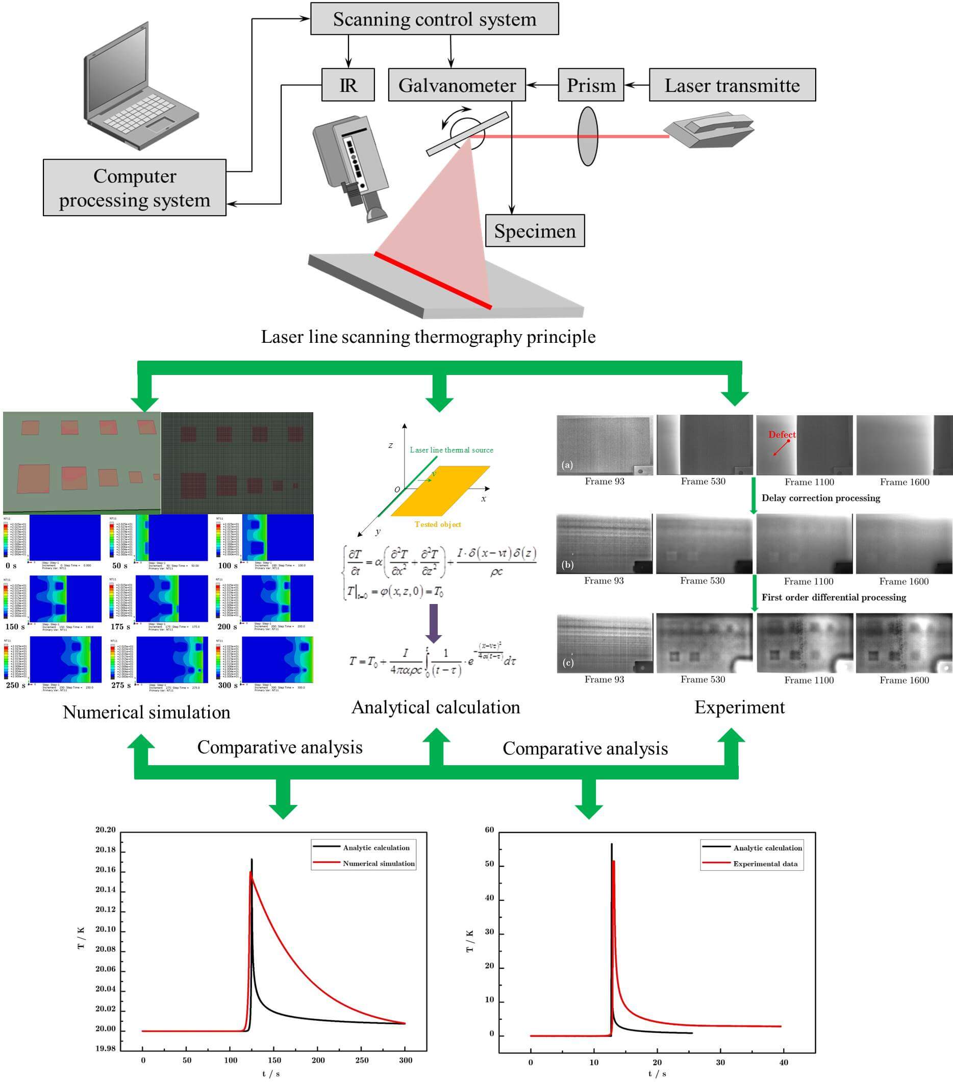
The temperature field in laser line scanning thermography is investigated comprehensively in this work, including analytical calculation and experiment. Firstly, the principle of laser line scanning thermography is analyzed. On this basis, a physical laser line scanning model is proposed. Afterwards, based on Fourier transform (FT) and segregation variable method (SVM), the heat conduction differential equation in laser line scanning thermography is derived in detail. The temperature field of the composite-based coatings model with defects is simulated numerically. The results show that the laser line scanning thermography can effectively detect the defects in the model. The correctness of the analytical calculation is verified by comparing the surface temperature distribution obtained by analytical calculation and numerical simulation. Additionally, an experiment is carried out and the changeable surface temperature obtained by analytical calculation is compared with the experimental results. It shows that the error of maximum temperature obtained by analytical calculation and by experiment is 8% with high accuracy, which proves the correctness of analytical calculation and enriches the theoretical foundation of laser line scanning thermography.Graphic Abstract
Keywords
Nomenclature
| I | Stimulation power |
| α | Heat diffusion coefficient |
| ρ | Density |
| c | Specific heat |
| δ( ) | Impulse function |
| v | Scanning velocity |
| T0 | Initial temperature |
| Q | Combined power parameter |
| e | Natural logarithm |
| R | Light source radius |
Nowadays, amounts of non-destructive testing (NDT) techniques are investigated for detecting metals, composites, and ceramics, such as ultrasonic testing, magnetic particle testing, eddy current, radiography, penetration, acoustic emission, microwave, shearography, and infrared thermography. Among them, the infrared thermography attracts extensive attention in the world due to its advantages of high-speed, high-resolution, full-field, and intuitional results in NDT [1–3]. For different defects in the materials, various thermal stimulation sources have been developed, which are mainly comprised of vibrothermography, induction thermography, and optical thermography [4]. The vibrothermography [5], also known as ultrasound infrared thermography, is sensitive to cracks and possesses the advantages of defect selective imaging and good adaptability to complex geometric measurements. But it is a contact NDT technology and needs to hold the tested object, which may burn the tested object. The induction thermography consists of eddy current thermography and microwave thermography [6,7], which have good detectability for the defects through appropriate algorithms. But the eddy current thermography cannot detect the non-conductive materials and deeper defects in the tested object due to the skin effect, and the microwave thermography cannot effectively stimulate the metals due to the metal interfaces reflection. Compared with the vibrothermography and induction thermography, the optical thermography is relatively simple and widely used, including pulsed thermography and laser thermography [8,9]. Optical thermography generally uses planar thermal stimulation sources, such as quartz lamps or flash lamps to stimulate the tested object. However, it is inevitable to produce afterglow effects that have a strong impact on the test results [10]. On this account, the laser line scanning thermography may be of great use because it can solve the problem of afterglow effects [11].
The theory of laser line scanning thermography is based on heat conduction. For heat conduction, Tamma et al. [12] utilized three-dimensional elements to investigate the heat conduction of the unidirectional composite materials based on the finite element method, but the built calculation model cost abundant of time due to the limitation of calculation method. To solve this problem, Savoia et al. [13] utilized an analytical method to study the heat conduction of the composites, but it was difficult for engineering application because of the limitation of boundary condition. Thus, to simplify the heat conduction function to guide the engineering applications, the one-dimensional heat conduction differential equation (similar to that used in traditional flash method proposed by Parker et al. [14]) can be used to analyze the heat conduction during pulsed thermography. Subsequently, Maldague et al. [15] assumed that the measured object was a semi-infinite homogeneous isotropic plate, and proposed that the three-dimensional differential equation of heat conduction could be simplified into a one-dimensional differential equation of heat conduction. Avdelidis et al. [16] established the numerical calculation model and investigated the feasibility of inspection of aircraft structures. The obtained results showed that the pulsed thermography could detect a subsurface defect and provide location information of the defect. However, with rapid development and engineering applications of advanced composite materials with anisotropic and inhomogeneous characteristics, scholars started to investigate the multi-dimensional heat conduction to facilitate the use of pulsed thermography for nondestructive testing of these advanced composite materials. Ozisik et al. [17,18] pointed out that the anisotropic domain could be transformed into isotropic domain through coordinate transformation. On this basis, Manohar et al. [19] proposed a virtual heat source model for rectangular defects. They analytically solved the three-dimensional heat conduction differential equations based on coordinate transformation and isolated variable method, which laid the foundation for quantitative evaluation of defects using pulsed thermography.
Unlike pulsed thermography, relative motion exists in laser line scanning thermography NDT. Therefore, heat conduction in laser line scanning thermography exists not only in the thickness direction, but also in the transverse direction, which is more complex than that in pulsed thermography. In allusion to the heat conduction in laser line scanning thermography, previous works mainly focused on the numerical study [11,20–24] but did not involve the theoretical and analytical solution. On this account, this work focuses on the heat conduction in laser line scanning thermography and attempts to solve the analytical solution of temperature field in laser line scanning thermography, which can enrich the theoretical foundation of laser line scanning thermography.
In the present paper, the temperature field in laser line scanning thermography is comprehensively investigated including analytical calculation, numerical simulation and experiment. In the subsequent sections, the laser line scanning thermography principle was described and a physical laser line scanning model is proposed. On this basis, an analytical solution was first derived in detail to represent the surface temperature followed by a numerical calculation to enrich the theoretical foundation of laser line scanning thermography. Finally, an experiment was carried out to validate the analytical solution.
2 Analytical Calculations on Temperature Field
2.1 Detection Principle of Laser Line Scanning Thermography
Laser line scanning thermography is an active NDT technology and its detection principle is shown in Fig. 1 [25]. The laser beam emitted by the laser transmitte passes through the prism to form a laser line. The laser line is reflected by a galvanometer to stimulate the tested specimen with a certain velocity, which is controlled by scanning control system. If defects exist in the tested specimen, a difference in surface temperature will be generated due to the electrical conductivity difference deviation between the sound region and the defect region, which can be gathered by an infrared camera. The defects in the tested specimen can be quantitatively evaluated by analyzing the thermal image sequence containing the defect information.
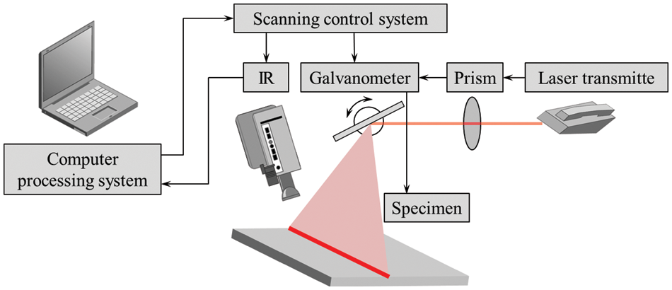
Figure 1: Laser line scanning thermography principle [25]
2.2 Derivation on Surface Temperature
According to the above description of the laser line scanning thermography principle, the theoretical essence of laser line scanning thermography is to solve the heat conduction differential equation under the stimulation of a moving line heat source. Different from pulsed thermography, in which the heat conduction differential equation is shown as Eq. (1) by assuming the tested object as a half infinite homogeneous and isotropy plate, there exists a relative movement in laser line scanning thermography NDT. As a result, the heat conduction in laser line scanning thermography exists not only in the thickness direction, but also in the transverse direction, which is more complex than that in pulsed thermography.
A physical model regarding to laser line scanning process is established as shown in Fig. 2, in which the tested object is placed at xOy plane and vertical to z-axis. The tested object is scanned by laser line thermal source along the x-axis with the velocity of v. The heat conduction mainly focuses on the x-axis direction and z-axis direction. Thus, the laser line thermal source can be illuminated as shown in Eq. (2) and the heat conduction differential equation under laser line scanning can be described by Eq. (3).
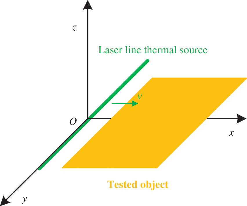
Figure 2: Laser line scanning physical model
In Eqs. (2) and (3), I is the stimulation power, α is the heat diffusion coefficient, ρ is the density, c is the specific heat,
Setting
In fact, Eq. (4) is the standard form of the Cauchy question for heat conduction equation, which can be solved based on FT and SVM.
According to the derivation principle for FT, processing the Eq. (4) with FT yields
The solution of Eq. (5) can be obtained based on SVM as shown in Eq. (6), which is validated in Appendix A.
Processing the Eq. (6) with inverse FT yields
According to the initial condition of
So,
By letting
Similarly,
Due to
Thus the analytical solution of Eq. (3) is
Generally, in laser line scanning thermography, the surface temperature of tested object is gathered by infrared camera. By letting z = 0, the surface temperature is
Eq. (17) represents the surface temperature of the tested specimen that is stimulated by laser line scanning, which is influenced by laser scanning parameters (stimulation power I and scanning velocity v) and material properties of tested specimen (heat diffusion coefficient α, density ρ and specific heat c). Thus, for a given tested specimen and laser scanning parameters, the corresponding surface temperature T can be obtained by Eq. (17).
3 Comparison between Numerical Simulation and Analytical Calculation
In the present section, numerical simulation is investigated to validate the correctness of analytical calculation. The multi-layer structure widely used in aircraft, rockets, and hypersonic vehicles [26,27] is employed as thermal protective structures and coating structures to calculate the surface temperature field.
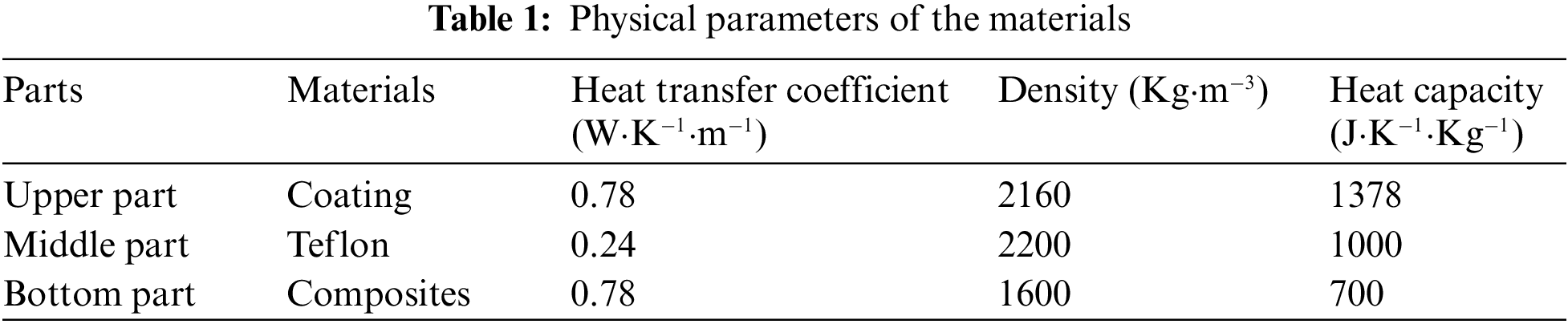
The temperature field of composite-based coatings with/without interfacial de-bonding defects is calculated in this section when the surface is scanned by the line laser at constant speed. As shown in Fig. 3, the composite-based coatings model consists of upper, middle and bottom parts. The upper part represents the coating, with the diameters of 150 × 100 × 0.2 mm3. The bottom part is the substrate, which is composed of composite material with the size of 150 × 100 × 4 mm3. The middle parts are the de-bonding defects, which are simulated by teflons with different sizes and arrangements to better simulate the diverse heat conduction process. As shown in Fig. 4, the teflons are arranged in upper and lower two rows with a thickness of 0.3 mm in the Y direction. In the upper row, four teflons with the sizes of 15 × 15 mm2 are uniformed arranged at 20 mm apart in the X direction to simulate uniform distribution of defects. In the lower row, five teflons gradually decrease in size from left to right. In detail, the maximum size of teflon is 25 × 25 mm2 with a gradient of 5 × 5 mm2, and the minimum size is 5 × 5 mm2. These teflons are similarly uniformed arranged at 10 mm apart in the X direction. It is worth noting that in the upper left figure in Fig. 3, the upper surface part is transparent in order to clearly indicate the position of the defects. Table 1 shows the physical parameters of the calculated materials [28].
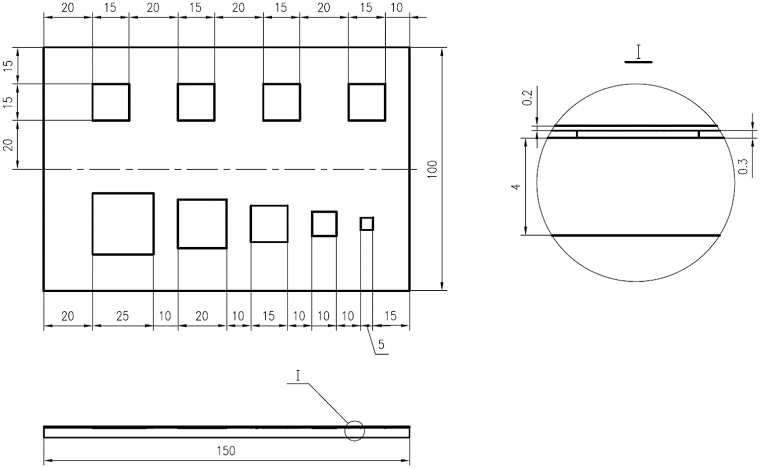
Figure 3: The position and size of composite-based coatings model
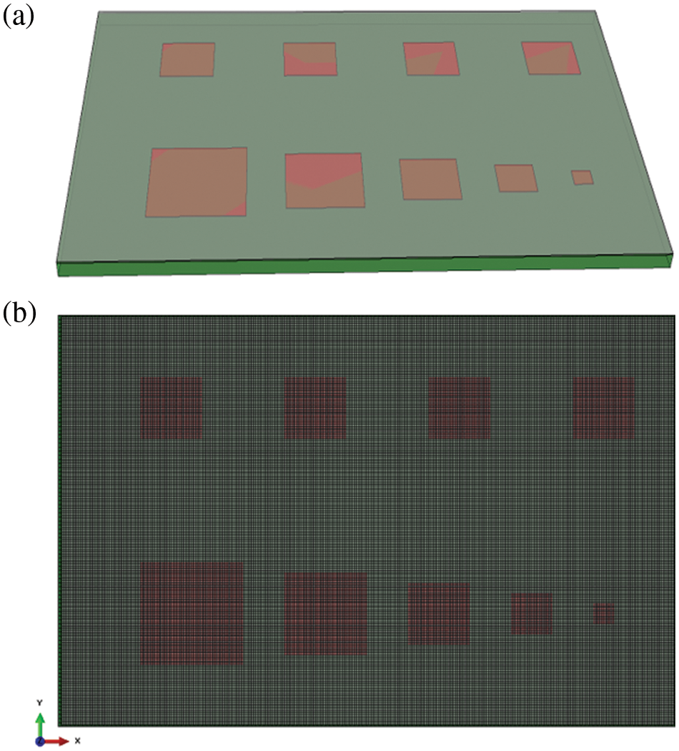
Figure 4: The geometric model and FEM model
The laser heat source is scanned from left to right on the surface of coating. The laser heat source belongs to Gaussian heat source. Its body heat source formula is shown in Eq. (18a). In this work, the formula degenerated into plane strip is shown as Eq. (18b).
where Q is the combined power parameter, e is the natural logarithm and R represents the light source radius.
In order to calculate the surface temperature field of the composite-based coatings model, the commercial software ABAQUS is used to implement the above calculation process. During the calculation process, the stimulation parameters are set, such as scanning speed of 0.5 mm/s, laser power of 100 W, laser beam width of 0.4 mm. Additionally, the initial temperature field and the convection heat exchange coefficient are set as 20 K and 10 W/(m2·K), respectively. It is noteworthy that not all nodes are scanned for 100 W in the numerical simulation. In fact, the sum of power of all simulated nodes is 100 W, that is, the laser scanning power of each node is 100 W divided by the number of nodes.
The post-processing module of ABAQUS is used to display the surface temperature thermographs of model at arbitrary scanning time. Meanwhile, for the accuracy of the calculation results, the mesh density needs to be adjusted according to the scanning rate, so as to ensure that the peak value of laser power falls on the element integration point at each calculation step and reflect the heat flow gradient. The geometric model and FEM model established by ABAQUS are shown in Fig. 4.
3.2 Numerical Simulation Results Analysis
The surface temperature field obtained by laser line scanning thermography is shown in Fig. 5.
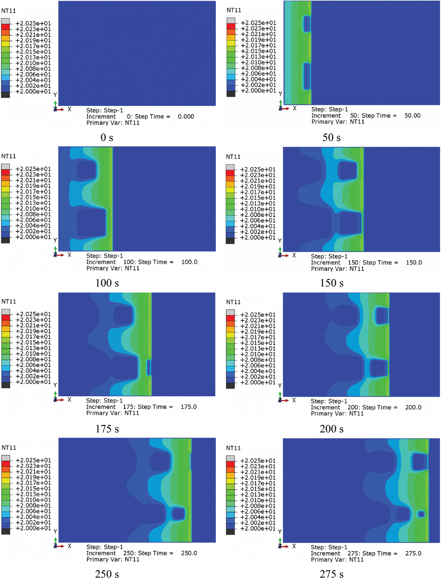

Figure 5: The surface temperature field obtained by laser line scanning thermography
In Fig. 5, the surface temperature heat maps of composite-based coatings at nine specific time points are collected at 0, 50, 100, 150, 175, 200, 250, 275 and 300 s, respectively. These time points correspond to the scanning time after laser scanning each internal defect. As the different heat conduction properties of the defective and non-defective regions, the corresponding surface temperature field can reveal the defects because of the temperature discontinuity in the calculation results. Fig. 5 shows the dynamic thermal image sequence regarding to the whole process of emergence, expansion and regression of defect hot spots in the model. At 0 s, the moving heat source has not scanned the defects, so no defect is detected. Therefore, the surface temperature of the model was 20 K, consistent with the initial temperature. At 50 s, the leftmost defects (1# and 5#) are scanned by heat source, and the surface temperature discontinuity occurs between the defect area and the sound area. At 100 s, the hot spots of defects 1# and 5# can be completely observed. As the heat source moving to the right, the hot spots of defects 2# and 6# are observed at 150 s. Meanwhile, due to the convection heat transfer between the model and surroundings, the hot spots of defects 1# and 5# are expanded or even regressed, resulting in the surface temperature of the defect area and the sound area gradually tend to balance until the defect hot spots disappear. The other defects in the model go through the whole process as well as the defects 1# and 5#. At 300 s all defects in the model are detected. It is worth noting that the surface temperature of the defect area is lower than that of the sound area. The reason is that the thermal conductivity of teflon used to simulate the de-bonding defect in the model is greater than that of air, and the corresponding thermal impedance is smaller than that of air, resulting in the heat accumulation in the defect area is less than that of the sound area.
In order to quantitatively characterize the variation of surface temperature in defective and acoustic regions under laser line scanning, the surface temperature history curves corresponding to the defect area and the sound area are analyzed. As shown in Fig. 6, the central points of the nine defects are numbered with 1#–9#, and the other nine points in the sound area located on the same vertical line and stimulated by moving heat source at the same time with 1#–9# are numbered with 1′#–9′#. The temperature history data of the above mentioned points are acquired and the corresponding curves of temperature vs. time are shown in Fig. 7.

Figure 6: The adopted points in defect and sound area

Figure 7: The temperature history curve of the adopted points. (a) 1#–4# and 1′#–4′#. (b) 5#–9# and 5′#–9′#
It can be seen from Fig. 7, the initial temperature is consistent with the room temperature of 20 K, since no point has been scanned. When the moving heat source scans to these adopted points, the corresponding temperature rises sharply. In detail, the temperature of 1′#–9′# is higher than that of 1#–9#, indicating that the surface temperature of the defect area is lower than that of the sound area, which is consistent with the analysis results of thermal image sequence. Afterwards, the temperature starts to decrease to room temperature under the action of air convection. It should be noted that the temperature at the points 1#–9# falls faster than that at the points 1′#–9′#, which indicates that the temperature of the defect area falls faster than that of the sound area due to the larger thermal conductivity of teflon. In addition, it can be seen from Fig. 7 that the temperature history of the points 1#–9# located at the center of the defect is consistent, and the temperature history of points 1′#–9′# in the sound area is also consistent, indicating that the defect size has a slight influence on the temperature of laser heat conduction. In order to compare with the analytical solution and the numerical simulation, the temperature history curve of point 2# on the model surface is obtained through analytical calculation and by numerical simulation, as shown in Fig. 8.

Figure 8: The surface changeable temperatures obtained by analytical calculation and by numerical simulation
As can be seen from Fig. 8, the surface temperature obtained through analytical solution and numerical simulation presents a manner of “stable-rise-decrease”. In the stable stage, the temperature of both points is 0 K, as they have not yet been scanned. In the rise stage, the curve obtained by analytical calculation is highly consistent with that obtained by numerical simulation. The maximum surface temperature obtained by the analytical calculation is 20.17 K, which is approximately equal to the 20.16 K obtained by the numerical simulation, thus verifying the correctness of the analytical calculation. In the decrease stage, the curve obtained by analytical calculation declines more rapidly than that obtained by numerical simulation, because the convective heat transfer coefficient is different, that is, the convective heat transfer coefficient is set as 10 in numerical calculation, while the convective heat transfer coefficient is neglected in analytical calculation, resulting in divergent descending speed.
The specimen studied in the work is made up of composite-based coatings with the substrate of composite material extended in [(0/−45/90/45)2/0/90]s and the coating of S04–80 mat enamel paint. In the specimen, 9 rectangular teflons are embedded to simulate the hole defects. The number and size of the 9 defects are consistent with those in the FEM model. The defects in the upper row are embedded at the depth of 0.5, 1, 2 and 3 mm, respectively, and those in the lower row are embedded at a depth of 2 mm. The specimen geometry is shown in Fig. 9.

Figure 9: The specimen geometry. (a) The composite material based substrate. (b) S04-80 mat enamel paint
The laser line scanning thermography detection device is shown in Fig. 10, including the laser line scanning stimulation system, computer processing system, computer screen, cooling system and mobile cabinet.
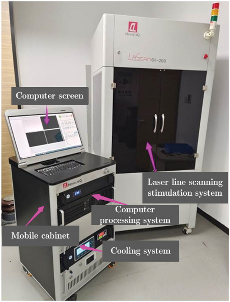
Figure 10: The laser line scanning device
The specimen was stimulated by a laser linear scanning stimulation system with a scanning power of 100 W and a linear scanning speed range of 0–50 mm/s. The computer processing system is applied to carry out thermal image sequence processing, and the cooling system is used to cool down the device. The FLIR X6530sc infrared camera is integrated with the laser linear scanning stimulation system to capture the thermal image sequence. It can measure a temperature range of 5°C to 150°C with a sensitivity of 20 mK at 25°C, and a maximum thermal image capture rate of 145 frames per second with a resolution of 640 × 512 pixels. In the process of laser line scanning thermography detection, the specimen is fastened by the clamp and scanned by the laser beam from left to right. The specimen is captured by infrared camera with the rate of 100 frames per second.
4.2 Experimental Results Analysis
The detection results of laser line scanning thermography are shown in Fig. 11. Some thermal images that can display the whole laser line scanning process are adopted under different frames.

Figure 11: The thermal image sequence of a specimen under different frames. (a) The original thermal image sequence. (b) The thermal image sequence processed by a delay correction algorithm. (c) The thermal image sequence processed by first order differential algorithm
From Fig. 11a, in frame 93, the specimen is not scanned yet by laser beam, resulting in no heat accumulation on the specimen surface. As the laser beam scanning proceeds, the defect 1# with a depth of 0.5 mm is dimly displayed in frame 1100 and faded in frame 1600, but other defects are not shown during the scanning process. Additionally, due to the delay effect in the thermal image sequence caused by laser scanning stimulation, the specimen surface cannot be stimulated simultaneously. Therefore, to visually observe the temperature field on the surface of the sample, a delay correction algorithm [29] integrated with the computer processing system is applied to process the thermal image sequence. The corresponding results are shown in Fig. 11b, where the delay effect is eliminated and more defects can be observed, but the defect contrast is relatively low. To obtain the high contrast, the first order differential algorithm is used to process the thermal image sequence. The corresponding results are shown in Fig. 11c, where most defects are clearly observed, but the defects 4# and 9# are still not observed. The reason for the defect 4# may be due to the interference of reflection of clamp, and the reason for the defect 9# may be due to its small size that exceeds the detection range.
In order to directly characterize the changeable temperature, the temperature curves of the defect region and the sound region are obtained as shown in Fig. 12. The curve corresponding to the defect area decreases more rapidly than that of the sound area, resulting in a discontinuity of temperature in the thermography sequence, which is consistent with the numerical calculation results. Differently, the temperature value obtained by experimental is larger than that obtained through numerical simulation, because the laser power in the experiment is 100 W, while in the numerical simulation, the laser scanning power of each node is 100 W divided by the number of nodes.
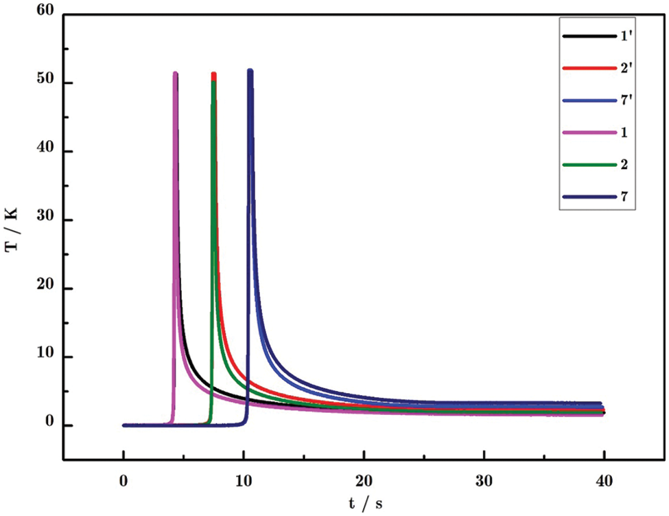
Figure 12: The temperature curve corresponding to the defect area and to the sound area
Fig. 13 shows the surface temperature obtained through analytical calculation and experiment. Both temperature curves change in a “stable-rise-decrease” manner. In the stable and rising stages, the two temperature curves are highly consistent. The maximum surface temperature calculated by analysis and measured by experiment are about 57 and 52 K, respectively, and the relative error between them is about 8%. However, in the decrease phase, the descent rates are different due to the air convection and complex environmental disturbance in the experiment.
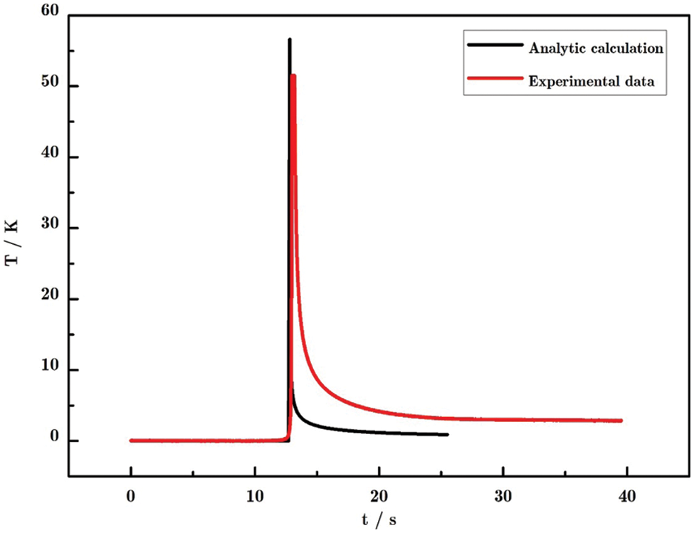
Figure 13: The surface changeable temperatures obtained by analytical calculation and by experiment
(1) A laser line scanning physical model is proposed according to the laser line scanning thermography detection principle. On this basis, the heat conduction differential equation under the stimulation of a moving line heat source is in detail derived based on FT and SVM, which lays the theoretical foundation for the laser line scanning thermography.
(2) A composite-based coatings model with defects is established to carry out the numerical simulation on surface temperature. The obtained results show that the laser line scanning thermography can detect the defects in the model. Additionally, the comparative analysis of the changeable surface temperature obtained by analytical calculation and by numerical simulation is studied. The maximum surface temperature obtained by analytical calculation is 20.17 K, which is approximately equal to 20.16 K obtained by numerical simulation, verifying the correctness of the analytical calculation.
(3) An experiment is carried out on composite-based coatings specimens. The experimental result shows that in combination with the thermal image sequence processing methods delay correction and first order differential algorithm, the defects in the specimen can be clearly detected using laser line scanning thermography. Additionally, the comparative analysis of the changeable surface temperature obtained by analytical calculation and by experiment is studied. The maximum surface temperature calculated by analysis and measured by experiment is about 57 and 52 K, respectively. The relative error between them is about 8%, which proves the correctness of the analytical calculation.
In summary, the temperature field under the laser line scanning stimulation is comprehensively investigated through analytical calculation and experiment in the present work, which enriches the theoretical foundation of laser line scanning thermography. Subsequently, considering the convection heat exchange coefficient, the analytical calculation will be continually investigated to better guide the numerical simulation and experiment.
Funding Statement: This work is supported by the National Natural Science Foundation of China (Grant No. 52005495).
Conflicts of Interest: The authors declare that they have no conflicts of interest to report regarding the present study.
References
1. Kher, V., Mulaveesala, R. (2020). Probability of defect detection in glass fibre reinforced polymers using pulse compression favourable frequency modulated thermal wave imaging. Infrared Physics & Technology, 113(9), 103616. https://doi.org/10.1016/j.infrared.2020.103616 [Google Scholar] [CrossRef]
2. Li, Y., Song, Y. (2021). A novel thermographic methodology to predict damage evolution of impacted CFRP laminates under compression-compression fatigue based on inverted Weibull model. IEEE Sensors Journal, 21(10), 11393–11400. https://doi.org/10.1109/JSEN.2020.2997458 [Google Scholar] [CrossRef]
3. Junyan, L., Liqiang, L., Yang, W. (2013). Experimental study on active infrared thermography as a NDI tool for carbon-carbon composites. Composites Part B: Engineering, 45(1), 138–147. https://doi.org/10.1016/j.compositesb.2012.09.006 [Google Scholar] [CrossRef]
4. Schweizer, S. (2022). Design and construction of an led-based excitation source for lock-in thermography. Applied Sciences, 12(6), 2940. https://doi.org/10.3390/app12062940 [Google Scholar] [CrossRef]
5. Yu, Q., Obeidat, O., Han, X. (2018). Ultrasound wave excitation in thermal NDE for defect detection. NDT & E International, 100(6), 153–165. https://doi.org/10.1016/j.ndteint.2018.09.009 [Google Scholar] [CrossRef]
6. Liu, Y., Tian, G., Gao, B., Lu, X., Li, H. et al. (2022). Depth quantification of rolling contact fatigue crack using skewness of eddy current pulsed thermography in stationary and scanning modes. NDT & E International, 128(1–2), 102630. https://doi.org/10.1016/j.ndteint.2022.102630 [Google Scholar] [CrossRef]
7. He, H., Zhao, Y., Lu, B., He, Y., Shen, G. et al. (2022). Detection of debonding defects between radar absorbing material and CFRP substrate by microwave thermography. IEEE Sensors Journal, 22(5), 4378–4385. https://doi.org/10.1109/JSEN.2022.3144827 [Google Scholar] [CrossRef]
8. Maldague, X. (2021). Data enhancement via low-rank matrix reconstruction in pulsed thermography for carbon-fibre-reinforced polymers. Sensors, 21(21), 7185. https://doi.org/10.3390/s21217185 [Google Scholar] [PubMed] [CrossRef]
9. Li, T., Almond, D. P., Rees, D. A. S. (2011). Crack imaging by scanning pulsed laser spot thermography. NDT & E International, 44(2), 216–225. https://doi.org/10.1016/j.ndteint.2010.08.006 [Google Scholar] [CrossRef]
10. Sun, J. G. (2006). Analysis of pulsed thermography method for defect depth prediction. Journal of Heat Transfer, 128(4), 329–338. https://doi.org/10.1115/1.2165211 [Google Scholar] [CrossRef]
11. Liu, Z., Jiao, D., Shi, W., Xie, H. (2017). Linear laser fast scanning thermography NDT for artificial disbond defects in thermal barrier coatings. Optics Express, 25(5), 31789–31800. https://doi.org/10.1364/OE.25.031789 [Google Scholar] [PubMed] [CrossRef]
12. Tamma, K. K., Yurko, A. A. (1988). A unified finite element modeling/analysis approach for thermal—structural response in layered composites. Computers & Structures, 29(5), 743–754. https://doi.org/10.1016/0045-7949(88)90342-2 [Google Scholar] [CrossRef]
13. Savoia, M., Reddy, J. N. (1995). Three-dimensional thermal analysis of laminated composite plates. International Journal of Solids Structures, 32(5), 593–608. https://doi.org/10.1016/0020-7683(94)00146-N [Google Scholar] [CrossRef]
14. Parker, W. J., Jenkins, R. J., Butler, C. P., Abbott, G. L. (1961). Flash method of determining thermal diffusivity, heat capacity and thermal conductivity. Journal of Applied Physics, 32(9), 1679–1684. https://doi.org/10.1063/1.1728417 [Google Scholar] [CrossRef]
15. Maldague, X. (2001). Theory and practice of infrared technology for nondestructive testing. New York: John Wiley Interscience. [Google Scholar]
16. Avdelidis, N. P., Almond, D. P. (2004). Transient thermography as a through skin imaging technique for aircraft assembly: Modeling and experimental results. Infrared Physics & Technology, 45(2), 103–114. https://doi.org/10.1016/j.infrared.2003.07.002 [Google Scholar] [CrossRef]
17. Ozisik, M. N. (1979). Heat conduction. New York: Wiley-Interscience Publication. [Google Scholar]
18. Carslaw, H. S., Jaeger, J. C. (1959). Conduction of heat in solids. London: Oxford Science Publications. [Google Scholar]
19. Manohar, A., Scalea, F. L. D. (2014). Modeling 3D heat flow interaction with defects in composite materials for infrared thermography. NDT & E International, 66(5), 1–7. https://doi.org/10.1016/j.ndteint.2014.04.003 [Google Scholar] [CrossRef]
20. Xu, Y., Hwang, S., Wang, Q., Kim, D., Luo, C. et al. (2020). Laser active thermography for debonding detection in FRP retrofitted concrete structures. NDT & E International, 114(4), 102285. https://doi.org/10.1016/j.ndteint.2020.102285 [Google Scholar] [CrossRef]
21. Puthiyaveettil, N., Thomas, K. R., Unnikrishnakurup, S., Myrach, P., Ziegler, M. et al. (2020). Laser line scanning thermography for surface breaking crack detection: Modeling and experimental study. Infrared Physics & Technology, 104(5), 103141. https://doi.org/10.1016/j.infrared.2019.103141 [Google Scholar] [CrossRef]
22. Jiao, D., Shi, W., Liu, Z., Xie, H. (2018). Laser multi-mode scanning thermography method for fast inspection of micro-cracks in TBCs surface. Journal of Nondestructive Evaluation, 37(2), 30. https://doi.org/10.1007/s10921-018-0485-1 [Google Scholar] [CrossRef]
23. Liu, H., Du, W., Nezhad, H. Y., Starr, A., Zhao, Y. (2021). A dissection and enhancement technique for combined damage characterisation in composite laminates using laser-line scanning thermography. Composite Structures, 271(12), 114168. https://doi.org/10.1016/j.compstruct.2021.114168 [Google Scholar] [CrossRef]
24. Qiu, J., Pei, C., Yang, Y., Wang, R., Liu, H. et al. (2021). Remote measurement and shape reconstruction of surface-breaking fatigue cracks by laser-line thermography. International Journal of Fatigue, 142(5), 105950. https://doi.org/10.1016/j.ijfatigue.2020.105950 [Google Scholar] [CrossRef]
25. Li, Y., Song, Y., Yang, Z., Xie, X. (2022). Use of line laser scanning thermography for the defect detection and evaluation of composite material. Science and Engineering of Composite Materials, 29(1), 74–83. https://doi.org/10.1515/secm-2022-0007 [Google Scholar] [CrossRef]
26. Triantou, K., Mergia, K., Florez, S. (2015). Thermo-mechanical performance of an ablative/ceramic composite hybrid thermal protection structure for re-entry applications. Composites Part B: Engineering, 82(4), 159–165. https://doi.org/10.1016/j.compositesb.2015.07.020 [Google Scholar] [CrossRef]
27. Delfini, A., Pastore, R., Santoni, F. (2021). Thermal analysis of advanced plate structures based on ceramic coating on carbon/carbon substrates for aerospace Re-Entry Re-Useable systems. Acta Astronautica, 183, 153–161. https://doi.org/10.1016/j.actaastro.2021.03.013 [Google Scholar] [CrossRef]
28. Li, Y., Zhang, W., Yang, Z., Zhang, J., Tao, S. (2016). Low-velocity impact damage characterization of carbon fiber reinforced polymer (CFRP) using infrared thermography. Infrared Physics & Technology, 76(3), 91–102. https://doi.org/10.1016/j.infrared.2016.01.019 [Google Scholar] [CrossRef]
29. Jiang, H., Chen, L., Zhang, S. (2014). Application of the laser scanning infrared thermography for nondestructive testing. Nondestructive Testing, 36(12), 20–22. [Google Scholar]
Differentiating the Eq. (6) with respect to t yields
In order to simplify the calculation, by letting
Substituting
Additionally, letting
Thus, the Eq. (6) is validated as the analytical solution of Eq. (5).
Cite This Article
 Copyright © 2023 The Author(s). Published by Tech Science Press.
This work is licensed under a Creative Commons Attribution 4.0 International License , which permits unrestricted use, distribution, and reproduction in any medium, provided the original work is properly cited.
 Downloads
 Citation Tools