
 Submit a Paper
 Propose a Special lssue
 Open Access
ARTICLE

A Modified Principal Component Analysis Method for Honeycomb Sandwich Panel Debonding Recognition Based on Distributed Optical Fiber Sensing Signals
1 State Key Laboratory of Structural Analysis for Industrial Equipment, Dalian University of Technology, Dalian, 116024, China
2 Beijing Aerospace Technology Institution, Beijing, 116024, China
3 College of Water-Conservancy and Civil Engineering, Shandong Agricultural University, Taian, 271000, China
* Corresponding Author: Zhanjun Wu. Email:
Structural Durability & Health Monitoring 2024, 18(2), 125-141. https://doi.org/10.32604/sdhm.2024.042594
Received 05 June 2023; Accepted 28 November 2023; Issue published 22 March 2024
 View Full Text
 Download PDF
Abstract
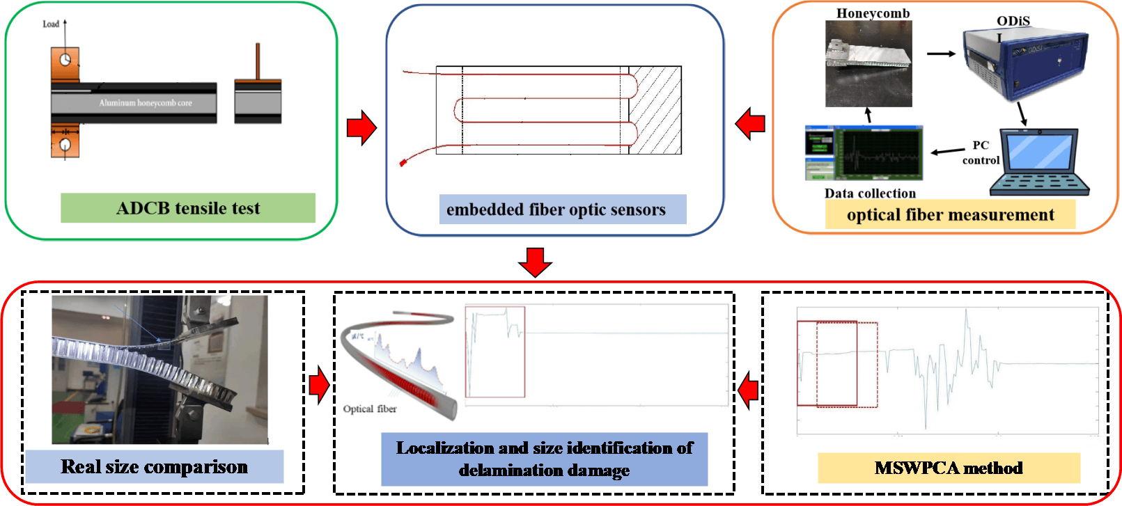
The safety and integrity requirements of aerospace composite structures necessitate real-time health monitoring throughout their service life. To this end, distributed optical fiber sensors utilizing back Rayleigh scattering have been extensively deployed in structural health monitoring due to their advantages, such as lightweight and ease of embedding. However, identifying the precise location of damage from the optical fiber signals remains a critical challenge. In this paper, a novel approach which namely Modified Sliding Window Principal Component Analysis (MSWPCA) was proposed to facilitate automatic damage identification and localization via distributed optical fiber sensors. The proposed method is able to extract signal characteristics interfered by measurement noise to improve the accuracy of damage detection. Specifically, we applied the MSWPCA method to monitor and analyze the debonding propagation process in honeycomb sandwich panel structures. Our findings demonstrate that the training model exhibits high precision in detecting the location and size of honeycomb debonding, thereby facilitating reliable and efficient online assessment of the structural health state.Graphic Abstract
Keywords
Nomenclature
| P | Principal component matrix |
| R | Covariance matrix |
| T2 | Hotelling statistic |
| X | Strain monitoring data |
| Λ | Diagonal matrix |
| E | Mathematical expectations |
| μ | Mean value |
| σ | Standard deviation |
| a | Debonding size |
Structural safety and integrity are central requirements for various aerospace structures. However, the harsh service environment can cause degradation of structural performance due to the accumulation of damage such as cracks, delamination, and interfacial debonding. Therefore, it is vital to develop structural health monitoring technologies for online awareness of structural damage state [1]. Various strain sensor networks have been widely used for structural health monitoring. Traditional strain monitoring techniques normally rely on discrete sensing elements such as strain gauges, fiber brag gratings (FBG) [2,3], etc. However, these sensor networks suffer from drawbacks including restricted structural coverage and low damage sensitivity due to the low density of measurement locations [4]. Distributed optical fiber sensors, on the other hand, offer several notable benefits such as lightweight, immunity to electromagnetic interference, and ease of embedding [5,6]. Moreover, this sensor can perform high-density, continuous measurements of strain and temperature. In recent years, distributed optical fiber sensing techniques utilizing back Rayleigh scattering have undergone remarkable development, showing demonstrated capabilities in detecting small structural damage that are crucial in aerospace applications [7–9].
Conventional approaches in damage identification, relying on strain measurement data for example, largely rely on manual identification of damage features from sensor signals. The process can be complex and laborious, requiring significant human resources and time expenditures. In the context of distributed optical fiber data processing, in particular, several challenges arise due to the large amount of data, significant noise interference, and intricate data complexity. Therefore, it is crucial to develop an automated damage identification methodology that utilizes distributed optical fiber monitoring data to extract quantitative damage features from complex strain information.
Recent advances in machine learning techniques have led to the increased use of various approaches and technologies, such as Bayesian methods [10], genetic algorithms [11], and artificial neural networks [12], in the field of structural health monitoring. With the continued improvement of computing capabilities, deep learning methods have rapidly gained popularity. Convolutional neural networks (CNNs) are among the most widely used deep learning models, and have been applied to structural damage identification using dynamic data [13–17]. However, CNNs have certain limitations in the field of damage identification. For example, building a robust CNN model for identifying structural damage requires a large amount of training data. As a supervised learning method, CNN relies on fully labeled datasets, which can be prohibitively expensive to acquire for structural damage-related samples [18]. Moreover, overfitting risks may readily arise in instances of limited data volumes.
The principal component analysis (PCA) is a widely employed technique within the realm of multivariate statistical process control (MSPC), primarily utilized for process monitoring. This method is extensively applied in the field of structural health monitoring [19–22]. Rather than relying on an extensive modeling of anomalies, it employs the distinguishing features of data samples in normal conditions as a reference benchmark to ensure recognition accuracy. The major advantage of PCA lies in its ability to reduce a vast number of data variables into a small set of principal components (i.e., comprehensive variables or indicators). These reduced-dimensional comprehensive indices are formulated as linear combinations of the original data. In essence, the PCA integrates the underlying features of the data with similar characteristics in order to derive a dimensionality reduction index [23]. Thus, in dealing with voluminous and intricate strain data obtained from distributed optical fibers, adoption of PCA model can offer significant benefits. Furthermore, when compared to conventional statistical error interval model, the PCA is also advantageous in several aspects. For example, the Hotelling statistic T2 serves as a principal component anomaly indicator, which mathematically represents the Markov distance of the principal component points to the new coordinate system [24]. This approach reflects changes in the distribution trend of the data, rather than indicating alterations in individual variables that may appear abnormally. In the context of big data analysis, the integration of appropriate algorithms can mitigate erroneous outcomes that arise due to noise. While conventional PCA allow for detection of anomalous data points, they are insufficient in terms of precision and localization of such deviations. This impedes their effectiveness in quantifying structural damage information.
This paper presented a new approach for identifying and locating damage using distributed optical fiber sensors with high-density strain measurement points. The proposed technique, named Modified Sliding Window Principal Component Analysis (MSWPCA), uses a local measurement point component PCA model to accurately detect anomalous data points. Moreover, by integrating Hotelling statistical thresholds, the proposed method automatically identifies and localizes damage, improving precision and reducing false positives. To demonstrate the robustness of the proposed approach, MSWPCA method was employed to track debonding propagation in honeycomb sandwich panel structures, specifically in an asymmetric double cantilever beam (ADCB) tensile experiment. The embedded distributed optical fiber sensing data from the structural interface is a valuable source of model data that can be utilized to enhance the accuracy of PCA and damage identification.
2.1 Principal Component Analysis
Let
where R represents the covariance matrix, Λ represents the diagonal matrix composed of m eigenvalues [λ1, λ2,..., λn]. P= [p1, p2,… pn] represents a standard orthogonal matrix composed of m eigenvectors.
Consider the following linear transformation
where t is the principal component after the coordinate transformation of the original data.
For the purpose of monitoring data X in multivariable statistical process control, the Hotelling statistic T2 can be used in PCA monitoring models to assess whether the monitoring data is anomalous [27]. The Hotelling statistic T2 is expressed as
To ascertain the abnormality of the monitored system, it is imperative to establish an appropriate safety threshold
2.2 Calculation of Safety Threshold T2
Assuming a normal distribution for the model error sample
According to Eq. (4), it can be observed that the probability of surpassing the 3-Sigma confidence interval is a statistically minute event, with only a 0.27% likelihood. Consequently, if the error sample mean from an unknown service state sample surpasses this range, it is deemed to be abnormal and indicative of damage. As such, the quantile Z of a normal distribution α/2 can be utilized to establish an appropriate safety threshold.
In certain instances, data may deviate from a strictly normal distribution and its underlying distribution may be unknown. When simulating such data using a normal distribution, deviations will arise. In such cases, it is necessary to ascertain the data distribution function and subsequently derive the α quantile value. Kernel density estimation interpolation can be used to estimate the data distribution function. The structural safety threshold, denoted as
Nevertheless, it should be noted that although PCA can effectively determine the presence of anomalous data, its utility is limited in that it only provides a binary decision regarding the abnormality. In practical monitoring scenarios, it is imperative to not only indicate aberrations but also accurately identify their spatial location within the dataset.
2.3 MSWPCA and Damage Warning Mechanism
Given the continuous and densely-distributed nature of optical fiber sampling points, localized damage typically results in a small range of regional anomalies, whereas sparse single point anomalies are most likely caused by noise. To address this issue, this paper presents an innovative MSWPCA method. The strain data of the optical fiber is partitioned into w sub-regions using a sliding window, and the identification of anomalies is performed based on the detection of regions where the Hotelling statistic component exceeds the predetermined threshold. Specifically, assuming that s continuous optical fiber data represents a local area, and each sliding window advances by n optical fiber data with s < n, then the total number of areas divided into w = m/s.
For monitoring the sample matrix
In the context of a monitoring sample matrix
where
Hence, the initial monitoring sample matrix X is augmented w fold (w = m/s). Subsequently, w novel monitoring sample matrices
Based on the aforementioned techniques, the damage warning procedure is established as follows:
(1) Offline status:
Step 1: involves the installation of optical fiber on the structure intended for monitoring purposes, followed by the acquisition of strain data several times under varying health conditions. This data is then utilized as training data to apply a Modified PCA model, enabling more precise monitoring and analysis.
Step 2: the kernel density estimation method is employed to determine both the global structural safety threshold
(2) Online status
Step 1: involves data collection of the current monitoring sample, followed by the calculation of its T2 statistics.
Step 2: the overall safety threshold
The flow chart is shown in Fig. 1.
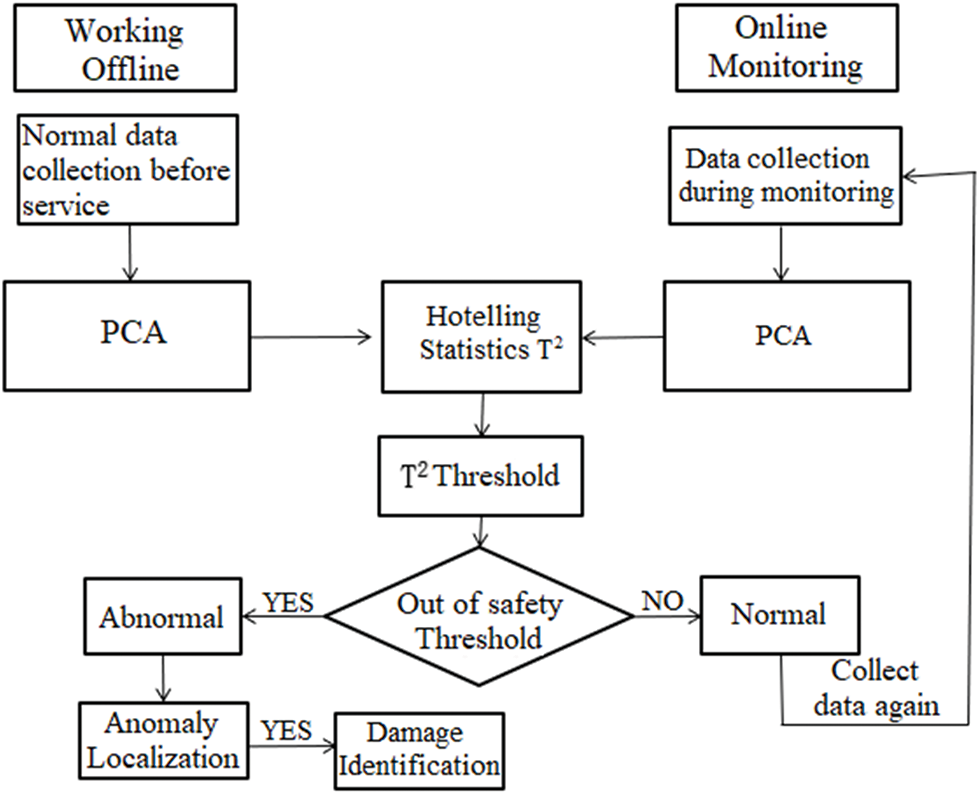
Figure 1: The flow chart of the MSWPCA method for structural health monitoring
The asymmetric double cantilever beam (ADCB) was used to investigate damage signals in honeycomb sandwich panel structures. To enhance the bonding strength between the sandwich and the aluminum alloy panel, both the upper and lower surfaces of the panels were polished with an angle grinder. A distributed optical fiber was embedded in the interface between the panel and the sandwich. A pre-fabricated debonding area measuring 75 mm × 60 mm was fabricated using a release cloth, as shown in Fig. 2. The panel and honeycomb sandwich structure were bonded using an epoxy resin adhesive film, which was hot pressed at 130°C for 3 h under a pressure of 0.3 MPa, as illustrated in Fig. 3.
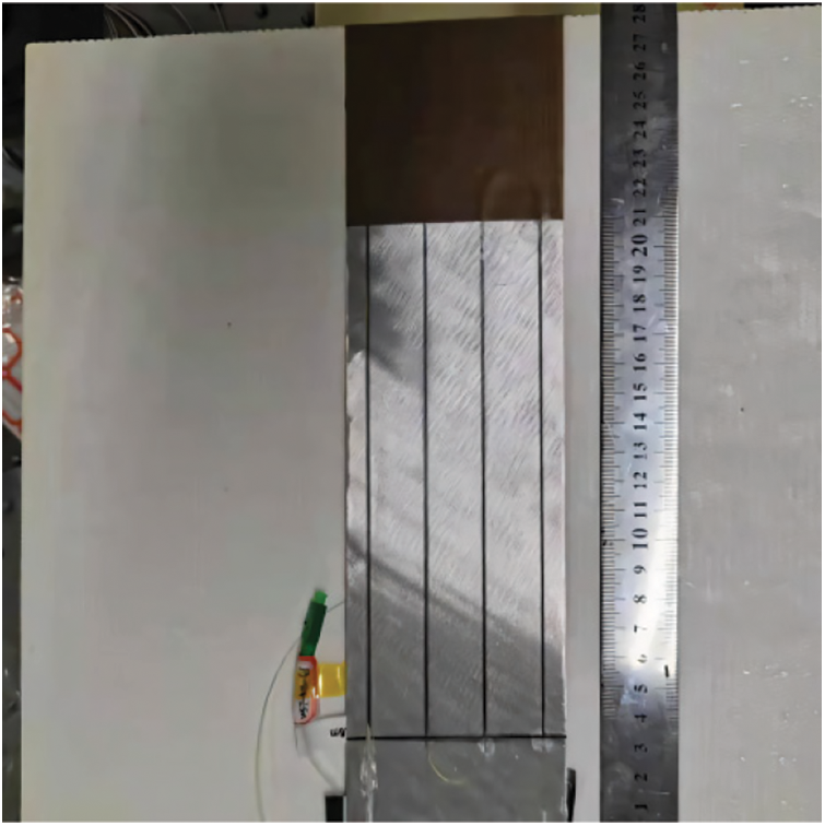
Figure 2: The optical fiber deployment path and prefabricated debonding area
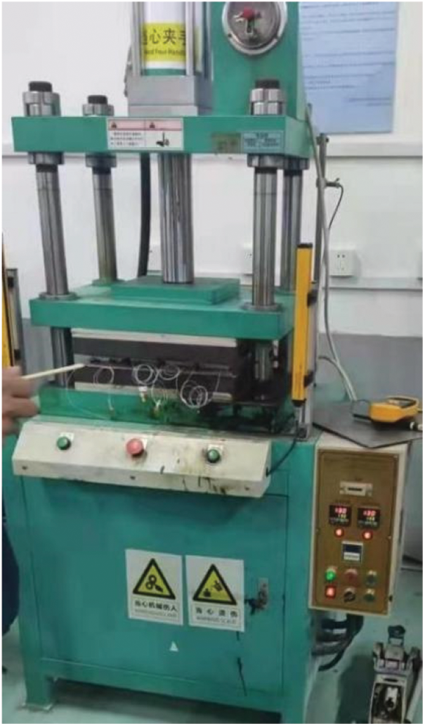
Figure 3: Hot pressing of specimens
The LUNA® ODiSI series demodulator, was used with the distributed optical fiber in this investigation, as shown in Fig. 4. ODiSI uses wavelength scanning interferometry to demodulate optical fiber sensors, which can detect physical changes in the sensor. The reflected light wavelength at a particular spot on the optical fiber will deviate if there is deformation there. It is feasible to determine which section has undergone deformation by contrasting the reflected light before and after deformation. By comparing such changes with a reference value, the current physical condition of the optical fiber can be inferred with precision. This physical phenomenon pertains to the interaction between temperature and strain manifested in optical fibers.
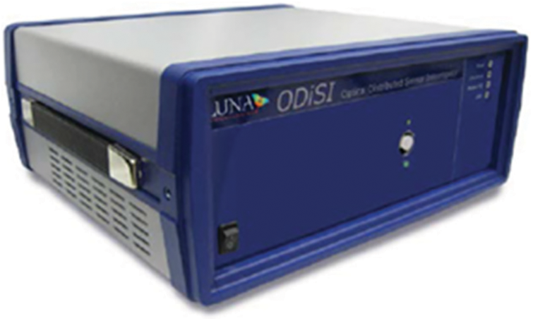
Figure 4: ODiSI A50 optical fiber sensing demodulator
The region of strain monitoring in an optical fiber partitioned into four distinct paths, and the initial coordinates of optical fiber points along the entire optical fiber within each monitoring area were pre-calibrated. The layout paths of the optical fiber and size specifications for the specimen model are depicted in Fig. 5.
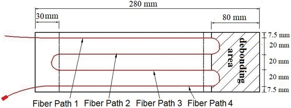
Figure 5: Optical fiber deployment path and specimen size
In accordance with the double cantilever beam tensile test standard, we made a fixture for the honeycomb sandwich panel structure. This fixture was then combined with the honeycomb sandwich panel specimen, as illustrated in Fig. 6. The upper and lower clamps were swiftly attached to the prefabricated debonding area at the honeycomb sandwich panel terminus using Elloda bonding. Additionally, a T-shaped clamp was affixed to the system with screws, enabling a seamless connection to a tensile testing machine for comprehensive tensile testing. Figs. 6 and 7 show the schematic and detailed drawings of the fixture.
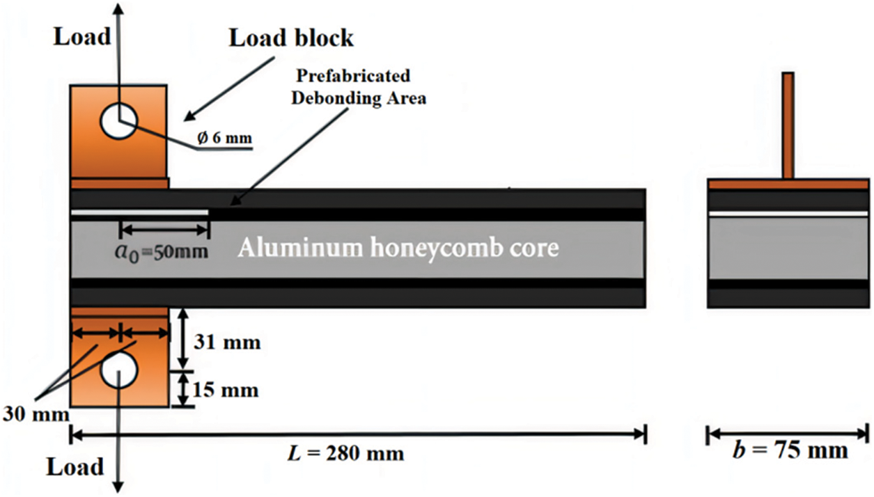
Figure 6: Schematic picture of ADCB experimental tensile fixture
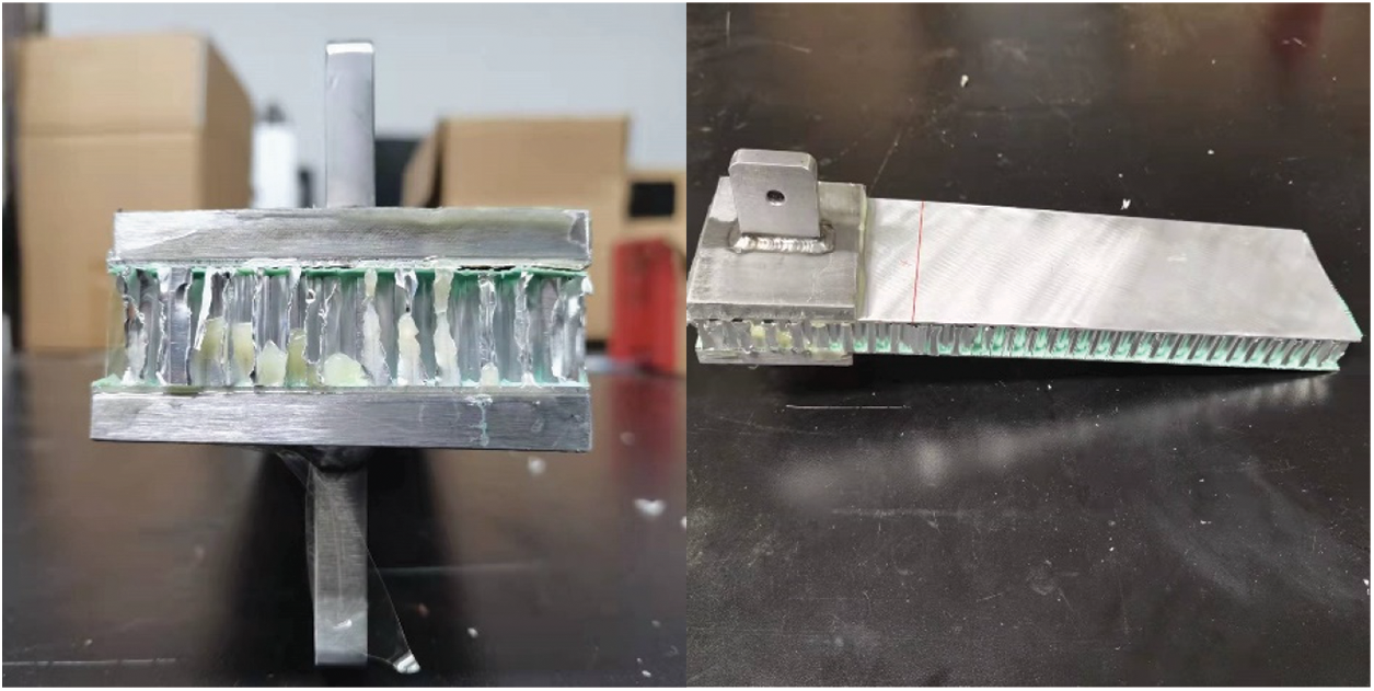
Figure 7: Physical picture of ADCB experimental tensile fixture
The experimental setup for the ADCB utilizes an Instron electronic universal tensile testing machine and quasi-static loading condition. The honeycomb sandwich test specimen was creating a seamless integration with the Instron tensile testing machine. The distributed optical fiber system was meticulously interfaced with the optical fiber demodulator through optical fiber jumpers, and a predefined set of benchmarks was established in advance.
The tensile testing machine was utilized to facilitate the loading process at a rate of 2 mm/min. Upon reaching a critical load of 0.3 KN, the prefabricated debonding area start to propagate along the panel-sandwich interface, as depicted in Fig. 8. The appearance of debonding propagation during successive loading cycles was presented in Fig. 9. The length of debonding extension was quantified by pausing the tensile test and marking the debonding front position by a marker, as illustrated in Fig. 10.
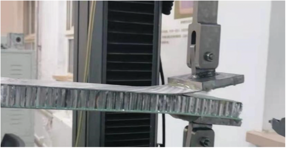
Figure 8: Opening of the prefabricated debonding area
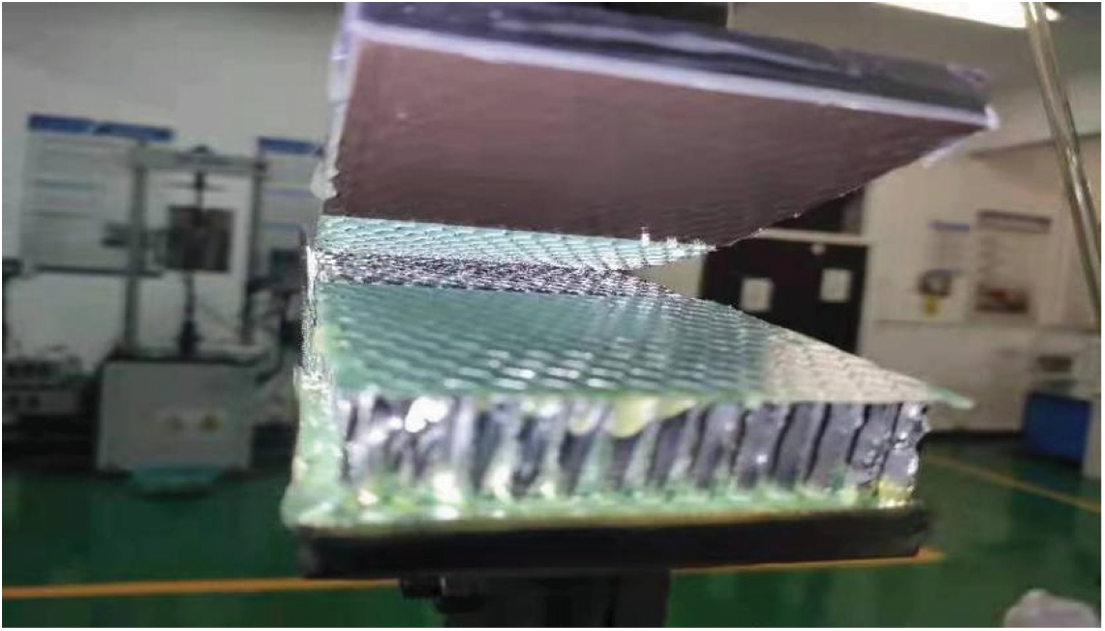
Figure 9: Debonding damage propagation
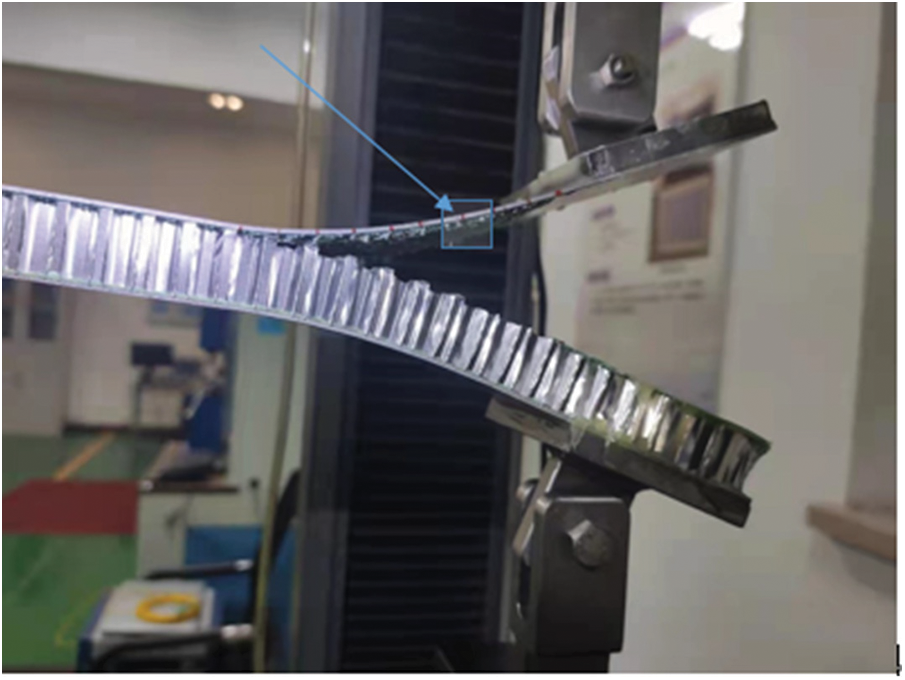
Figure 10: Mark the debonding propagation length
Simultaneously, strain data was obtained along the fiber path within the debonding region. The failure surface corresponded to a detachment between the honeycomb core and the upper aluminum plate surface. The optical fiber sensors were placed at the interface between the epoxy resin adhesive film and the aluminum alloy panel. This implies that the interface strength of the optical fiber sensor location surpassed that of the honeycomb core adhesive interface. Incorporating dispersed optical fiber sensors into the honeycomb sandwich panel structure exhibited negligible effects on the tensile attributes of the composite.
3.2 Optical Fiber Data Recording and PCA Result Analysis
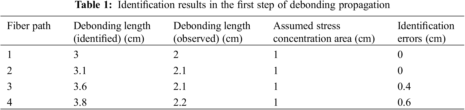
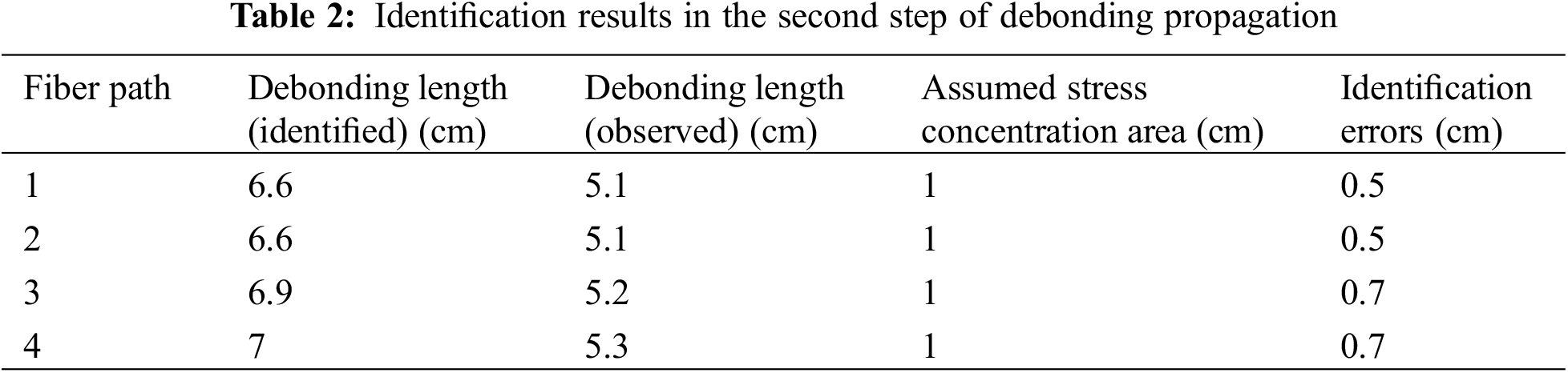
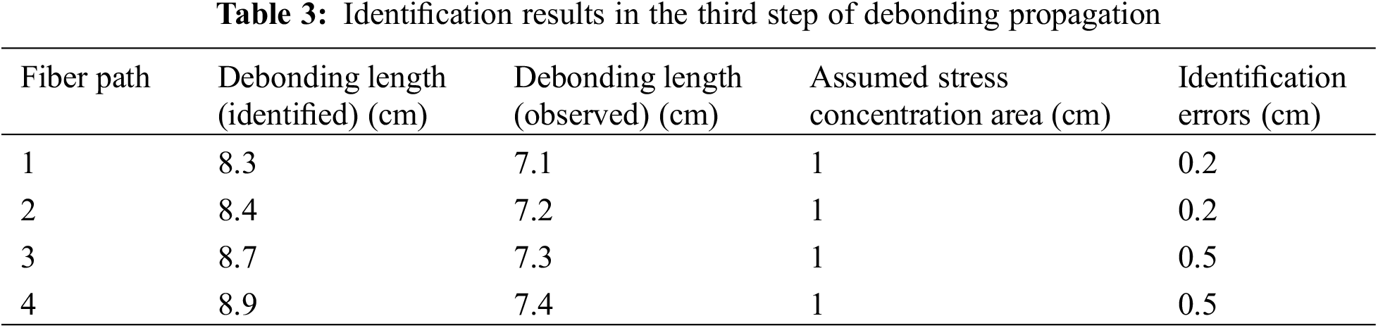
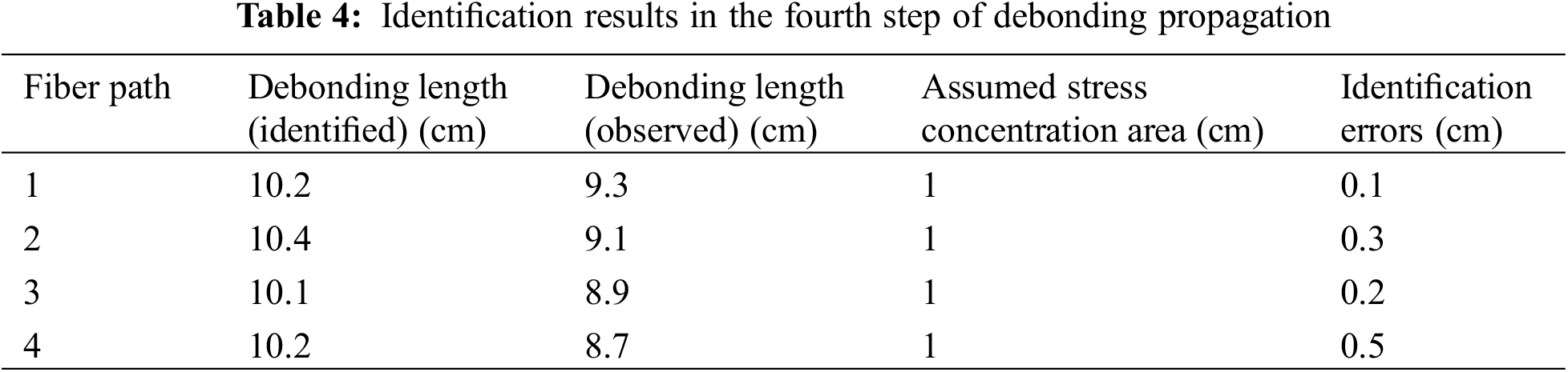
The zone at the front of the debonding exhibited a concentrated stress field, which spans approximately 1 cm in length [30,31]. As a result, the length of the debonding extension monitored during testing exceeds the actual debonding length by about 1 cm. Before conducting the loading test, 100 representative data sets were systematically collected and used as baseline data for PCA to establish a structural safety threshold. Although loading can cause some strain measurement errors, they were significantly smaller than the strain caused by structural damage. Therefore, the safety threshold should be moderately increased. To obtain abnormality regions, the test was intermittently paused to collect signal data during testing. Throughout the test, four distinct sets of experimental data were continuously monitored and entered into a PCA model.
The boundary information can be better distinguished by extending the data range and selecting 30 strain measurement points for the MSWPCA data area. We used a sliding window configuration to extract the data, with each set of data comprising 10 consecutive strain measurement points and a sliding window increment of 10 measurement points. Fig. 11 provides a visual illustration of this process.
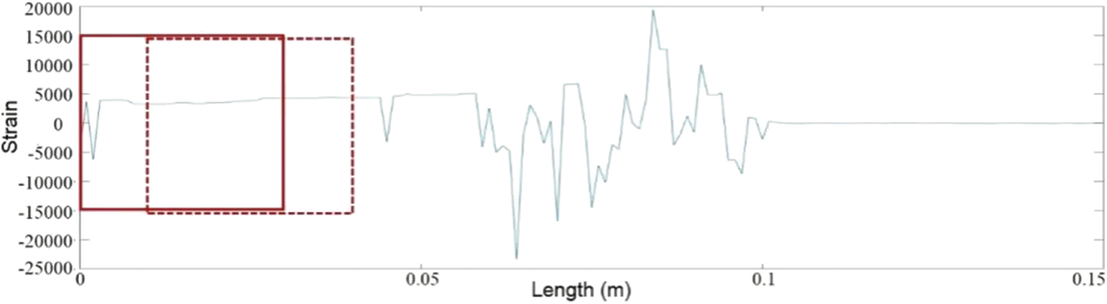
Figure 11: Optical fiber data for MSWPCA monitoring
Mathematically, the window size should be chosen to meet the statistical requirement of PCA to prevent too small sample size [32], and the sliding interval can be selected quite flexibly. However, the selection of window size and sliding interval should be in accordance with the actual need for damage identification (e.g., how small the debonding propagation can be detected). In particular, when dealing with discontinuous damage in the structure, an excessively large window may erroneously identify the intact area as damaged area.
Due to the continuous nature of the debonding region in the experimental setup, the corresponding abnormal signal appeared uniformly and continuously without any noticeable discontinuities. After performing PCA on each sub region by sliding window step, we monitored the debonding process starting from the first identified abnormal region and continued until a return to normalcy was detected within the given region. The debonding length along each fiber path can be presented by a formula, which roughly approximates the distance between the initial coordinates of the first anomalous window and those of the last window in a normal state. To determine the overall debonding length across the entire structure, we needed to compute an average value based on the debonding lengths obtained along four individual paths.
where Labnorm and Lnorm represent the first abnormal region and the last normal starting coordinates on each fiber path data, respectively. n = 4 represents four optical fiber paths. It should be noticed that the MSWPCA method is able to identify debondings in arbitrary directions if the optical fibers are deployed in those directions. In this study, however, the method was only used to identify debondings propagating along the length of the specimen and there were no optical fibers arranged in the perpendicular direction.
Since the honeycomb sandwich structure is heterogeneous and anisotropic, the debonding propagate irregularly and unevenly along the interface. Therefore, after the interfacial debonding propagate by around 7 mm (which is equal to the diameter of the honeycomb core), the specimen was unloaded at a rate of 2 mm per minute until the tensile load is zero. The strain information along the four fiber optic paths (as shown in Fig. 4) was collected, and the area of the debonding propagation was identified.
Each optical fiber measurement path consists of 150 strain measurement points, and 15 sets of characteristic strain data can be derived from each individual path. The data length coordinates were relative coordinates that were obtained from the calibration position of the optical fiber. The results of abnormality recognition using MSWPCA can be observed in Figs. 12–15, and are also presented in Tables 1–4. The total debonding length identified by the MSWPCA was indicated by the red box in the Figs. 12–15. In Tables 1–4, the debonding lengths identified according to the strain measurement signals and observed according to the red marks in Fig. 11 are presented. The length of the stress concentration area is assumed to be 1 cm, whereas the identification errors are calculated as the difference between the observed debonding length and the identified debonding length plus the length of the stress concentration area.
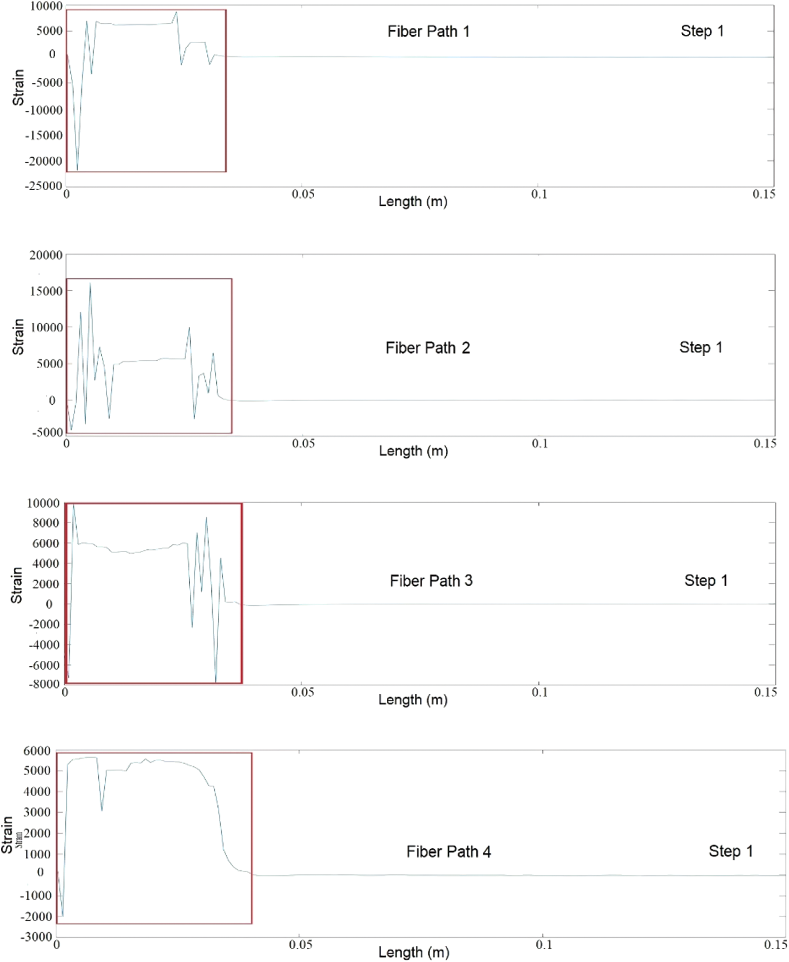
Figure 12: First debonding identification
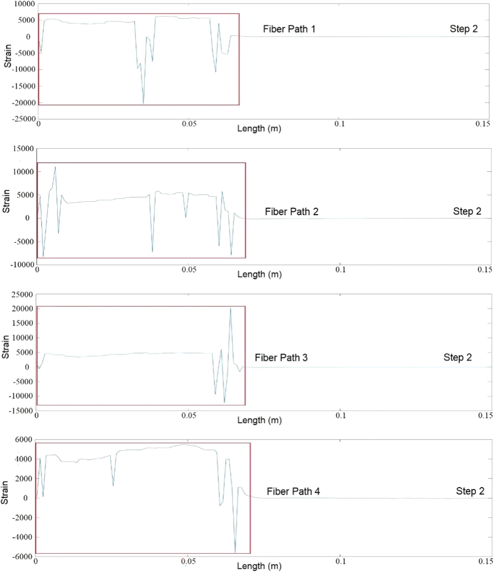
Figure 13: Second debonding identification
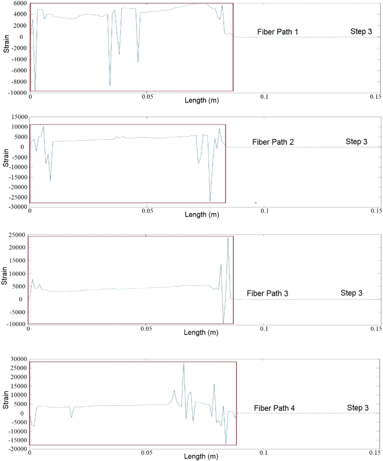
Figure 14: Third debonding identification
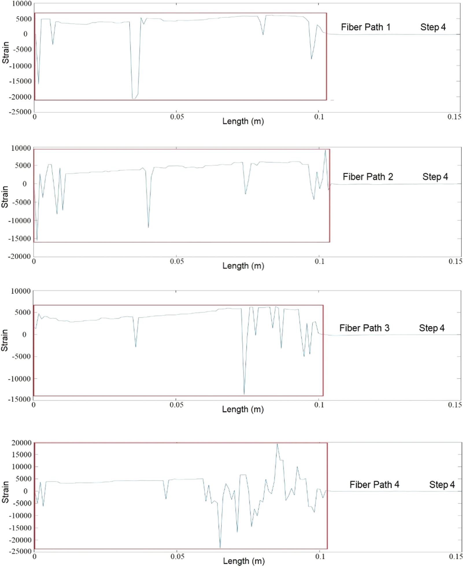
Figure 15: Debonding identification
Based on the previously discussed data analysis, it was evident that the debonding boundaries of distributed optical fibers undergo continuous changes throughout the loading test. Moreover, our findings indicate that the MSWPCA methodology demonstrates remarkable precision in accurately identifying the extension length of debonding within honeycomb face cores.
This paper presents a MSWPCA method in identify and tracking the propagation of debonding damage in honeycomb sandwich structures, relying on measurement signals from distributed fiber optic sensors.
(1) The MSWPCA can efficiently extract information from the static distributed strain signals measured on the structure, preventing the difficulties associated with manual evaluation of structural damage;
(2) Compared with other machine learning and deep learning methods such as ANN and CNN, PCA can be applied more conveniently without the need of massive data training, which is an important merit since the data amount from damaged structures is inherently limited;
(3) In contrast to conventional PCA techniques, the MSWPCA method makes use of data sliding window technology to not only recognize damage but also precisely quantify its propagation process.
The proposed method is also suitable for other kinds of strain sensors as long as the sensor’s measurement density is sufficient (e.g., quasi-distributed FBG sensors, Fabry-Perot fiber optic sensors, weak reflection fiber gratings). The developed approach offers technological assistance to the future development of online SHM systems.
Acknowledgement: None.
Funding Statement: This study is supported by the National Key Research and Development Program of China (No. 2018YFA0702800) and the National Natural Science Foundation of China (No. 12072056). The study is also supported by National Defense Fundamental Scientific Research Project (XXXX2018204BXXX).
Author Contributions: The authors confirm contribution to the paper as follows: study conception and design: Shuai Chen, Jianle Li, Hao Xu; data collection: Shuai Chen, Jianle Li, Song Zhang; analysis and interpretation of results: Shuai Chen, Song Zhang; draft manuscript preparation: Shuai Chen, Hao Xu; supervision: Zhanjun Wu; review and editing: Yinwei Ma, Zhongshu Wang. All authors reviewed the results and approved the final version of the manuscript.
Availability of Data and Materials: To access the data used in the study, it is possible to contact the corresponding author.
Conflicts of Interest: The authors declare that they have no conflicts of interest to report regarding the present study.
References
1. Rahul, V., Alokita, S., Jayakrishna, K., Kar, V. R., Rajesh, M. et al. (2019). Structural health monitoring of aerospace composites. In: Structural health monitoring of biocomposites, fibre-reinforced composites and hybrid composites, pp. 33–52. Cambridge: Woodhead Publishing. https://doi.org/10.1016/B978-0-08-102291-7.00003-4 [Google Scholar] [CrossRef]
2. Chen, R. F., Zuo, D. W., Sun, Y. L., Li, D. S., Lu, W. Z. et al. (2008). Investigation on strain films in the thin film resistance strain gauge. In: Key engineering materials, vol. 375, pp. 690–694. Stafa-Zurich, Switzerland: Trans Tech Publications, Ltd. https://doi.org/10.4028/www.scientific.net/KEM.375-376.690 [Google Scholar] [CrossRef]
3. Chen, J., Liu, B., Zhang, H. (2011). Review of fiber Bragg grating sensor technology. Frontiers of Optoelectronics in China, 4(2), 204–212. https://doi.org/10.1007/s12200-011-0130-4 [Google Scholar] [CrossRef]
4. Shin, C. S., Chiang, C. C. (2006). Fatigue damage monitoring in polymeric composites using multiple fiber Bragg gratings. International Journal of Fatigue, 28(10), 1315–1321. https://doi.org/10.1016/j.ijfatigue.2006.02.032 [Google Scholar] [CrossRef]
5. Glisic, B., Inaudi, D. (2012). Development of method for in-service crack detection based on distributed fiber optic sensors. Structural Health Monitoring, 11(2), 161–171. https://doi.org/10.1177/1475921711414233 [Google Scholar] [CrossRef]
6. Lu, P., Lalam, N., Badar, M., Liu, B., Chorpening, B. T. et al. (2019). Distributed optical fiber sensing: Review and perspective. Applied Physics Reviews, 6(4), 041302. https://doi.org/10.1063/1.5113955 [Google Scholar] [CrossRef]
7. Wang, H. P., Ni, Y. Q., Dai, J. G., Yuan, M. D. (2019). Interfacial debonding detection of strengthened steel structures by using smart CFRP-FBG composites. Smart Materials and Structures, 28(11), 115001. https://doi.org/10.1088/1361-665X/ab3add [Google Scholar] [CrossRef]
8. Leung, C. K., Wang, X., Olson, N. (2000). Debonding and calibration shift of optical fiber sensors in concrete. Journal of Engineering Mechanics, 126(3), 300–307. https://doi.org/10.1061/(ASCE)0733-9399(2000)126:3(300) [Google Scholar] [CrossRef]
9. García, I., Zubia, J., Durana, G., Aldabaldetreku, G., Illarramendi, M. A. et al. (2015). Optical fiber sensors for aircraft structural health monitoring. Sensors, 15(7), 15494–15519. https://doi.org/10.3390/s150715494 [Google Scholar] [PubMed] [CrossRef]
10. Cantero-Chinchilla, S., Chiachío, J., Chiachío, M., Chronopoulos, D., Jones, A. (2019). A robust Bayesian methodology for damage localization in plate-like structures using ultrasonic guided-waves. Mechanical Systems and Signal Processing, 122(3–5), 192–205. https://doi.org/10.1016/j.ymssp.2018.12.021 [Google Scholar] [CrossRef]
11. Vakil-Baghmisheh, M. T., Peimani, M., Sadeghi, M. H., Ettefagh, M. M. (2008). Crack detection in beam-like structures using genetic algorithms. Applied Soft Computing, 8(2), 1150–1160. https://doi.org/10.1016/j.asoc.2007.10.003 [Google Scholar] [CrossRef]
12. Mehrjoo, M., Khaji, N., Moharrami, H., Bahreininejad, A. (2008). Damage detection of truss bridge joints using artificial neural networks. Expert Systems with Applications, 35(3), 1122–1131. https://doi.org/10.1016/j.eswa.2007.08.008 [Google Scholar] [CrossRef]
13. Geng, P., Lu, J., Ma, H., Yang, G. (2023). Crack segmentation based on fusing multi-scale wavelet and spatial-channel attention. Structural Durability & Health Monitoring, 17(1), 1–22. https://doi.org/10.32604/sdhm.2023.018632 [Google Scholar] [CrossRef]
14. Kalyani, S., Rao, K. V., Sowjanya, A. M. (2021). A TimeImageNet sequence learning for remaining useful life estimation of turbofan engine in aircraft systems. Structural Durability & Health Monitoring, 15(4), 317–334. https://doi.org/10.32604/sdhm.2021.016975 [Google Scholar] [CrossRef]
15. Abdeljaber, O., Avci, O., Kiranyaz, M. S., Boashash, B., Sodano, H. et al. (2018). 1-D CNNs for structural damage detection: Verification on a structural health monitoring benchmark data. Neurocomputing, 275, 1308–1317. https://doi.org/10.1016/j.neucom.2017.09.069 [Google Scholar] [CrossRef]
16. An, Y. K., Jang, K., Kim, B., Cho, S. (2018). Deep learning-based concrete crack detection using hybrid images. Proceedings of Sensors and Smart Structures Technologies for Civil, Mechanical, and Aerospace Systems 2018, vol. 10598, pp. 273–284. Denver, Colorado, USA, SPIE. https://doi.org/10.1117/12.2294959 [Google Scholar] [CrossRef]
17. LeCun, Y., Bengio, Y., Hinton, G. (2015). Deep learning. Nature, 521(7553), 436–444. [Google Scholar] [PubMed]
18. Bao, Y., Li, H. (2021). Machine learning paradigm for structural health monitoring. Structural Health Monitoring, 20(4), 1353–1372. https://doi.org/10.1177/1475921720972416 [Google Scholar] [CrossRef]
19. Yi, T. H., Huang, H. B., Li, H. N. (2017). Development of sensor validation methodologies for structural health monitoring: A comprehensive review. Measurement, 109(5), 200–214. https://doi.org/10.1016/j.measurement.2017.05.064 [Google Scholar] [CrossRef]
20. Momeni, H., Ebrahimkhanlou, A. (2022). High-dimensional data analytics in structural health monitoring and non-destructive evaluation: A review paper. Smart Materials and Structures, 31(4), 043001. https://doi.org/10.1088/1361-665X/ac50f4 [Google Scholar] [CrossRef]
21. Rama, A., Kumar, S. K., Lakshmi, K. (2012). Sensor fault detection in large sensor networks using PCA with a multi-level search algorithm. Structural Durability & Health Monitoring, 8(3), 271–294. https://doi.org/10.32604/sdhm.2012.008.271 [Google Scholar] [CrossRef]
22. Pedro, F. (2010). A new method for maintenance management employing principal component analysis. Structural Durability & Health Monitoring, 6(2), 89–100. [Google Scholar]
23. Kruger, U., Dimitriadis, G. (2008). Diagnosis of process faults in chemical systems using a local partial least squares approach. AIChE Journal, 54(10), 2581–2596. https://doi.org/10.1002/aic.11576 [Google Scholar] [CrossRef]
24. Zhao, C., Wang, F., Jia, M. (2007). Dissimilarity analysis based batch process monitoring using moving windows. AIChE Journal, 53(5), 1267–1277. [Google Scholar]
25. Huang, H. B., Yi, T. H., Li, H. N. (2017). Bayesian combination of weighted principal-component analysis for diagnosing sensor faults in structural monitoring systems. Journal of Engineering Mechanics, 143(9), 4017088. [Google Scholar]
26. Joe Qin, S. (2003). Statistical process monitoring: Basics and beyond. Journal of Chemometrics, 17(8–9), 480–502. [Google Scholar]
27. Bonetto, P., Qi, J., Leahy, R. M. (2000). Covariance approximation for fast and accurate computation of channelized Hotelling observer statistics. IEEE Transactions on Nuclear Science, 47(4), 1567–1572. [Google Scholar]
28. Aparisi, F. (1996). Hotelling’s T2 control chart with adaptive sample sizes. International Journal of Production Research, 34(10), 2853–2862. [Google Scholar]
29. Lima, F. C. E., Almeida, C. A. S. (2021). Phase transitions in the logarithmic Maxwell O(3)-sigma model. The European Physical Journal C, 81, 1044. https://doi.org/10.1140/epjc/s10052-021-09826-x [Google Scholar] [CrossRef]
30. Beyerlein, I. J., Phoenix, S. L. (1996). Stress concentrations around multiple fiber breaks in an elastic matrix with local yielding or debonding using quadratic influence superposition. Journal of the Mechanics and Physics of Solids, 44(12), 1997–2039. https://doi.org/10.1016/S0022-5096(96)00068-3 [Google Scholar] [CrossRef]
31. van den Heuvel, P. W. J., Peijs, T., Young, R. J. (1998). Failure phenomena in two-dimensional multi-fibre microcomposites—3. A raman spectroscopy study of the influence of interfacial debonding on stress concentrations. Composites Science and Technology, 58(6), 933–944. https://doi.org/10.1016/S0266-3538(97)00216-9 [Google Scholar] [CrossRef]
32. Lakens, D. (2022). Sample size justification. Collabra: Psychology, 8(1), 33267. https://doi.org/10.1525/collabra.33267 [Google Scholar] [CrossRef]
Cite This Article
 Copyright © 2024 The Author(s). Published by Tech Science Press.
This work is licensed under a Creative Commons Attribution 4.0 International License , which permits unrestricted use, distribution, and reproduction in any medium, provided the original work is properly cited.
 Downloads
 Citation Tools