LaNets: Hybrid Lagrange Neural Networks for Solving Partial Differential Equations

1  Introduction

In this paper, we consider partial differential equations (PDEs) of the general form in Eqs. (1.1)–(1.3):

ut+Lu(t,x)=f,t∈[0,T],x∈Ω,(1.1)

u(0,x)=u0,x∈Ω,(1.2)

u(t,x)=uΓ,t∈[0,T],x∈∂Ω,(1.3)

where L is a differential operator, Ω is a subset of RN, and ∂Ω represents its boundary. u denotes the unknown function that needs to be solved, u0 and uΓ represent initial and boundary conditions, respectively. Different governing equations and homologous initial/boundary conditions can describe many physical phenomena in nature, but it is practically difficult to find the analytical solutions. Therefore, more and more scholars have tried a variety of numerical methods to solve PDEs in recent years.

At first, traditional numerical methods, including finite element method [1], finite volume method [2] and finite difference method [3], were usually used to solve partial differential equations. Afterwards, with the rapid development of machine learning [4–6], the universal approximation ability of neural networks is considered to be helpful for obtaining approximated solutions of differential equations. Han et al. [7–9] proposed deep learning-based numerical approaches to solve variational problems, backward stochastic differential equations and high-dimensional equations. Then Chen et al. [10] extended their work to solve Navier-Stokes and Cahn-Hillard equation. Sirignano et al. [11] combined Galerkin method and deep learning to solve high-dimensional free boundary PDEs. Raissi et al. [12] proposed the physics-informed neural network (PINNs) framework which acts as the benchmark algorithm in this field. In PINNs, physical constraints are added to limit the space of solutions to improve the accuracy. Futhermore, many scholars carry out research based on this method. Dwivedi et al. [13] incorporated PINNs with extreme learning machine to solve time-dependent linear partial differential equations. Pang et al. [14] solved space-time fractional advection-diffusion equations by expanding PINNs to fractional PINNs. Raissi et al. [15] subsequently developed a physics-informed deep learning framework that is able to encode Navier-Stokes equations into the neural networks. Kharazmi et al. [16] constructed a variational physics-informed neural network to effectively reduce the training cost in network training. Yang et al. [17] proposed Bayesian physics-informed neural networks for solving forward and inverse nonlinear problems with PDEs and noisy data. Meng et al. [18] developed a parareal physics-informed neural network to significantly accelerate the long-time integration of partial differential equations. Gao et al. [19] proposed a new learning architecture of physics-constrained convolutional neural network to learn the solutions to parametric PDEs on irregular domains.

Neural network is a black box model, its approximation ability depends partly on the depth and width of the network, and thus too many parameters will cause a decrease in computational efficiency. One may use Functional Link Artificial Neural Network (FLANN) [20] model to overcome this problem. In FLANN, the single hidden layer of neural network is replaced by an expansion layer based on distinct polynomials. Mall et al. [21] used Chebyshev neural network to solve elliptic partial differential equations by replacing the single hidden layer of the neural network with Chebyshev polynomials. Sun et al. [22] replaced the hidden layer with Bernstein polynomials to obtain the numerical solution of PDEs as well. Due to the application of polynomials, neural network has no actual hidden layers, and the number of parameters is greatly reduced.

On the other hand, deep learning is a type of learning that requires a lot of data. The performance of deep learning depends on large-scale and high-quality sample sets but the cost of data acquisition is prohibitive. Moreover, sample labeling also needs to consume a lot of human and material resources. Therefore, a popular learning paradigm named Small Sample Learning (SSL) [23] has been used in some new fields. SSL refers to the ability to learn and generalize under a small number of samples. At present, SSL has been successfully applied in medical image analysis [24], long tail distribution target detection [25], remote sensing scene classification [26], etc.

In this paper, we integrate Lagrange interpolation and small sample learning with deep neural networks frameworks to deal with the problems in existing models. Specifically, we replace the first hidden layer of the deep neural network with a Lagrange block. Here, Lagrange block is a pre-processing tool for preliminary fitting and feature extraction of input data. The Lagrange basis function has a neat structure and strong expressive ability, so it is fully capable of better extracting detailed features of input data for feature enhancement. The main thought of Lagrange interpolation is to interpolate the function values of other positions between nodes through the given nodes, so as to make a prefitting behaviour without adding any extra parameters. Then, the enhanced vector is input to the subsequent hidden layer for the training of the network model. Furthermore, we add the residual of a handful of observations into cost function to rectify the model and improve the predictive accuracy with less label data. This composite neural network structure is quite flexible, mainly in that the structure is easy to modify. That is, the number of polynomials and hidden layers can be adjusted according to the complexity of different problems.

The structure of this paper is as follows. In Section 2, we present the introduction of Lagrange polynomials, the structure of the LaNets and the steps of algorithm. Numerical experiments for one-dimensional PDEs and two-dimensional PDEs are described in Section 3. Finally, conclusions are incorporated into Section 4.

2  LaNets: Theory, Architecture, Algorithm

In this section, we start with illustrations on Lagrange interplotation polymonials. After that, we discuss the framework of LaNets. And finally, we clarify the detatils of the proposed algorithm.

2.1 Lagrange Interpolation Polynomial

Lagrange interpolation is a kind of polynomial interpolation methods proposed by Joseph-Louis Lagrange, a French mathematician in the 18th century, for numerical analysis [27]. Interpolation is an important method for the approximation of functions, which uses the value of a function at a finite point to estimate the approximation of the function at other points. That is, the continuous function is interpolated on the basis of discrete data to make the continuous curve pass through all the given discrete data points. Mathematically speaking, Lagrange interpolation can give a polynomial function that passes through several known points on a two-dimensional plane.

Assuming x1,x2,…,xn+1 are the distinct n+1 points in the complex panels, and y1,y2,…,yn+1 are the corresponding values at x1,x2,…,xn+1. The Lagrange polynomial L(x) corresponding to their degree not exceeding n is unique. Indeed, the uniqueness of L(x) arises from the fact that the difference of two such polynomials vanish at points x1,…,xn+1 without a degree greater than n. The following polynomial clearly possesses all the necessary properties in Eqs. (2)–(3):

L(x)=∑j=1n+1yj(x−x1)⋅⋅⋅(x−xj−1)⋅(x−xj+1)⋅⋅⋅(x−xn+1)(xj−x1)⋅⋅⋅(xj−xj−1)⋅(xj−xj+1)⋅⋅⋅(xj−xn+1)=∑j=1n+1yjw(x)(x−xj)w′(xj),(2)

where

w(x)=(x−x1)⋅⋅⋅(x−xn+1).(3)

Here, the polynomial L(x) is called Lagrange interpolation polynomial. And the distinct points x1,…,xn+1 are called the interpolation points. It can be seen that the corresponding Lagrange polynomial can be obtained by given n+1 value points: (x0,y0),…,(xn,yn). The Lagrange interpolation polynomial obtained from only some points can replace the function to obtain the solution at any other points. The correctness of Lagrange polynomials has been proved in the literatures [27,28].

2.2 The Architecture of LaNets

Fig. 1 displays the structure of LaNets, which is composed of two main parts. One is a preprocessing part based on Lagrange polynomials, the other is the training of deep feedforward neural network. Thus, the LaNets model we designed is a joint feedforward neural network composed of input layer, Lagrange block, hidden layers and output layer. As described in Section 2.1, we can also write Lagrange interpolation polynomial in Eq. (4):

L(x):=∑j=0kyjlj(xj),(4)

where xj and yj in the above formula correspond to the position of the independent variable and the value of function at this position, respectively. Here, we call lj(x) the Lagrange interpolation basis function, and the expression of lj(x) is as follows:

lj(x):=∏i=0,i≠jkx−xixj−xi=x−x0xj−x0⋅⋅⋅x−xj−1xj−xj−1⋅x−xj+1xj−xj+1⋅⋅⋅x−xkxj−xk.(5)

Figure 1: The schematic drawing of the LaNets

As shown in Fig. 1, the original input vector is extended to a new enhanced vector by Lagrange block primarily, and then sent to deep feedforward neural network for training. The black Lagrange block on the right shows the Lagrange interpolation basis functions l0, l1 and l2 visually. Spatio-temporal variables can be both handled with Lagrange basis functions. Actually, the proposed model not only increases the reliability and stability of the single-layer polynomial neural network, but also improves the predictive accuracy of the deep feedforward neural network without adding any extra parameters.

2.3 Loss Function & Algorithm

The problem we aim to solve is described as Eqs. (1.1)–(1.3). Following the original work of Raissi et al. [12], F(t,x) can be defined as Eq. (6):

F:=ut+Lu−f.(6)

We continue to approximate u(t,x) with the deep neural network u(t,x;θ), where θ represents the parameter set of the network. The model is then trained by minimizing the following compound loss function J(θ) in Eq. (7):

J(θ)=1Nu∑i=1Nu(u(tui,xui)−ui)2+1Nin∑i=1Nin(u(tini,xini)−ui)2+1Nf∑i=1Nff(tfi,xfi)2.(7)

Here, (tui,xui,ui)i=1Nu denotes the initial and boundary value, (tini,xini,ui)i=1Nin represents the small sample data on u(t,x), and (tfi,xfi)i=1Nf specifies the collocation points on f(t,x). The first loss term satisfies the initial and boundary conditions, the second term corresponds to the residuals of the small sample data on the domain and the third term serves as a constraint on the governing equation itself. The optimization method used here is L-BFGS-B algorithm [29], which converges faster in calculations and has lower memory overhead.

An entire overview of this work is shown in Algorithm 1. In the algorithm description, we consider the spatio-temporal variables x and t. Without a doubt, the proposed method is also applicable to time-independent partial differential equations, and related examples will be mentioned in the following experiments.

3  Numerical Experiments

In this section, we verify the performance and accuracy of LaNets numerically through experiments with benchmark equations. In Subsection 3.1, we provide three typical one-dimensional time-dependent PDEs to validate the robustness and validity of the proposed algorithm. In Subsection 3.2, two-dimensional PDEs are shown to illustrate the reliability and stability of the method.

3.1 Numerical Results for One-Dimensional Equations

In this subsection, we demonstrate the predictive accuracy of our method on three one-dimensional time-dependent PDEs including Burgers equation, carburizing constant diffusion coefficient equation and carburizing variable diffusion coefficient equation.

3.1.1 Burgers Equation

We start with the following one-dimensional time-dependent Burgers equation in Eqs. (8.1)–(8.3):

ut+u⋅ux=λ⋅uxx,x∈[−1,1],t∈[0,1],(8.1)

u(0,x)=−sin(π⋅x),(8.2)

u(t,−1)=u(t,1)=0,(8.3)

where λ is the viscosity parameter. In this case, we take λ=0.01/π.

Here, the LaNets model consists of one Lagrange block and 7 hidden layers with 20 neurons in each layer. Lagrange block contains three Lagrange basis functions. By default, the Lagrange block is composed of three Lagrange basis functions unless otherwise specified. Fig. 2a illustrates the predicted numerical result of the Burgers equation, and the relative L2 error measured at the end is 3.84×10−4. The loss curve vs. iteration is displayed in Fig. 2b. The mean square error loss decreases steadily, which illustrates the stability of the proposed method.

Figure 2: (a) The predicted solution of one-dimensional Burgers equation. Here, we adopt a 9-layer LaNets. The size of small sample points is 100. The relative L2 error measured is 3.84×10−4. (b) The loss curve vs. iteration

To further verify the effectiveness of the proposed algorithm, we compare the predicted solution with the analytical solution provided in the literature [30] at four timesnapshots, which are presented in Fig. 3. It seems that there is almost no difference between the predicted solution and the exact solution. Moreover, the sharp gap formed near time t=0.65 is also well captured.

Figure 3: The comparison of predicted solutions obtained by LaNets and exact solutions at four time snapshots t=(0.1,0.25,0.65,0.99) for the one-dimensional Burgers equation

A more detailed numerical result is summarized in Table 1. It has to be noted that the early work [31] serves as a benchmark. In order to observe the influence of a different number of small sample points in the algorithm, we add 50 small sample points each time to calculate the corresponding results. From Table 1, one can visually see that the error of the LaNets model is one order of magnitude lower than that of PINNs. In addition, we can clearly find that 50 sample points used here can achieve a higher predictive accuracy than the 300 sample points used in the benchmark model. It means that using less label data to get more accurate predicted results is achievable, thereby saving a lot of manpower and material resources and increasing computational efficiency.

3.1.2 Carburizing Diffusion Model

We consider the one-dimensional carburizing diffusion model [32] in Eqs. (9.1)–(9.4):

ut=(D(u)⋅ux)x,x∈[l,r],t∈[0,T],(9.1)

u(0,x)=u0(x),x∈[l,r],(9.2)

u(t,l)=ul,t∈[0,T],(9.3)

u(t,r)=ur,t∈[0,T],(9.4)

where D(u) represents the diffusion coefficient and u is the concentration of carbon. Here, l and r denote the left and right boundary of the model. Diffusion is a fundamental process of carburizing, and the diffusion coefficient is related to temperature, the content of alloy elements, systems, etc. Next we consider carburizing diffusion equation with constant and variable diffusion coefficient, respectively.

1.    Constant diffusion coefficient

We start with the constant diffusion coefficient D(u) according to Eq. (10):

D(u)=D0⋅exp(−Q/(RT2)),(10)

where D0, Q, R and T2 are already given. In a practical sense, D0 represents the pre-exponential factor, Q denotes the activation energy of carbon, R describes the gas constant and T2 is the temperature during the carburizing process (K).

In this numerical experiment, we take D0=16.2mm2/s, Q=137800J/mol, R=8.314J/(K×mol) and T2=1123K. The corresponding exact solution is written as Eq. (11):

u(t,x)=up−(up−ud)erf(x/(2⋅D⋅t)),(11)

where we have up=1.2 and ud=0.2. The terminal time T of this model is 36000, the left boundary l is 0, and the right boundary r is 2.5.

Regarding the training set, we take Nu=150,Nin=300,Nf=10000. Moreover, we employ a 8-layer LaNets to represent the solution u(t,x) in this simulation. The LaNets model contains one Lagrange block, six hidden layers with 20 hidden neurons per layer and one output layer. Here, the relative L2 error is measured at 1.35×10−3.

In order to evaluate the performance of our algorithm in multiple ways, we compare the simulation results with the simulation results obtained by the PINNs model and our earlier model. The results for the three models are shown in Fig. 4. We can clearly see that the predicted solution of the PINNs model is not quite consistent with the exact solution, and the differences become more and more obvious over time. And it is here that the LaNets model fits more accurately than the benchmark model. Thus, the proposed method has obvious advantages in the long time simulation of time-dependent partial differential equations. A more intuitive error value obtained by three algorithms is listed in Table 2, from which we find that the predicted error of the benchmark model is one order of magnitude lower than PINNs. Meanwhile, the predicted error of LaNets when using 300 sample points is almost one order of magnitude lower than the benchmark model. The decline curve of the loss function in the training process is shown in the Fig. 5a. It can be seen that the loss has been declined to a small value in few iterations during the training process.

Figure 4: Predicted solutions for one-dimensional carburizing constant diffusion coefficient equation. Top row: LaNets model; Middle row: benchmark model; bottom row: PINNs model. First column: t=0.1h; Middle column: t=1.0h; last column: t=10.0h

Figure 5: (a) The loss curve vs. iteration for the one-dimensional carburizing diffusion equation with constant diffusion coefficient. (b) The loss curve vs. iteration for the one-dimensional carburizing diffusion equation with variable diffusion coefficient

2.   Variable diffusion coefficient

In this experiment, the carburizing diffusion coefficient D(u) varies with the temperature, systems and ratio of the element. Here, we consider D(u)=cosu, and add a source term s(t,x) as Eq. (12):

s(t,x)=sin(e−d⋅t⋅sinx)⋅e−2d⋅t⋅cos2x−d⋅e−d⋅t⋅sinx+cos(e−d⋅t⋅sinx)⋅e−d⋅t⋅sinx.(12)

The analytical solution corresponding to this setting is Eq. (13):

u(t,x)=sinx⋅e−d⋅t.(13)

In this example, we have d=0.5, the left boundary l=−π, the right boundary r=π and the ending time T=1. Moreover, we use a 8-layer LaNets to denote the spatio-temporal solution u(t,x). The curve of loss function during training is shown in the Fig. 5b.

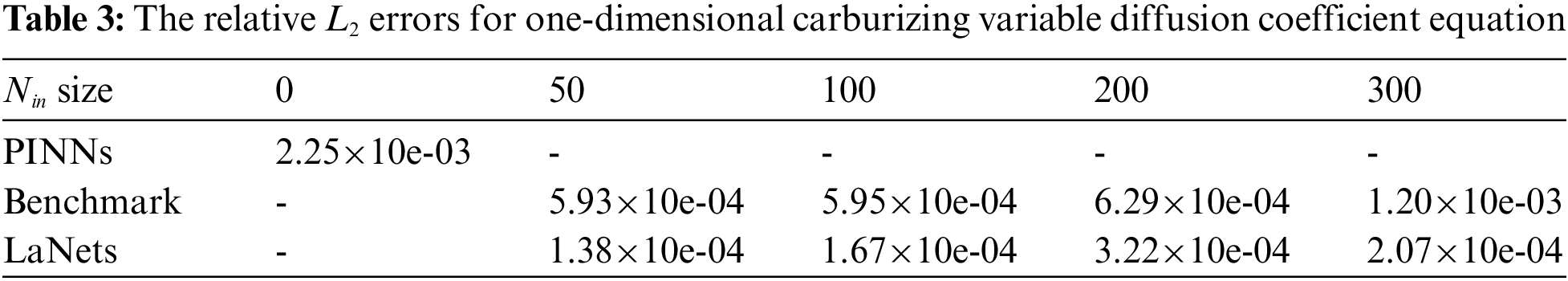
Further, we make a contrast between the simulation results obtained by the proposed model and the benchmark model. The detailed results for them are displayed in Fig. 6. While all experimental results seem to be consistent with the analytical results, one can find that the predicted solution of the LaNets model is more closer to the exact solution. A more accurate error evaluation is summarized in Table 3, from which we see that the prediction error of the LaNets model is always lower than that of the benchmark model when using the same number of small sample points.

Figure 6: Predicted solutions for one-dimensional carburizing variable diffusion coefficient equation. Top row: LaNets model; bottom row: benchmark model. First column: t=0.1; middle column: t=0.5; last column: t=1.0

3.2 Numerical Results for Two-Dimensional Equations

In this section, we consider two-dimensional problems including the time-independent Helmholtz equation and time-dependent Burgers equation to verify the effectiveness of the LaNets model. These two types of two-dimensional problems aim to demonstrate the generalization ability of our methods.

3.2.1 Helmholtz Equation

In this example, we consider a time-independent two-dimensional Helmholtz equation as Eq. (14):

uxx+uyy+k2(u)−f(x,y)=0.(14)

with homogeneous Dirichlet boundary conditions and the source function f(x,y) is given by Eq. (15):

f(x,y)=2⋅π⋅cos(π⋅x)⋅sin(π⋅y)+2⋅πcos(π⋅y)⋅sin(π⋅x)+(x+y)⋅sin(π⋅x)sin(π⋅y)−2⋅π2⋅(x+y)⋅sin(π⋅x)⋅sin(π⋅y),[x,y]∈[−1,1]2.(15)

Here, we take k=1 and the analytical solution is Eq. (16):

u(x,y)=(x+y)⋅sin(π⋅x)⋅sin(π⋅y).(16)

The training set of this example is generated according to the exact solution in the above equation. The problem is solved using the 4-layer LaNets model on the domain [−1,1]×[−1,1]. And each hidden layer consists of 40 hidden neurons. The relative L2 error measured is 5.28×10−4. The training set is specified as Nu=400,Nin=200,Nf=10000.

The visual comparison among LaNets, benchmark and PINNs results is displayed in Fig. 7. From Fig. 7, we find that the predicted solution of the benchmark model is not quite consistent with the exact solution. In addition, the proposed model is more accurate than the PINNs model especially on the boundary. Detailed error values for the three models are shown in Table 4, from which we see that the predicted error of the LaNets model is always minimal. The loss curve during the training process is shown in Fig. 8a. From Fig. 8a, we see that the value of the loss decreases continuously and smoothly from a higher value to a lower value, which shows the stability and robustness of the proposed model.

Figure 7: Predicted solutions for the two-dimensional Helmholtz equation. Top row: LaNets model; Middle row: benchmark model; bottom row: PINNs model. First column: x=−0.8; middle column: x=0.1; last column: x=0.5

Figure 8: (a) The loss curve vs. iteration for two-dimensional Helmholtz equation. (b) The loss curve vs. iteration for two-dimensional Burgers equation

3.2.2 2D Burgers Equation

In the last experiment, we consider a two-dimensional time-dependent Burgers equation as Eq. (17):

ut+u⋅(ux+uy)−λ⋅(uxx+uyy)=0,(x,y)∈[0,1]×[0,1],t∈[0,T],(17)

where u represents the predicted spatio-temporal solution. The corresponding initial and boundary conditions are given by Eq. (18):

u(t,x,y)=11+exp(x+y−t2⋅λ))(18)

In this example, we take λ=0.1 and T=3. The training set is generated by the exact solution Eq. (18), which is utilized to assess the accuracy of our method. The computing domain is set to [0,1]×[0,1]×[0,3]. We apply an 8-layer LaNets model and each hidden layer consists of 20 neurons. The residual training points are 20000 and the initial and boundary points are 150 whereas the Nin points are 300.

The decline curve of the loss function is shown in Fig. 8b. It can be seen that the loss value drops steadily to a small value over fewer iterations. Fig. 9 displays the 3D plot of the solution at t=0.5, and the relative L2 error calculated is 2.06×10−4. The experiment of the two-dimensional time-dependent Burgers equation proves that the proposed method can effectively solve high-dimensional time-dependent PDEs. In theory, the LaNets model can solve PDEs in arbitrary dimensions, and the remaining research is left for future work. The detailed relative L2 errors obtained by LaNets, benchmark and PINNs are given in Table 5, from which we can know that the predicted error of LaNets is lower than that of the benchmark model and PINNs model.

Figure 9: The predicted solution of the two-dimensional Burgers equation at t=0.5

4  Conclusion

In this paper, we propose hybrid Lagrange neural networks called LaNets to solve partial differential equations. We first perform Lagrange interpolation through Lagrange block in front of deep feedforward neural network architecture to make pre-fitting and feature extraction. Then we add the residuals of small sample data points in the domain into the cost function to rectify the model. Compared with the single-layer polynomial network, LaNets greatly increase the reliability and stability. And compared with general deep feedforward neural network, the proposed model improves the predictive accuracy without adding any extra parameters. Moreover, the proposed model can obtain more accurate prediction with less label data, which makes it possible to save a lot of manpower and material resources and improve computational efficiency. A series of experiments demonstrate the effectiveness and robustness of the proposed method. In all cases, our model shows smaller predictive errors. The numerical results verify that the proposed method improves the predictive accuracy, robustness and generalization ability.

Acknowledgement: This research was supported by NSFC (No. 11971296), and National Key Research and Development Program of China (No. 2021YFA1003004).

Funding Statement: The authors received no specific funding for this study.

Conflicts of Interest: The authors declare that they have no conflicts of interest to report regarding the present study.

References

 1.  Taylor, C. A., Hughes, T. J., Zarins, C. K. (1998). Finite element modeling of blood flow in arteries. Computer Methods in Applied Mechanics and Engineering, 158(1–2), 155–196. DOI 10.1016/S0045-7825(98)80008-X. [Google Scholar] [CrossRef]

 2.  Eymard, R., Gallouët, T., Herbin, R. (2000). Finite volume methods. Handbook of Numerical Analysis, 7, 713–1018. DOI 10.4249/scholarpedia.9835. [Google Scholar] [CrossRef]

 3.  Zhang, Y. (2009). A finite difference method for fractional partial differential equation. Applied Mathematics and Computation, 215(2), 524–529. DOI 10.1016/j.amc.2009.05.018. [Google Scholar] [CrossRef]

 4.  Jordan, M. I., Mitchell, T. M. (2015). Machine learning: Trends, perspectives, and prospects. Science, 349(6245), 255–260. DOI 10.1126/science.aaa8415. [Google Scholar] [CrossRef]

 5.  Lake, B. M., Salakhutdinov, R., Tenenbaum, J. B. (2015). Human-level concept learning through probabilistic program induction. Science, 350(6266), 1332–1338. DOI 10.1126/science.aab3050. [Google Scholar] [CrossRef]

 6.  LeCun, Y., Bengio, Y., Hinton, G. (2015). Deep learning. Nature, 521(7553), 436–444. DOI 10.1038/nature14539. [Google Scholar] [CrossRef]

 7.  Han, J., Jentzen, A., Weinan, E. (2018). Solving high-dimensional partial differential equations using deep learning. Proceedings of the National Academy of Sciences, 115(34), 8505–8510. DOI 10.1073/pnas.1718942115. [Google Scholar] [CrossRef]

 8.  Weinan, E., Han, J., Jentzen, A. (2017). Deep learning-based numerical methods for high-dimensional parabolic partial differential equations and backward stochastic differential equations. Communications in Mathematics and Statistics, 5(4), 349–380. DOI 10.1007/s40304-017-0117-6. [Google Scholar] [CrossRef]

 9.  Han, J., Zhang, L., Weinan, E. (2019). Solving many-electron schrödinger equation using deep neural networks. Journal of Computational Physics, 399, 108929. DOI 10.1016/j.jcp.2019.108929. [Google Scholar] [CrossRef]

10. Chen, Y., He, Q., Mei, M., Shi, X. (2018). Asymptotic stability of solutions for 1-D compressible navier–Stokes–Cahn–Hilliard system. Journal of Mathematical Analysis and Applications, 467(1), 185–206. DOI 10.1016/j.jmaa.2018.06.075. [Google Scholar] [CrossRef]

11. Sirignano, J., Spiliopoulos, K. (2018). DGM: A deep learning algorithm for solving partial differential equations. Journal of Computational Physics, 375, 1339–1364. DOI 10.1016/j.jcp.2018.08.029. [Google Scholar] [CrossRef]

12. Raissi, M., Perdikaris, P., Karniadakis, G. E. (2019). Physics-informed neural networks: A deep learning framework for solving forward and inverse problems involving nonlinear partial differential equations. Journal of Computational Physics, 378, 686–707. DOI 10.1016/j.jcp.2018.10.045. [Google Scholar] [CrossRef]

13. Dwivedi, V., Srinivasan, B. (2020). Physics informed extreme learning machine (PIELM)–A rapid method for the numerical solution of partial differential equations. Neurocomputing, 391, 96–118. DOI 10.1016/j.neucom.2019.12.099. [Google Scholar] [CrossRef]

14. Pang, G., Lu, L., Karniadakis, G. E. (2019). fPINNs: Fractional physics-informed neural networks. SIAM Journal on Scientific Computing, 41(4), A2603–A2626. DOI 10.1137/18M1229845. [Google Scholar] [CrossRef]

15. Raissi, M., Yazdani, A., Karniadakis, G. E. (2020). Hidden fluid mechanics: Learning velocity and pressure fields from flow visualizations. Science, 367(6481), 1026–1030. DOI 10.1126/science.aaw4741. [Google Scholar] [CrossRef]

16. Kharazmi, E., Zhang, Z., Karniadakis, G. E. (2019). Variational physics-informed neural networks for solving partial differential equations. arXiv preprint arXiv:1912.00873. [Google Scholar]

17. Yang, L., Meng, X., Karniadakis, G. E. (2021). B-PINNs: Bayesian physics-informed neural networks for forward and inverse PDE problems with noisy data. Journal of Computational Physics, 425, 109913. DOI 10.1016/j.jcp.2020.109913. [Google Scholar] [CrossRef]

18. Meng, X., Li, Z., Zhang, D., Karniadakis, G. E. (2020). PPINN: Parareal physics-informed neural network for time-dependent PDEs. Computer Methods in Applied Mechanics and Engineering, 370, 113250. DOI 10.1016/j.cma.2020.113250. [Google Scholar] [CrossRef]

19. Gao, H., Sun, L., Wang, J. X. (2021). Phygeonet: Physics-informed geometry-adaptive convolutional neural networks for solving parameterized steady-state PDEs on irregular domain. Journal of Computational Physics, 428, 110079. DOI 10.1016/j.jcp.2020.110079. [Google Scholar] [CrossRef]

20. Pao, Y. H., Phillips, S. M. (1995). The functional link net and learning optimal control. Neurocomputing, 9(2), 149–164. DOI 10.1016/0925-2312(95)00066-F. [Google Scholar] [CrossRef]

21. Mall, S., Chakraverty, S. (2017). Single layer Chebyshev neural network model for solving elliptic partial differential equations. Neural Processing Letters, 45(3), 825–840. DOI 10.1007/s11063-016-9551-9. [Google Scholar] [CrossRef]

22. Sun, H., Hou, M., Yang, Y., Zhang, T., Weng, F. et al. (2019). Solving partial differential equation based on bernstein neural network and extreme learning machine algorithm. Neural Processing Letters, 50(2), 1153–1172. DOI 10.1007/s11063-018-9911-8. [Google Scholar] [CrossRef]

23. Kitchin, R., Lauriault, T. P. (2015). Small data in the era of big data. GeoJournal, 80(4), 463–475. DOI 10.1007/s10708-014-9601-7. [Google Scholar] [CrossRef]

24. Shin, H. C., Roth, H. R., Gao, M., Lu, L., Xu, Z. et al. (2016). Deep convolutional neural networks for computer-aided detection: CNN architectures, dataset characteristics and transfer learning. IEEE Transactions on Medical Imaging, 35(5), 1285–1298. DOI 10.1109/TMI.42. [Google Scholar] [CrossRef]

25. Ouyang, W., Wang, X., Zhang, C., Yang, X. (2016). Factors in finetuning deep model for object detection with long-tail distribution. Proceedings of the IEEE Conference on Computer Vision and Pattern Recognition, pp. 864–873. Las Vegas, America. [Google Scholar]

26. Fang, Z., Li, W., Zou, J., Du, Q. (2016). July Using CNN-based high-level features for remote sensing scene classification. 2016 IEEE International Geoscience and Remote Sensing Symposium (IGARSS), pp. 2610–2613. Beijing, China. [Google Scholar]

27. Meijering, E. (2002). A chronology of interpolation: From ancient astronomy to modern signal and image processing. Proceedings of the IEEE, 90(3), 319–342. DOI 10.1109/5.993400. [Google Scholar] [CrossRef]

28. Higham, N. J. (2004). The numerical stability of barycentric Lagrange interpolation. IMA Journal of Numerical Analysis, 24(4), 547–556. DOI 10.1093/imanum/24.4.547. [Google Scholar] [CrossRef]

29. Berkani, M. S., Giurgea, S., Espanet, C., Coulomb, J. L., Kieffer, C. (2013). Study on optimal design based on direct coupling between a FEM simulation model and L-BFGS-B algorithm. IEEE Transactions on Magnetics, 49(5), 2149–2152. DOI 10.1109/TMAG.2013.2245871. [Google Scholar] [CrossRef]

30. Yang, X., Ge, Y., Zhang, L. (2019). A class of high-order compact difference schemes for solving the burgers’ equations. Applied Mathematics and Computation, 358, 394–417. DOI 10.1016/j.amc.2019.04.023. [Google Scholar] [CrossRef]

31. Li, Y., Mei, F. (2021). Deep learning-based method coupled with small sample learning for solving partial differential equations. Multimedia Tools and Applications, 80(11), 17391–17413. DOI 10.1007/s11042-020-09142-8. [Google Scholar] [CrossRef]

32. Xia, C., Li, Y., Wang, H. (2018). Local discontinuous galerkin methods with explicit runge-kutta time marching for nonlinear carburizing model. Mathematical Methods in the Applied Sciences, 41(12), 4376–4390. DOI 10.1002/mma.4898. [Google Scholar] [CrossRef]