Self-Triggered Consensus Filtering over Asynchronous Communication Sensor Networks

Nomenclature

1  Introduction

A wireless sensor network (WSN) is composed of a large number of sensor nodes distributed in a specific area. With the development of sensing, cloud computing, and wireless communication technologies, WSN has been successfully applied in a variety of practical environments, such as battlefield monitoring, target tracking, health monitoring, search and rescue operations after disasters, industrial automation, and so on [1,2]. However, noise ubiquitously exists in signal transmission and WSN environment, which often results in degradation of the filtering performance. Therefore, distributed filtering obtains an ever-increasing attention when estimating unavailable states through measured outputs and historical data [3–5]. Compared with traditional centralized filtering [6], each sensor node finalizes filtering according to its own and neighbors’ data under a fixed interconnection topology within a distributed filtering network. Therefore, distributed filtering is robust to sensor failures and transmission constraints.

Usually, the sensor is powered by a lithium battery and has a limited capacity for memory. Therefore, it is of great significance to reduce communication and computation energy loss. Traditional time-triggered sampling requires signal transmission to be continuous or periodically updated. Although it is conducive to analysis and design, the rate of signal update is constant and quick, and may lead to waste use of limited communication resources. In addition, the narrow network bandwidth may lead to channel congestion, induced delay and data packet drop out [7,8], etc. The key to solving these problems is to reduce the transmission load on the premise of good filtering performance.

Therefore, event-triggered mechanisms (ETM) [9–11], which can greatly reduce the unnecessary data transmission and resource occupation, are developed with burgeoning research interests. In the past few years, the main progress of ETM for distributed filtering can be generally divided into four categories, i.e., triggering based on constant threshold [12–14], instantaneous measurement-/estimate-dependent threshold [15–17], released measurement-/estimate-dependent threshold [18–21] and dynamic event-triggering [22,23]. The first three categories can be summarized as static event-triggered mechanisms (SETM), which has a fixed scalar triggering threshold. In contrast, the fourth class is named as dynamic event-triggered mechanisms (DETM), which can adjust the triggering threshold. Aiming at distributed set-membership estimation for time-varying systems, a new DETM designed in [23] leads to larger average inter-event times and thus less totally released data packets.

It is worth noting that ETM are more effective in reducing transmission frequency compared to traditional time-triggered sampling at the cost of increased computational burden [24]. Specifically, in order to check whether the triggering conditions are met, the above ETM strategies embedded in the sensor nodes have to continuously make judgments at each sampling instant. For a large-scale WSN, there is numerous computational burden consumption. In order to overcome this shortcoming, a self-triggered policy was first proposed in [25] to optimize the allocation of computing burden and performance for real-time systems containing multiple control tasks. Since such a scheme pre-calculates the next update moment through the current samplings, the self-triggering is an active behavior. Up to now, the self-triggering policy is mostly employed in control systems [9,26–32] and it still remains open for solving filtering problems. The main motivation of this study is to shorten the gap between self-triggering theory and its applications to distributed filtering.

The main contributions of this paper are summarized as follows:

1.    For a filtering network, a self-triggered policy is designed to save transmission energy and computational burden, especially in a large-scale WSN. Unlike the ETM, the self-triggered policy can predict the subsequent execution time in advance without checking the triggering conditions at each sampling time. That is, the next triggering interval is calculated based on the latest transmission data, the latest state estimates of itself and neighboring nodes.

2.    In filtering networks, since each filtering node is triggered independently and has its own triggering interval, this will lead to an asynchronous transmission phenomenon. Through the co-design of self-triggered policy and distributed consensus filtering, even when the WSN encounters asynchronous communication, the filtering system can maintain good state estimation.

2  Preliminaries and Problem Formulation

Consider a sensor network with n nodes to monitor the plant and estimate its states. The directed weighted graph G=(V,E,A) is used to model the network topology of interacting sensors, where V={1,2,…,n} denotes an index set of sensor nodes, E⊆V×V represents the edge of paired sensor nodes and A=[aij]n×n(aij≥0) stands for the weighted adjacency matrix. The adjacency element aij>0⇔(i,j)∈E represents a positive weighting of the edge between two adjacent sensors, which implies that sensor i receives data from sensor j or sensor j transmits data to sensor i, otherwise, aij=0 if no data link exists between sensor j to sensor i. In addition, we assume aii=1 for all i∈V and (i,i) can be considered as an additional edge. The set of neighbors of node i including the node itself is denoted by Ni={j∈V:(i,j)∈E}. The Laplace matrix of the graph is defined as L=D−A, where D=diagn{di} with the diagonal element di=∑j∈Niaij.

Consider the plant described by a discrete-time linear system of the following form:

{x(k+1)=Ax(k)+Bω(k)z(k)=Mx(k)(1)

where x(k)∈Rnx is the system state; z(k)∈Rnz is the output to be estimated; ω(k)∈Rnω is the external disturbance belonging to l2[0,∞); A, B and M are known constant matrices with appropriate dimensions. The initial state x(0) is an unknown vector.

For every sensor i(i∈V), the model of sensor node i is in the form of

yi(k)=Cix(k)+Divi(k)(2)

where yi(k)∈Rny is the measured output collected by node i,vi(k)∈Rnv is measurement noise belonging to l2[0,∞), Ci and Di are known constant matrices with appropriate dimensions.

In sensor networks, the data available for filter on the sensor node comes not only from the sensor i, but also from its neighbors. Considering the consensus problem, the whole distributed filtering network can be constructed as follows:

{x^i(k+1)=Ax^i(k)+Hi(yi(k)−Cix^i(k))+Gi∑j∈Ni(x^i(mki)−x^j(mkj))z^i(k)=Mx^i(k)(3)

where time sequence {mki|m0i,m1i,…} is used to represent the triggering instants of node i. Sampling moment k is in the time interval [mki,m(k+1)i). mki is the latest triggering time of the filter node i before the current time k. x^i(k)∈Rnx denotes the state estimation of the filter node i with the initial condition given by x^i(0). z^i(k)∈Rnz is the output estimation. Hi, Gi are filtering gains to be determined.

Assumption 1: We assume that sensors monitor the target plant at every sampling moment. Then we focus on reducing the communication frequency between sensors so as to achieve better resource efficiency.

The distributed self-triggered filtering system is illustrated in Fig. 1. For example, the sensor node i transmits the measurements yi(k) to the corresponding filter i. In the whole sensor network, each filter obtains the latest state estimation x^j(mkj) from its neighbors and transmits its own filtering results x^i(mki) to other neighbors when meeting a well-defined condition. At each sampling instant, filter i calculates and updates its estimated state x^i(k). x^i(k) and its time-stamp k are integrated into a data packet (k,x^i(k)). Similarly, the data packet (mki,x^i(mki)) is considered as the latest released data when the filter i is triggered. Buffer i containing multiple units is driven by self-triggered policy, and has the capability of checking the time stamps of the newly arrived data packet (mki,x^i(mki)) and discarding old data packets. In brief, the buffer can reserve the latest data packets until new data packets arrive.

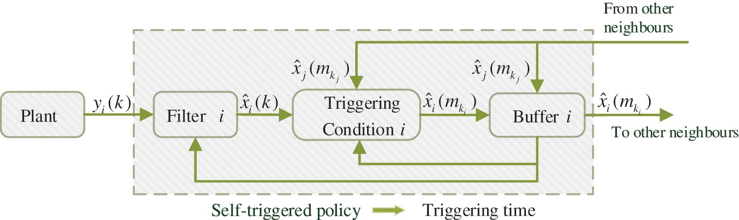
Figure 1: Block diagram of distributed self-triggered system

The self-triggered policy predicts the subsequent execution time and calculates the triggering interval by the latest data of each filter without a continuous judgment process. Therefore, the strategy proposed in this paper is beneficial to the energy saving of sensor networks with limited resources, as well as scant network channel bandwidth.

The self-triggered time-sequence diagram is illustrated in Fig. 2. The dash lines indicate that data is exchanged between nodes and the arrow points to the object of data transmission. The broadcasting and receiving of the latest released state estimation are determined by the filter node’s own self-triggered policy. It is clear that each filter node has its own triggering time sequence, which causes different triggering intervals between each other. Moreover, for filter i, the time that data packets from neighbors arrive at buffer i may be asynchronous, since it is determined by different triggering conditions. Such an asynchronous transmission brings challenges to the design of consensus distributed filtering.

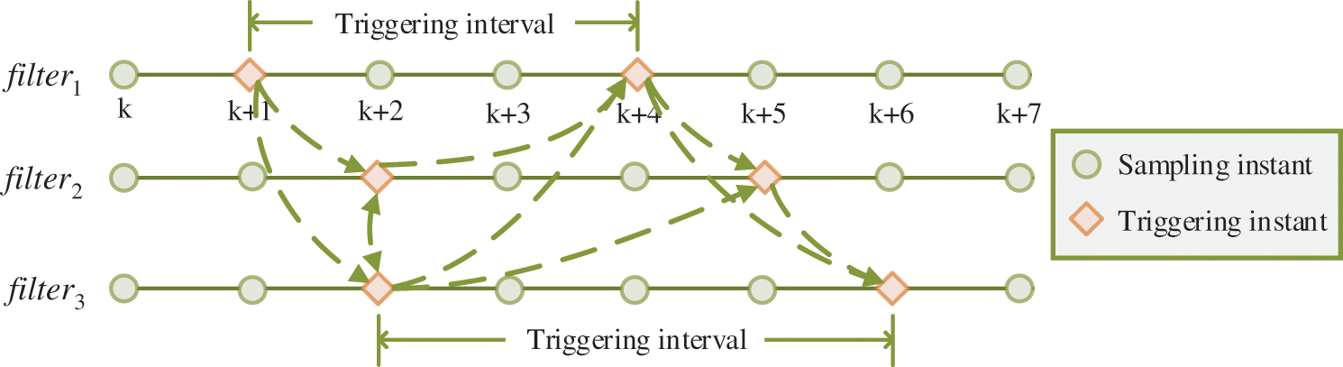
Figure 2: Self-triggered sequence diagram

For filter i, let’s define a state estimation error ei(k)=x(k)−x^i(k), an output estimation error z~i(k)=z(k)−z^i(k) and a state estimation update error e~i(k)=x^i(mki)−x^i(k), k∈[mki,m(k+1)i). Then x^i(mki)−x^j(mkj) can be expressed as e~i(k)−e~j(k)−(ei(k)−ej(k)). Combing (1)–(3), the estimation error dynamics can be rewritten as

{ei(k+1)=(A−HiCi)ei(k)+Bw(k)−HiDivi(k)               +∑j∈NiGi(ei(k)−ej(k))−∑j∈NiGi(e~i(k)−e~j(k))z~i(k)=Mei(k).(4)

The topology of the sensor is determined by a given graph G=(V,E,A). For the sake of brevity, we denote

e(k)=vecnT{eiT(k)}, z˜(k)=vecnT{ z˜iT(k) }, e~(k)=vecnT{e~iT(k)},

v(k)=vecnT{viT(k)}, B¯=vecnT{BT}, M¯=diagn{M},

A¯=diagn{A}, C¯=diagn{Ci}, D¯=diagn{Di}, G¯=diagn{Gi}, H¯=diagn{Hi}.

Then, the error dynamics governed by (4) can be rewritten in the following compact form:

{e(k)=A~e(k)+B~e~(k)+C~v(k)+D~w(k)z~(k)=M¯e(k).(5)

where A~=A¯−H¯C¯+G¯L¯, B~=−G¯L¯, C~=−H¯D¯, D~=B¯ and L¯=L⊗Ip.

Definition 1 ([27]): Filters (3) are said to be a distributed self-triggered H∞ consensus filtering system (1) if they meet the following conditions:

1) In the absence of system disturbance and measurement noise, the filtering error system (5) is exponentially stable, i.e., there exist positive constants η and α∈(0,1) such that limk→∞||e(k)||2≤ηαk, for all k≥0.

2) Under the condition of the system disturbance and measurement noises, the output filtering errors z~i(k),∀i∈V satisfy the following H∞ performance:

1n∑i=1n∑k=0∞‖z~i(k)‖22≤γ2(1n∑i=1n∑k=0∞‖vi(k)‖22+∑k=0∞‖w(k)‖2+1n∑i=1neiT(0)Riei(0))(6)

where γ>0 is the attenuation level and Ri=RiT>0 are some given positive definite matrices.

3  Main Results

In this section, we first design a distributed self-triggered policy. Based on such a policy, sufficient conditions are given for the H∞ consensus analysis of the filtering error system (4). Furthermore, a co-design method for self-triggered threshold parameters and distributed filter gains is presented.

3.1 Self-Triggered Policy

The self-triggered policy predicts that the subsequent execution time depends on the current sampling data and the estimated state updated by its neighbors. Based on this idea, we develop self-triggered distributed filtering. The next triggering instant is considered as follows:

m(k+1)i=mki+Mki(x^i(mki),x^j(mkj),yi(k)).(7)

The key to realizing the self-triggered policy is to obtain the triggering interval function Mki(⋅). We develop the following error-based self-triggered policy:

Mki=inf{(m(k+1)i−mki)∈N|e~iT(k)Φie~i(k)≥εiδiΦiδi}(8)

where δi=∑j∈Niaij(x^i(mki)−x^j(mkj)); εi∈(0,1] is the threshold parameter; Φi∈Rp×p is the weighting matrix to be determined.

Theorem 1: In order to formulate a suitable self-triggered policy for the distributed filtering system (5), the triggering interval function can be expressed as

Mki=m(k+1)i−mki=⌊ln⁡(Q1i(Si−Ui)Q2i+1)/ln⁡(Q1i+1)⌋(9)

where ⌊⋅⌋ denotes rounding up to the nearest integer,

Q1i=‖Φi(I−A+HiCi)Φi−1‖,

Q2i=‖Φi(I−A+HiCi)x^i(mki)‖+‖ΦiGi∑j∈Ni(x^i(mki)−x^j(mkj))‖,

Q3i=‖ΦiHi‖,

Si=‖εiΦiδi‖,

Ui=∑ξ=0k−mki−1(Q1i+1)ξQ3i‖y(k−1−ξ)‖.

Proof: Combining relations (3) and (4), we can obtain

‖Φie~i(k+1)‖−‖Φie~i(k)‖

≤‖Φi(e~i(k+1)−e~i(k))‖

=‖Φi(x^i(k)−x^i(k+1))‖

≤‖Φi(I−A+HiCi)(x^i(mki)−e~i(k))‖+‖ΦiHiyi(k)‖+‖ΦiGi∑j∈Ni(x^i(mki)−x^j(mkj))‖.

≤Q1i‖Φie~i(k)‖+Q2i+Q3i‖yi(k)‖.(10)

Assume Yi(k)=||Φie~i(k)|| Then inequality (10) can be rewritten as

Yi(k+1)−Yi(k)≤Q1iYi(k)+Q2i+Q3i‖yi(k)‖.(11)

From (11), we can obtain

Yi(k)≤(1+Q1i)Yi(k−1)+Q2i+Q3i‖yi(k−1)‖≤(1+Q1i)2Yi(k−2)+(1+Q1i)Q2i+Q2i+(1+Q1i)Q3i‖yi(k−2)‖+Q3i‖yi(k−1)‖⋮≤(1+Q1i)k−mkiYi(mki)+(1+Q1i)k−mki−1Q2i+…+(1+Q1i)Q2i+Q2i+(1+Q1i)k−mki−1Q3i‖yi(mki)‖+…+(1+Q1i)Q3i‖yi(k−2)‖+Q3i‖yi(k−1)‖.(12)

Because Yi(mki)=||Φie~i(mki)||=0 and the right part of (12) is a geometric series, the above inequality could be rewritten as

Yi(k)≤(Q1i+1)k−mki−1Q1iQ2i+∑ξ=0k−mki−1(Q1i+1)ξQ3i‖y(k−1−ξ)‖.(13)

According to self-triggered condition (8), if the filter node i is triggered, the following inequality is obtained

Yi(k)≥‖εiΦiδi‖.(14)

Combining inequality (13) and (14), we have

(1−(Q1i+1)k−mki)Q2i≥(Si−Ui)Q1i.(15)

Through the simple mathematical manipulation of (15), triggering interval (9) is derived.

To guarantee the system performance, the current state estimation of the filter node i should be broadcasted to other neighbors immediately once the triggering conditions are satisfied. This means that the triggering interval Mki should be rounded up. The proof is completed.

3.2 H∞ Consensus Performance Analysis

Lemma 1: Given a positive definite matrix Ri=RiT>0(1≤i≤n), the filtering error system (4) is exponentially stable and satisfy H∞ consensus performance under the self-triggered policy (9) and the initial condition ei(0)TPiei(0)≤γ2ei(0)TRiei(0), if there exist a positive scalar γ>0 and real symmetric matrices Pi>0, Φ¯i satisfying

[Ξ11Ξ1200(PA¯−PH¯C¯+PG¯L¯)T∗Ξ2200(−PG¯L¯)T∗∗−γ2I0(−PH¯D¯)T∗∗∗−nγ2IPB¯T∗∗∗∗−P]≤0(16)

where Ξ11=−P+M¯TM¯+L¯Tε¯Φ¯L¯, Ξ12=−L¯Tε¯Φ¯L¯, Ξ22=L¯Tε¯Φ¯L¯−Φ¯, ε¯i=εi⊗Ip, ε¯=diagn{ε¯i}, Φ¯i=Φi⊗Ip, Φ¯=diagn{Φ¯i}, and P=diagn{Pi}.

Proof: Consider a Lyapunov function

V(k)=e(k)TPe(k).(17)

The one-step time difference is

V(k+1)−V(k)=eT(k+1)Pe(k+1)−eT(k)Pe(k).(18)

According to the self-triggered policy (9), the following inequality in augmented form is valid for [mki,m(k+1)i)

[e(k)e~(k)]TΨ[e(k)e~(k)]≥0(19)

where Ψ is a real symmetric matrix, Ψ11=L¯Tε¯Φ¯L¯, Ψ12=−L¯Tε¯Φ¯L¯, Ψ22= L¯Tε¯Φ¯L¯−Φ¯, and others are zero matrices.

Therefore, Eq. (18) can be rewritten into the following inequality

V(k+1)−V(k)+‖z~(k)‖2−nγ2‖w(k)‖2−γ2‖v(k)‖2≤ξTρTPρξ+ξTΠξ(20)

where ξT=[eT(k),e~T(k),vT(k),wT(k)], ρT=[A~T(k),B~T(k),C~T(k),D~T(k)], Π11=−P+M¯TM¯+L¯Tε¯Φ¯L¯, Π12=−L¯Tε¯Φ¯L¯, Π22=L¯Tε¯Φ¯L¯−Φ¯, Π33=−γ2I, Π44=−nγ2I, and others are zero matrices.

We assume that

Γ≜ρTPρ+Π≤0.(21)

By applying Schur complement lemma to (20), we obtain

Γ=[ΠΥT∗−P]≤0(22)

where Υ=Pρ=[PA¯−PH¯C¯+PG¯L¯,−PG¯L¯,−PH¯D¯,PB¯].

First, we prove that the system (4) is exponentially stable when there is no disturbance and measurement noises. Denoting λ1=λmax(Γ), obviously λ1 is smaller than zero, which indicates that (20) satisfies

V(k+1)−V(k)+‖z~(k)‖2−nγ2‖w(k)‖2−γ2‖v(k)‖2≤λ1‖ξ(k)‖2≤λ1‖e(k)‖2(23)

Define λ2=λmax(P)>0. Then given positive scalar μ, from inequality (23), we obtain

1μk+1v(k+1)−1μk+1v(k)≤λ1μk+1‖e(k)‖2.(24)

With some simple mathematical managements, we get

1μk+1v(k+1)−1μkv(k)≤1μk[λ1μk+(1μk−1)λ2]‖e(k)‖2.(25)

Since 1μk[λ1μk+(1μk−1)λ2]=λ1<0, when μ=1, there exist a constant μ0∈(0,1) such that 1μ0k[λ1μ0k+(1μ0k−1)λ2]<0. By iteration of (25), we have

‖e(k)‖2<λ2λ3μ0k‖e(0)‖2(26)

where λ3=λmin(P)>0. When k approaches to infinity, we can obtain limk→∞||e(k)||2=0 which implies estimation error system (4) is exponentially stable.

Second, it follows from (20) and (21) that

V(k+1)−V(k)≤nγ2‖w(k)‖2+γ2‖v(k)‖2−‖z~(k)‖2(27)

Summing up both sides of (27) from 0 to t with respect to k

∑k=0t‖z~(k)‖22≤nγ2∑k=0t‖w(k)‖2+γ2∑k=0t‖v(k)‖22+V(0)−V(k+1).(28)

Since V(k+1)≥0, letting t approaches to infinity, we can obtain

∑k=0∞‖z~(k)‖22≤nγ2∑k=0∞‖w(k)‖2+γ2∑k=0∞‖v(k)‖22+γ2e(0)TRe(0).(29)

Therefore, the filtering error system also satisfies the H∞ filtering performance condition in Definition 1. The proof is completed.

3.3 Co-Design of Self-Triggered Policy and Asynchronous Distributed Filter

The above Theorem and Lemma will be employed to design distributed self-triggered consensus filtering network (3), which leads to the following theorem.

Theorem 2: Given a positive definite matrix Ri=RiT>0(1≤i≤n), the distributed self-triggered filtering problem is solvable, if there exist a positive scalar γ>0, real symmetric matrices Pi=PiT>0, Φ¯i, and real matrices Xi, Yi satisfying

initial conditions

∑i=1nei(0)TPiei(0)≤γ2∑i=1nei(0)TRiei(0)(30)

and the following set of linear matrix inequalities

[Ξ11Ξ1200(PA¯−XC¯+YL¯)T∗Ξ2200(−YL¯)T∗∗−γ2I0(XD¯)T∗∗∗−nγ2I(PB¯)T∗∗∗∗−P]≤0(31)

where X=diagni{Xi}, Y=diagni{Yi}.

Moreover, if the set of linear matrix inequalities (31) with (30) is feasible, the filter gains can be computed as

Hi=Pi−1Xi,Gi=Pi−1Yi.(32)

Proof: Denoting Xi=PiHi, Yi=PiGi. Then we have

PH¯=X,PG¯=Y.(33)

Substituting relations (33) into inequality (16), it can be seen that the inequality (16) in Lemma 1 results in inequality (31) with (30). The proof is completed.

Remark 1: The goal of the above co-design is to conquer the asynchronous communication caused by self-triggered policy and achieve good filtering performance. Through Theorem 2, the self-triggered threshold parameters Φi and the filter gain matrices Hi, Gi could be successfully solved together.

4  Numerical Example

In this section, a numerical example is given to demonstrate effectiveness of the above co-design.

The network topology is represented by directed weighted graph G=(V,E,A) with five nodes V={1,2,3,4,5}, set of edges E⊆{(1,1),(1,2),(1,3),(1,4),(2,2),(2,3),(3,2),(3,3),(3,4),(4,1),(4,4),(5,3),(5,5)}. The transmission paths between five nodes in Fig. 3 and adjacency matrix as follows:

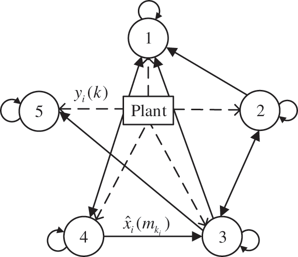
Figure 3: Schematic of distributed filtering over the WSN

A=[1111001100011101001000101].

The simulation is taken as 300-time units and each unit length is taken as 0.1. The system and sensor parameters are given as

A=[ 0.9−0.60.80.3 ], B=[0.51], M=[0.60.6],

C1=[−0.20.3], C2=[−0.30.4], C3=[−0.20.1],

C4=[−0.30.2], C5=[0.2−0.4], D1=D2=D3=D4=[11].

The system noise and measurement noise are taken as ω(k)=e−2k and vi(k)=[e−2ksin⁡(k)2e−kcos⁡(2k)], respectively. The initial state x0=[0.2−0.1]T. The initial estimation of each node i are given as

x^1(0)=[0.2−0.1]T, x^2(0)=[0.2−0.2]T,

x^3(0)=[−0.1−0.2]T, x^4(0)=[0.1−0.2]T, x^5(0)=[0.1−0.1]T.

The self-triggered parameters of each node i are taken as ε1=0.7, ε2=0.2, ε3=0.6, ε4=0.4, ε5=0.3. The positive definite matrices are given R1=R2=R3=R4=R5 =diag2{0.7}.

The self-triggered matrices Φ¯i and the filter gain matrices Hi, Gi are obtained together by solving the linear matrix inequality conditions (30), (31) by the MATLAB software.

To further verify the strength of the self-triggered consensus filtering, a rectangular pulse ωd(k) as an external disturbance is introduced into the system when k∈[8,10]. The simulation results are shown in Figs. 4–6.

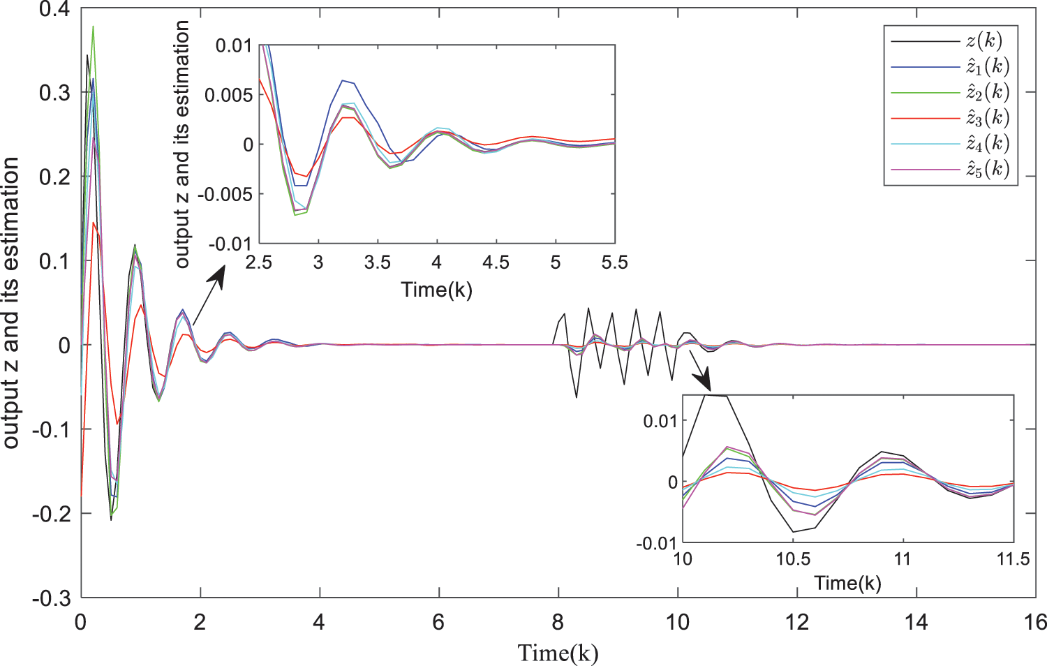
Figure 4: Plant output z(k) and its estimation

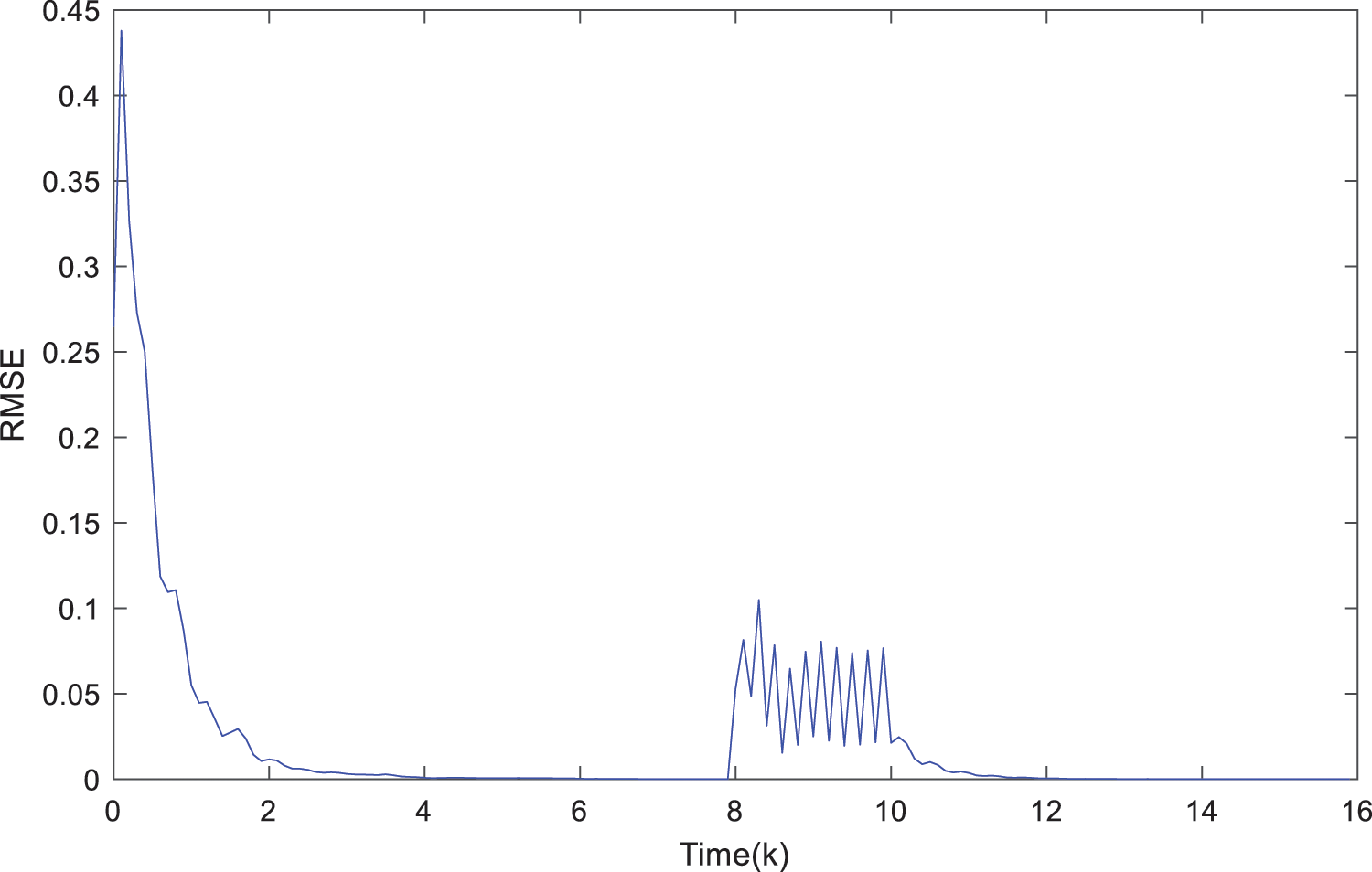
Figure 5: Filtering root mean square error

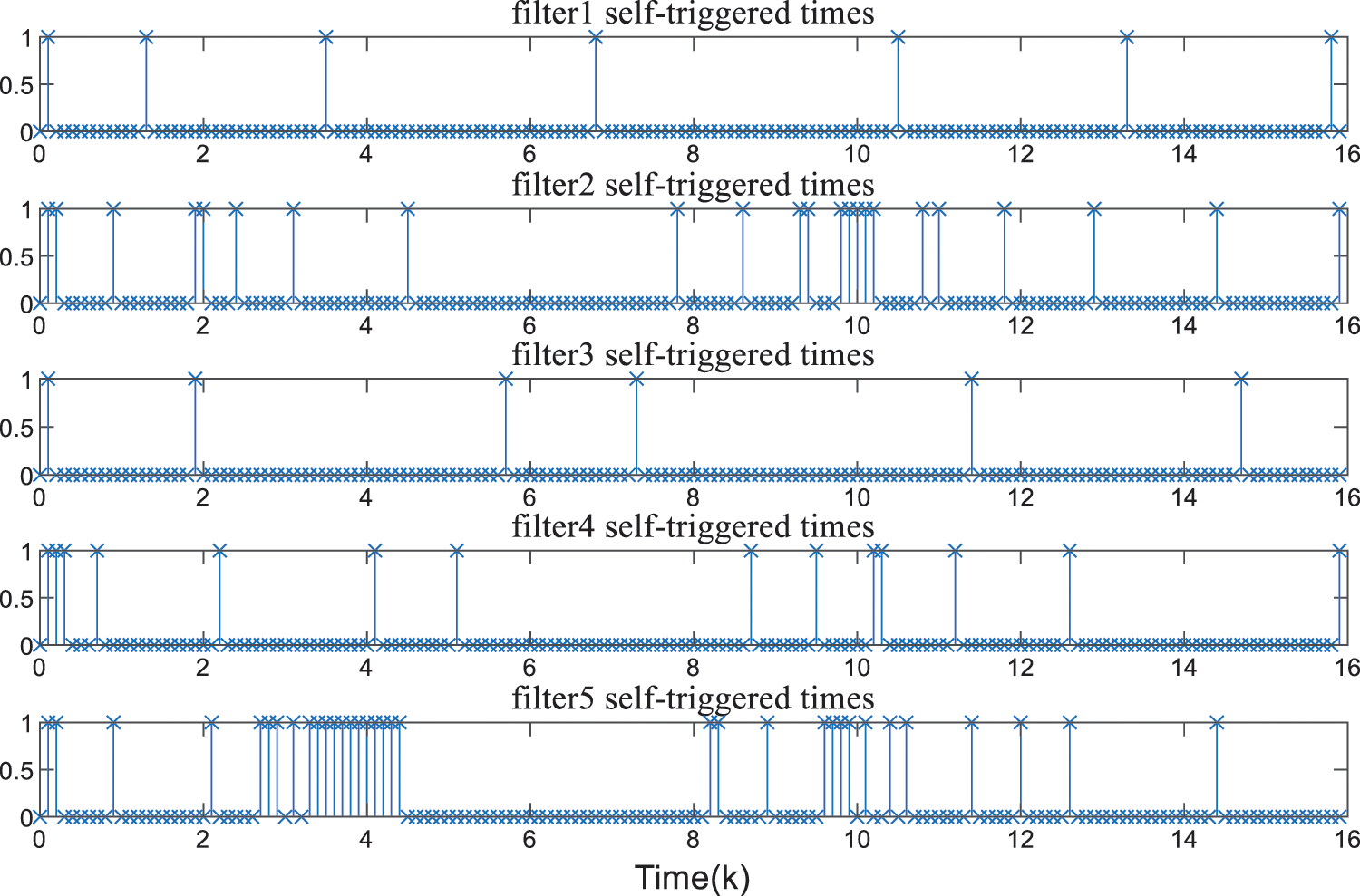
Figure 6: The self-triggered times of each filter

The output z(k) and its estimation are depicted in Fig. 4. The filtering root means square error is given in Fig. 5. They show that the designed self-triggered consensus filter performs well in tracking the state of the target plant and the system has good robustness under the self-triggered policy.

Fig. 6 illustrates the self-triggered times of each filter. Under the periodic time-triggered mechanism, data transmits between the sensor and its neighbors at every sampling moment. It is clear that the self-triggered policy developed in this paper can effectively reduce the data transmission frequency within the network. In particular, in the first 6 time steps, filter 1-filter 5 is triggered less than 20 times under the self-triggered policy, while triggered 60 times under the time-triggered strategy. Therefore, the self-triggered policy developed in this paper can greatly save communication resources and computation burden of the filtering network.

On the other hand, after the system is perturbed, the number of triggers intensively increases, and the triggers become gentle until the estimation becomes consensus during the time interval k∈[8,14]. This also means that filter i should update data released from neighbors frequently when the filtering departs from consistency.

In summary, the simulation results illustrate that the self-triggered policy can save communication and computation burden while satisfying filtering performance.

5  Conclusion

The self-triggering policy is developed for a class of distributed filtering systems in this paper. This policy can actively predict the time when the following exchanged data will be updated. Through such a policy, the frequency of data exchange can be reduced, while communication resources can be saved within the filtering network. Compared with the existing event-triggered communication scheme, this means that it is not necessary to continuously judge trigger conditions, which saves the computing burden. The asynchronous transmission problem caused by each filter node’s independent self-triggering can be solved by co-design. In order to make the research work close to the engineering practice, we will further consider transmission delay, packet loss, data conflicts, and other network induced phenomena.

Funding Statement: This work was jointly supported by the National Natural Science Foundation of China (Nos. 61991402, 62073154), the 111 Project (B12018), the Scientific Research Cooperation and High-Level Personnel Training Programs with New Zealand (1252011004200040).

Conflicts of Interest: The authors declare that they have no conflicts of interest to report regarding the present study.

References

1. Yang, X. S., Zhang, W. A., Yu, L., Xing, K. X. (2016). Multi-rate distributed fusion estimation for sensor network-based target tracking. IEEE Sensor Journal, 16(5), 1233–1242. DOI 10.1109/JSEN.2015.2497464. [Google Scholar] [CrossRef]
2. La, H. M., Sheng, W. H. (2013). Distributed sensor fusion for scalar field mapping using mobile sensor networks. IEEE Transactions on Cybernetics, 43(2), 766–778. DOI 10.1109/TSMCB.2012.2215919. [Google Scholar] [CrossRef]
3. Shen, B., Wang, Z. D., Hung, Y. S. (2010). Distributed H-infinity-consensus filtering in sensor networks with multiple missing measurements: The finite-horizon case. Automatica, 46(10), 7682–7688. DOI 10.1016/j.automatica.2010.06.025. [Google Scholar] [CrossRef]
4. Ding, D., Wang, Z. D., Ho, D. W. C., Wei, G. L. (2017). Distributed recursive filtering for stochastic systems under uniform quantizations and deception attacks through sensor networks. Automatica, 78(1), 231–240. DOI 10.1016/j.automatica.2016.12.026. [Google Scholar] [CrossRef]
5. Ma, L. F., Wang, Z. D., Alsaadi, F. E. (2019). Distributed filtering for nonlinear time-delay systems over sensor networks subject to multiplicative link noises and switching topology. International Journal of Robust and Nonlinear Control, 29(10), 2941–2959. DOI 10.1002/rnc.4535. [Google Scholar] [CrossRef]
6. Liu, Y. R., Wang, Z. D., Liang, J. L., Liu, X. H. (2008). Synchronization and state estimation for discrete-time complex networks with distributed delays. IEEE Transactions on Systems, Man, and Cybernetics, Part B (Cybernetics), 38(5), 1314–1325. DOI 10.1109/TSMCB.2008.925745. [Google Scholar] [CrossRef]
7. Liu, Q. Y., Wang, Z. D., He, X., Zhou, D. H. (2015). Event-based distributed filtering with stochastic measurement fading. IEEE Transactions on Industrial Informatics, 11(6), 1643–1652. DOI 10.1109/TII.2015.2444355. [Google Scholar] [CrossRef]
8. Zhang, X. M., Han, Q. L., Ge, X. H., Ding, D. R., Ding, L. et al. (2020). Networked control systems: A survey of trends and techniques. IEEE/CAA Journal of Automatica Sinica, 7(1), 1–17. DOI 10.1109/JAS.2019.1911651. [Google Scholar] [CrossRef]
9. Wang, X., Su, H. S. (2019). Self-triggered leader-following consensus of multi-agent systems with input time delay. Neurocomputing, 330(9), 70–77. DOI 10.1016/j.neucom.2018.10.077. [Google Scholar] [CrossRef]
10. Wang, M., Wang, Z. D., Chen, Y., Sheng, W. G. (2019). Event-based adaptive neural tracking control for discrete-time stochastic nonlinear systems: A triggering-threshold compensation strategy. IEEE Transactions on Neural Networks and Learning Systems, 31(6), 1968–1981. DOI 10.1109/TNNLS.2019.2927595. [Google Scholar] [CrossRef]
11. Li, B., Wang, Z. D., Ma, L. F., Liu, H. J. (2019). Observer-based event-triggered control for nonlinear systems with mixed delays and disturbances: The input-to-state stability. IEEE Transactions on Cybernetics, 49(7), 2806–2819. DOI 10.1109/TCYB.2018.2837626. [Google Scholar] [CrossRef]
12. Ma, L. F., Wang, Z. D., Lam, H. K., Kyriakoulis, N. (2017). Distributed event-based set-membership filtering for a class of nonlinear systems with sensor saturations over sensor networks. IEEE Transactions on Cybernetis, 47(11), 3772–3783. DOI 10.1109/TCYB.2016.2582081. [Google Scholar] [CrossRef]
13. Su, H. S., Li, Z. H., Ye, Y. Y. (2017). Event-triggered Kalman-consensus filter for two-target tracking sensor networks. ISA Transactions, 71(1), 103–111. DOI 10.1016/j.isatra.2017.06.019. [Google Scholar] [CrossRef]
14. Muehlebach, M., Trimpe, S. (2018). Distributed event-based state estimation for networked systems: An LMI approach. IEEE Transactions on Automatic Control, 63(1), 269–277. DOI 10.1109/TAC.2017.2726002. [Google Scholar] [CrossRef]
15. Wang, L. C., Wang, Z. D., Han, Q. L., Wei, G. (2018). Event-based variance-constrained H-infinity filtering for stochastic parameter systems over sensor networks with successive missing measurements. IEEE Transactions on Cybernetis, 48(3), 1007–1017. DOI 10.1109/TCYB.2017.2671032. [Google Scholar] [CrossRef]
16. Hu, J., Wang, Z. D., Liang, J. L., Dong, H. L. (2015). Event-triggered distributed state estimation with randomly occurring uncertainties and nonlinearities over sensor networks: A delay-fractioning approach. Journal of the Franklin Institute, 352(9), 3750–3763. DOI 10.1016/j.jfranklin.2014.12.006. [Google Scholar] [CrossRef]
17. Gu, Z., Zhou, X. H., Zhang, T., Yang, F., Shen, M. Q. (2020). Event-triggered filter design for nonlinear cyber-physical systems subject to deception attacks. ISA Transactions, 104(3), 130–137. DOI 10.1016/j.isatra.2019.02.036. [Google Scholar] [CrossRef]
18. Ge, X. H., Han, Q. L., Wang, Z. D. (2019). A threshold-parameter-dependent approach to designing distributed event-triggered H-infinity-consensus filters over sensor networks. IEEE Transactions on Cybernetics, 49(4), 1148–1159. DOI 10.1109/TCYB.2017.2789296. [Google Scholar] [CrossRef]
19. Xiao, S. Y., Han, Q. L., Ge, X. H., Zhang, Y. J. (2020). Secure distributed finite-time filtering for positive systems over sensor networks under deception attacks. IEEE Transactions on Cybernetics, 50(3), 1220–1229. DOI 10.1109/TCYB.2019.2900478. [Google Scholar] [CrossRef]
20. Ding, L., Guo, G. (2015). Distributed event-triggered H-infinity consensus filtering in sensor networks. Signal Processing, 108(3), 365–375. DOI 10.1016/j.sigpro.2014.09.035. [Google Scholar] [CrossRef]
21. Xia, N., Yang, F. W., Han, Q. L. (2017). Distributed event-triggered networked set-membership filtering with partial information transmission. IET Control Theory and Applications, 11(2), 155–163. DOI 10.1049/iet-cta.2016.0781. [Google Scholar] [CrossRef]
22. Zhang, H., Wang, Z. P., Yan, H. C., Yang, F. W., Zhou, X. (2019). Adaptive event-triggered transmission scheme and H-infinity filtering co-design over a filtering network with switching topology. IEEE Transactions on Cybernetics, 49(12), 4296–4307. DOI 10.1109/TCYB.2018.2862828. [Google Scholar] [CrossRef]
23. Ge, X. H., Han, Q. L., Wang, Z. D. (2019). A dynamic event-triggered transmission scheme for distributed set-membership estimation over wireless sensor networks. IEEE Transactions on Cybernetics, 49(1), 171–183. DOI 10.1109/TCYB.2017.2769722. [Google Scholar] [CrossRef]
24. Zhang, H., Hong, Q. Q., Yan, H. C., Yang, F. W., Guo, G. (2017). Event-based distributed H-infinity filtering networks of 2-DOF quarter-car suspension systems. IEEE Transactions on Industrial Informatics, 13(1), 312–321. DOI 10.1109/TII.2016.2569566. [Google Scholar] [CrossRef]
25. Velasco, M., Fuertes, J., Marti, P. (2003). The self-triggered task model for real-time control systems. Work-in-Progress Session of the 24th IEEE Real-Time Systems Symposium (RTSS03), vol. 384, pp. 67–70. [Google Scholar]
26. Fan, Y., Liu, L., Feng, G., Wang, Y. (2015). Self-triggered consensus for multi-agent systems with Zeno-free triggers. IEEE Transactions on Automatic Control, 60(10), 2779–2784. DOI 10.1109/TAC.2015.2405294. [Google Scholar] [CrossRef]
27. Heemels, W. P. M. H., Johansson, K. H., Tabuada, P. (2012). An introduction to event-triggered and self-triggered control. 51st IEEE Conference on Decision and Control (CDC), pp. 3270–3285. Maui, HI, USA. DOI 10.1109/CDC.2012.6425820 [Google Scholar] [CrossRef]
28. Dimarogonas, D. V., Frazzoli, E., Johansson, K. H. (2012). Distributed event-triggered control for multi-agent systems. IEEE Transactions on Cybernetics, 57(5), 1291–1297. DOI 10.1109/TAC.2011.2174666. [Google Scholar] [CrossRef]
29. Ding, L., Han, Q. L., Ge, X., Zhang, X. M. (2018). An overview of recent advances in event-triggered consensus of multiagent systems. IEEE Transactions on Cybernetics, 48(4), 1110–1123. DOI 10.1109/TCYB.2017.2771560. [Google Scholar] [CrossRef]
30. Liu, C. X., Li, H. P., Gao, J., Xu, D. (2018). Robust self-triggered min-max model predictive control for discrete-time nonlinear systems. Automatica, 89(6), 333–339. DOI 10.1016/j.automatica.2017.12.034. [Google Scholar] [CrossRef]
31. Wan, H. Y., Luan, X. L., Karimi, H. R., Liu, F. (2021). Dynamic self-triggered controller codesign for Markov jump systems. IEEE Transactions on Automatic Control, 66(3), 1353–1360. DOI 10.1109/TAC.2020.2992564. [Google Scholar] [CrossRef]
32. Yang, H., Wang, Z. D., Shen, Y. X., Alsaadi, F. E. (2021). Self-triggered filter design for a class of nonlinear stochastic systems with Markovian jumping parameter. Nonlinear Analysis-Hybrid Systems, 40(1), 101022. DOI 10.1016/j.nahs.2021.101022. [Google Scholar] [CrossRef]
Cite This Article
Copyright © 2023 The Author(s). Published by Tech Science Press.
This work is licensed under a Creative Commons Attribution 4.0 International License , which permits unrestricted use, distribution, and reproduction in any medium, provided the original work is properly cited.
Downloads
Citation Tools