
 Submit a Paper
 Propose a Special lssue
 Open Access
ARTICLE
Numerical Assessment of Nanofluid Natural Convection Using Local RBF Method Coupled with an Artificial Compressibility Model
1 Department of Mathematics and Statistics, College of Science, King Faisal University, Al-Ahsa, 31982, Saudi Arabia
2 PTPME Laboratoy, Faculty of Sciences, Mohamed First University, Oujda, 60000, Morocco
* Corresponding Author: Muneerah Al Nuwairan. Email:
Computer Modeling in Engineering & Sciences 2023, 135(1), 133-154. https://doi.org/10.32604/cmes.2022.022649
Received 18 March 2022; Accepted 25 May 2022; Issue published 29 September 2022
 View Full Text
 Download PDF
Abstract
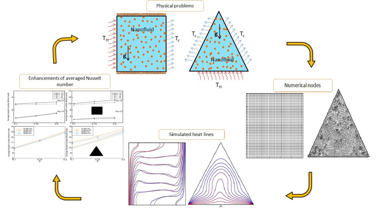
In this paper, natural heat convection inside square and equilateral triangular cavities was studied using a meshless method based on collocation local radial basis function (RBF). The nanofluids used were Cu-water or -water mixture with nanoparticle volume fractions range of . A system of continuity, momentum, and energy partial differential equations was used in modeling the flow and temperature behavior of the fluids. Partial derivatives in the governing equations were approximated using the RBF method. The artificial compressibility model was implemented to overcome the pressure velocity coupling problem that occurs in such equations. The main goal of this work was to present a simple and efficient method to deal with complex geometries for a variety of problem conditions. To assess the accuracy of the proposed method, several test cases of natural convection in square and triangular cavities were selected. For Rayleigh numbers ranging from to , a validation test of natural convection of Cu-water in a square cavity was used. The numerical investigation was then extended to Rayleigh number , as well as -water nanofluid with a volume fraction range of . In a second investigation, the same nanofluids were used in a triangular cavity with varying volume fractions to test the proposed meshless approach on non-rectangular geometries. The numerical results appear to be in agreement with those from earlier investigations. Furthermore, the suggested meshless method was found to be stable and accurate, demonstrating that it may be a viable alternative for solving natural heat transfer equations of nanofluids in enclosures with irregular geometries.Graphic Abstract
Keywords
Abbreviations
| N | Number of nodes |
| Cp | Specific heat, |
| g | Acceleration due to gravity, |
| k | Thermal conductivity, |
| Nu | Nusselt number |
| Pr | Prandtl number |
| Ra | Rayleigh number |
| p | Pressure, |
| P | Dimensionless pressure |
| T | Temperature, |
| Dimensionless temperature | |
| u, v | Dimensional velocity components in x and y, |
| U, V | Dimensionless velocity components in X and Y |
| x, y | Dimensional Cartesian coordinates |
| X, Y | Dimensionless Cartesian coordinates |
| First-order differentiation matrix | |
| Second-order differentiation matrix | |
| Greek Symbols | |
| thermal diffusivity, | |
| thermal expansion coefficient, | |
| effective viscosity, | |
| density, | |
| artificial compressibility parameter | |
| shape parameter | |
| pseudo time | |
| Subscripts | |
| f | base fluid |
| nf | nanofluid |
| p | solid particles |
| c | cold |
| h | hot |
In heat transfer, the heat convection occurs when heat is transferred from one part of the fluid to another. Natural convection has become an active research topic due to its lower cost and wide applications in engineering. Several models were developed for calculating the efficiency of thermal conductivity in solid and fluid systems [1–6]. In [7], Choi showed that adding some nano metal particles to the base fluid increases its conductivity. Such mixtures, known as nanofluids, have many applications in science and engineering [8]. These applications include fuel cells, hybrid-powered engines, chillers, and heat exchangers. The usefulness of a nanofluid for heat transfer applications can be verified by modeling the convective transfer in the nanofluid.
Several numerical methods, such as finite elements, finite volumes, and finite differences have been used to solve the thermal convection equations and simulate convective heat flow in various geometries. These methods are mesh based methods and are widely used. Several researchers have used these methods to model natural convection in nanofluids. Oztop et al. [9] used the method of finite volumes to investigate thermal transfer in a square cavity filled with a nanofluid. The investigation examined the effect of the size of the nanoparticles and the type of nanofluid. Mahmoodi et al. [10] used the same method with the SIMPLER algorithm to investigate heat transfer in a square cavity filled with nanofluid and having adiabatic square bodies at its center. These two studies found that increasing the volume fraction of the nanofluid increases heat transfer and that the type of nanoparticle is a key factor in heat transfer improvement. Jasim et al. [11] studied the influence of an inner adiabatic rotating cylinder on mixed convection of hybrid nanofluid in more complex geometries. Their research gave important insights for rotary heat exchanger designers. The set of conservation equations and their associated boundary conditions were discretized using the finite volume technique.
Finite elements have also been widely used. For example, Bhowmick et al. [12] used the Galerkin Finite Element Method to discretize the governing equations of natural convection heat transfer and entropy generation for a square enclosure, containing a heated circular or square cylinder subjected to non-uniform temperature distributions on the left vertical and bottom walls. The finite element method was also used by Islam et al. [13] to analyze temperature transfer within a prismatic cavity filled with
It is worth noting that, over the last two decades, the lattice Boltzmann method has seen significant advances and is now commonly used in heat transfer problems, particularly for nanofluids. In Izadi et al. [14], natural convection of multi-wall carbon nanotubes-Iron Oxide nanoparticles/water hybrid nanofluid inside a
Recently, Petrov-Galerkin local meshless method was used to study natural convection in a porous medium [16], Wijayanta et al. [17] analyzed a local radial basis function method to obtain numerical solutions of the conjugate natural convection heat transfer problem for square cavity. Zhang et al. [18] tested the robustness and accuracy of the variational multiscale element free Galerkin method, another meshless method, on several cases of natural convection, including a semicircular cavity, a triangular cavity with a flat wall, and a zigzag shape. The results obtained in these studies clearly showed that meshless methods are stable, accurate, and efficient. In addition to these classic methods, artificial neural networks (ANN) were used in studying convention heat transfer. An ANN based method was developed by Rostami et al. [19] to predict the thermal conductivity of multiwall carbon nanotubes-water and Cu-water nanofluids. Using experimental data, their algorithm selects ANNs with optimal performance on the prediction problem at hand. This study found that ANNs have excellent predictive ability and can make important contributions to the determination of the most desirable performance.
Other lines of investigation relevant to our study were explored. Kavusi et al. [20] studied the effect of different nanofluids, prepared using alumina, copper oxide and silver nanoparticles, at different concentrations and particle diameters on the performance of heat pipe, a heat exchange device with high efficiency and performance in heat transfer. Their study found that the use of a nanofluid in place of water resulted in an increase in thermal efficiency and a reduction in heat at the heat pipe wall. Rahmati et al. [21] simulated heat transfer in a microtube. The cooling fluid used was a combination of 1% and 1.5% volume fractions of CuO nanoparticles in a non-Newtonian pseudo-plastic fluid. Several challenges were identified in this work, namely the effect of slip velocity and the choice of the power law model for dynamic viscosity estimation. This study found that increasing the volume fraction of solid nanoparticles and the slip velocity coefficient resulted in an increase in heat transfer.
The present work aims to develop an accurate method using local radial basis function combined with the artificial compressibility model to solve the natural convective heat transfer problems in complex geometries. These methods have rarely been used in the case of nanofluids. A square cavity and an equilateral triangular cavity filled with a Cu-water or
This paper is structured as follows: The problem and the mathematical implementation of the governing equations are described in Section 2. The numerical formulas of the meshless approach are detailed in Section 3. In Section 4, the numerical method is applied and the numerical results are presented, along with a discussion of the accuracy and efficiency. Section 5 summarizes the results, adding some remarks and conclusions.
2 Problems Definition and Governing Equations
To demonstrate the simplicity and efficiency of the proposed method to deal with complex geometries, we choose two domains. The proposed configurations are illustrated in Fig. 1, they consist of:
• A two-dimensional square cavity. The left and right walls of the square cavity are the hot wall (
• An equilateral triangular cavity where the bottom wall is the hot wall while the other two upper walls are kept adiabatic.
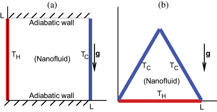
Figure 1: Schematic geometry of physical problems: (a) Differentially heated square cavity and (b) Uniformly heated triangular cavity from bottom
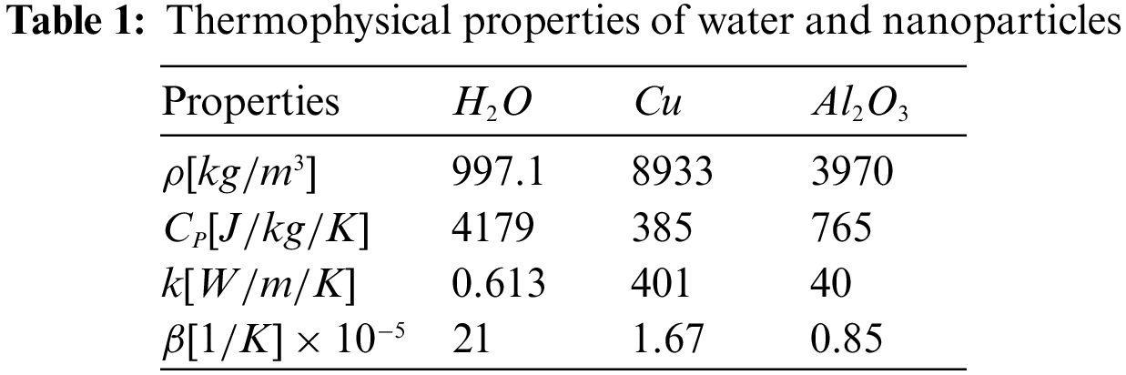
The cavities considered are filled with a nanofluid composed of a nanoparticle-water mixture. The nanofluid is considered Newtonian, and the flow is laminar. The thermo-physical properties of the base fluid and the nanoparticle are taken as [22] and listed in Table 1.They are assumed constant except for the density which is given by the Boussinesq approximation.
The equations of the continuity, momentum, and energy for buoyancy-driven laminar fluid flow and heat transfer of the nanofluid inside a cavity are
where u and v are the components of the velocity in the x and y directions, T is the temperature, p is the pressure, the meaning of the other variables are found in the abbreviations at the end of the paper. Using the dimensionless variables:
L is the characteristic length as well as the length of the cavity edge. For this work, we set it to 1. The above equations can be written in the dimensionless form:
where
For the cases studied, we have used three types of walls; hot, cold or adiabatic wall. The corresponding boundary conditions are
•
•
•
•
For calculating the local and average Nusselt numbers, the following formulas were used, respectively
In this work, the values of the Nusselt number were calculated on horizontal or vertical walls, where for a horizontal wall
2.3 Nanofluid Thermophysical Properties
The thermophysical parameters of the base fluid, such as density, viscosity, and heat conductivity, are affected by the addition of nanoparticles. In this study, the models that describe the thermophysical properties were obtained from the literature and are as follows:
The effective density of the nanofluid is given as
where
where
Here
The thermal expansion coefficient of the nanofluid is given by
Finally, the effective viscosity of the nanofluid, based on Brinkman model [24], is given by:
where
3.1 Radial Basis Function (RBF) Method
We employ the radial basis functions method, which is a meshless method originally proposed by Kansa [25], for the numerical solution of natural convection equations. In the following, we outline the main principles of this method.
Radial basis function interpolation approximates the solution function by an expansion. According to the Kansa method, the solution is approximated on a set of N collocation nodes by a linear combination of local radial basis function as follows [26]:
where
Many radial basis functions were proposed In the literature. In the current study, we use the infinitely smooth multiquadric radial basis function defined as
The numerical solution of an equation involving partial derivatives can be approximated by using linear approximation of the partial derivatives at the
This can be rewritten in a more concise form as
where
where
Note that in the governing equations the first and second derivatives are calculated for each node by using several matrix operations on
Using this approach, the first and second spatial derivatives of a function
where
In attempting a numerical solution of the Eqs. (6)–(9), one is faces with several difficulties. The momentum equations contain a pressure gradient, moreover, these equations can not be solved if the pressure term is not specified. The method of artificial compressibility proposed by Chorin [29] is adopted in this work for the treatment of the pressure-velocity coupling. This method adds a pseudo-temporal derivative to the continuity equation to couple pressure with velocity, as follows:
Here
For simplicity, the Eqs. (25), (7)–(9) are rewritten in a compact form as follows:
where,
with the superscript T denoting the transpose and
On a set of N nodes, and using the differentiation matrix defined above, the right-hand side of the partial differential problem (25) can be approximated as
The problem in Eq. (26) is integrated explicitly using the second Runge-Kutta method. Hence, we divide the pseudo-time into intervals
where
and
It should be noted that radial basis function approaches for time-dependent partial differential equations with diffusive terms can be stably advanced in time with a suitable choice of time step size [27]. Although, the equations used in our study are time dependent, the aim of the study is to examine the steady-state solution. Thus, the method is used to reach the steady-state as the limit when the variations of variables approaches zero. The convergence criteria for steady state is
and
Here n and
3.3 Grid Independence and Validation Tests
Several preliminary tests were performed to evaluate the sensitivity of the results to the number of nodes. These tests were used to determine the optimal distribution of nodes that ensures good accuracy with reasonable computational cost, Three distributions are used for this investigation and are shown in Fig. 2. For these tests Cu-water nanofluid with volume fraction
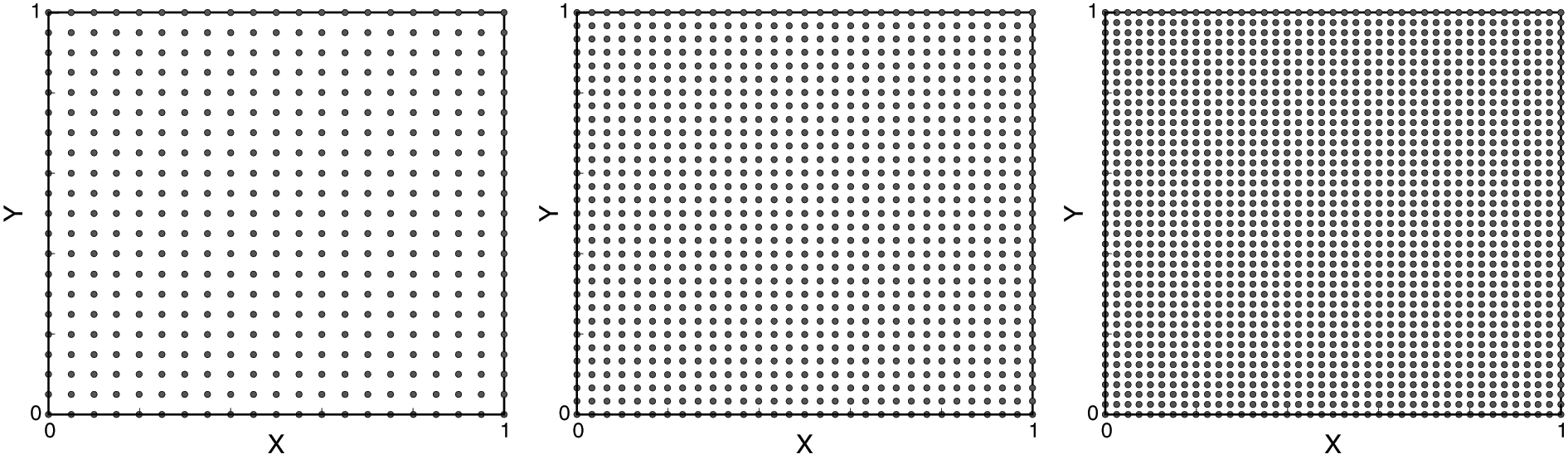
Figure 2: Nodes distribution used for the study of grid independence for square cavity. 21 × 21 to the left, 31 × 31 at the middle and 41 × 41 to the right
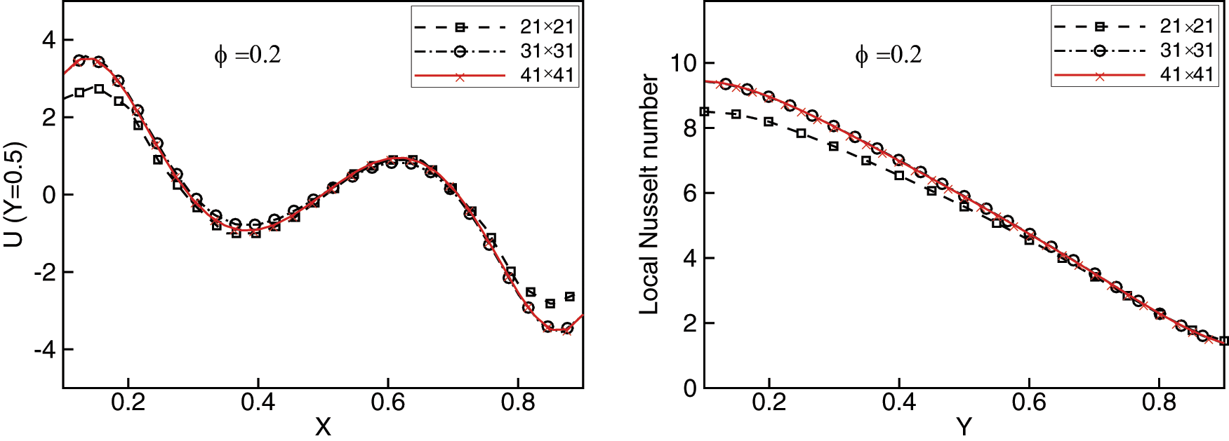
Figure 3: Grid independence tests for variations of the U component of the velocity vs. X coordinate at Y = 0.5 (left) and local Nusselt number vs. Y coordinate at left wall (right)
The meshless method proposed in this work was then validated in the case of natural convection on two problems. The first was the natural convection in a cavity filled with pure water. In the second, we considered the Cu-water nanofluid with a volume fraction
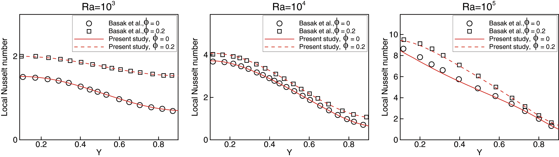
Figure 4: Validation cases in Basak et al. [30] and present study. local Nusselt number vs. Y coordinate at left wall for Ra = 103, 104 and 105 and for Cu-water nanofluid with ϕ = 0.2 and pure water
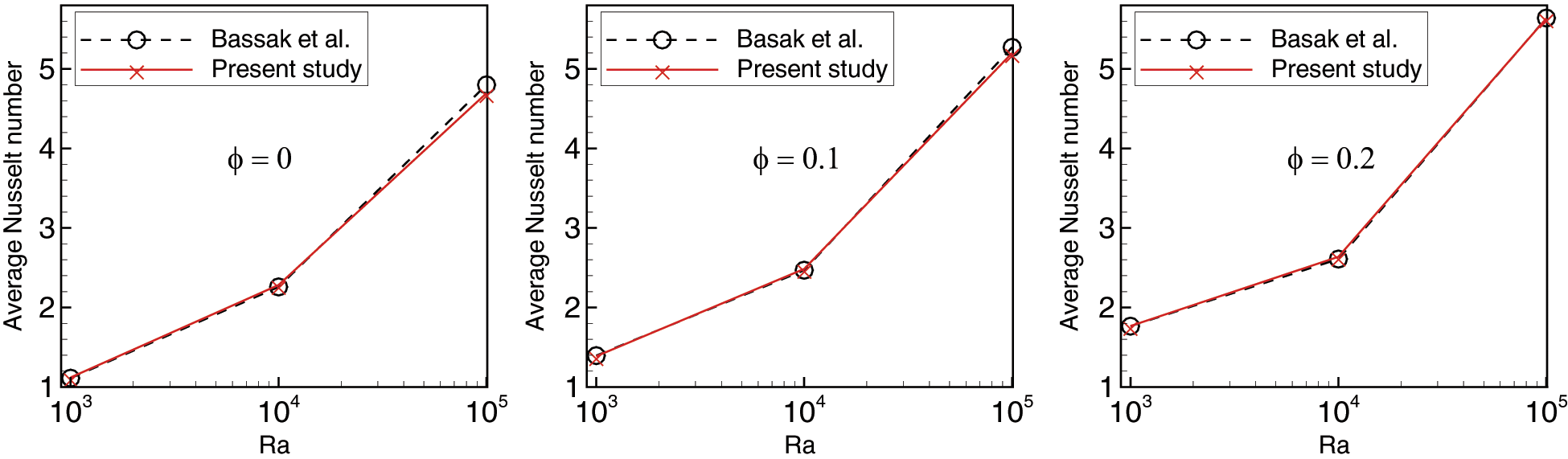
Figure 5: Validation cases in Basak et al. [30] and present study. Average Nusselt number vs. Rayleigh for ϕ = 0 , ϕ = 0.1 and ϕ = 0.2 of Cu-water nanofluid
4.1 Differentially Heated Square Cavity
In the first investigation, we ran a simulation of the effects of differentially heated boundary conditions on natural convection in a square cavity filled with a nanofluid. We used the cavity previously for the validation of meshless method, but extend the range of the Raylieh number to
Figs. 6 and 7 show isotherms distributions for dilute Cu-water and
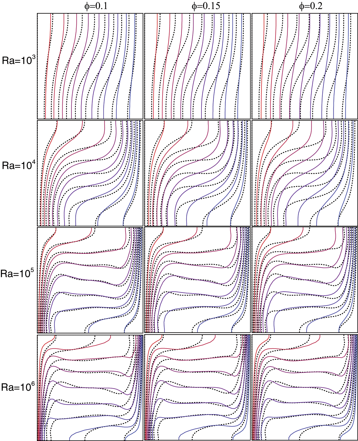
Figure 6: Isotherms of differentially heated square cavity with a hot wall on the left, cold wall on the right, of pure water (dotted line) and a Cu-water nanofluid (continued), for volume fraction ϕ = 0.1, 0.15 and 0.2, and the numbers of Ra = 103, 104, 105 and 106
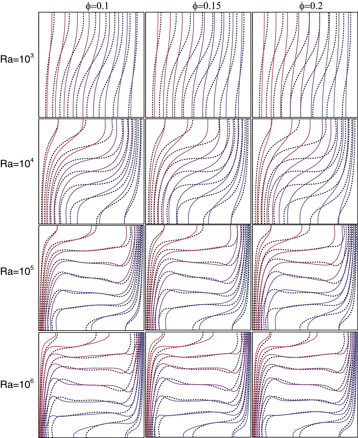
Figure 7: Isotherms of differentially heated square cavity with a hot wall to the left, cold wall to the right, of pure water (dotted line) and a Al2O3-water nanofluid (continued), for volume fraction ϕ = 0.1, 0.15 and 0.2, and the numbers of Ra = 103, 104, 105 and 106
Figs. 8 and 9 illustrate the variations in the local Nusselt number along the heated wall for different values of the Rayleigh number and different volume fractions for the Cu-water and
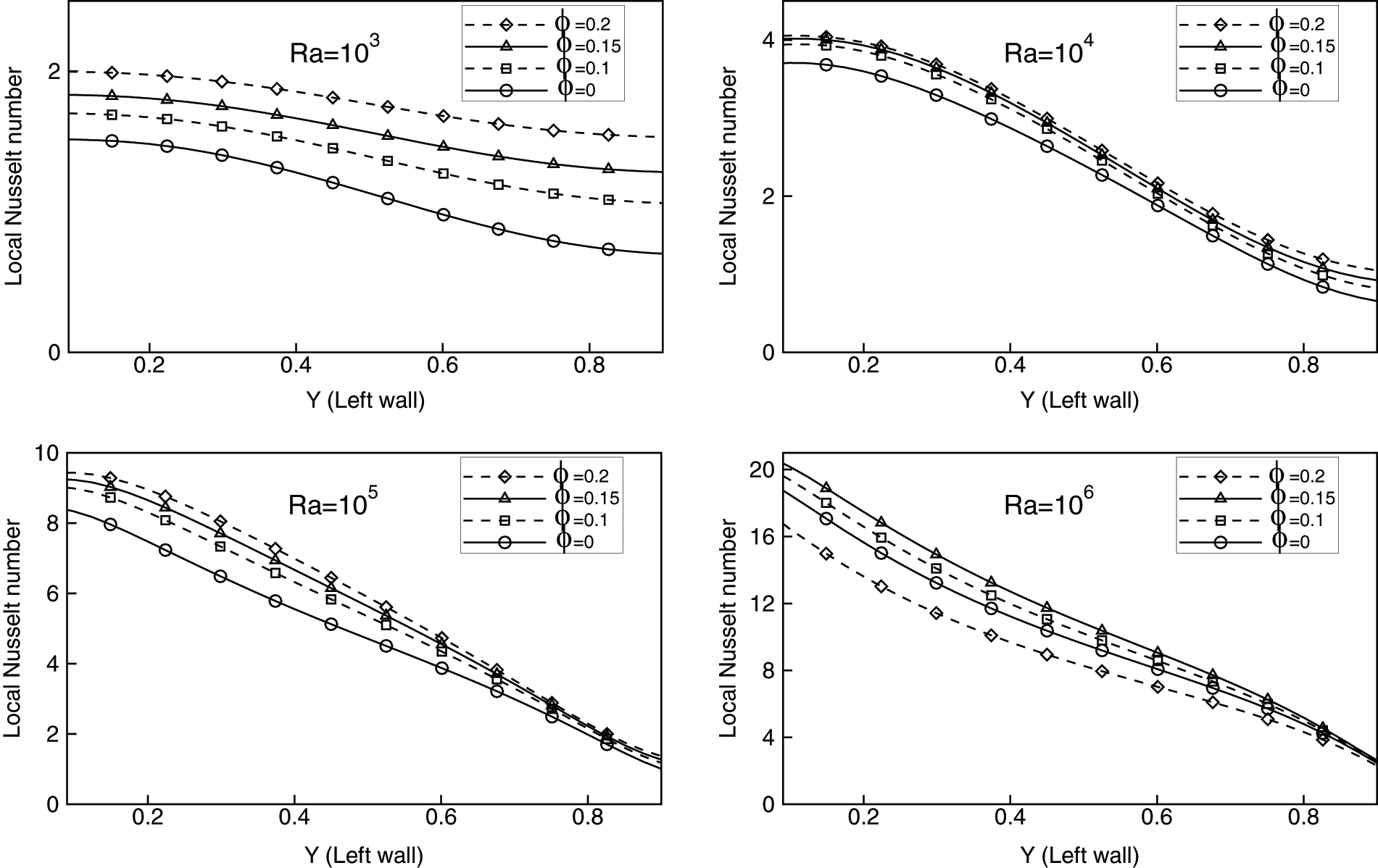
Figure 8: Local Nusselt number at the left wall for Cu-water nanofluid with the volume fractions ϕ = 0, 0.1, 0.15 and 0.2 at Rayleigh numbers 103, 104, 105 and 106
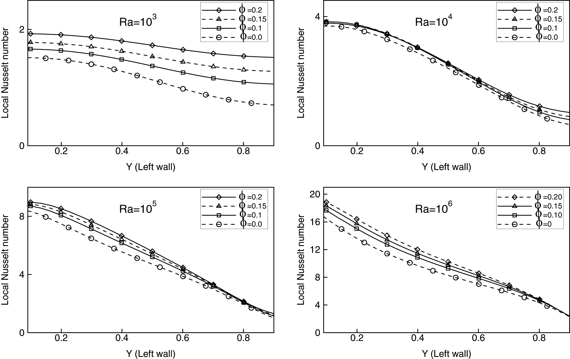
Figure 9: Local Nusselt number at the left wall for Al2O3-water nanofluid with the volume fractions ϕ = 0, 0.1, 0.15 and 0.2 at Rayleigh numbers 103, 104, 105 and 106
Fig. 10 shows the variation of average Nusselt number against nanoparticle volume fraction for
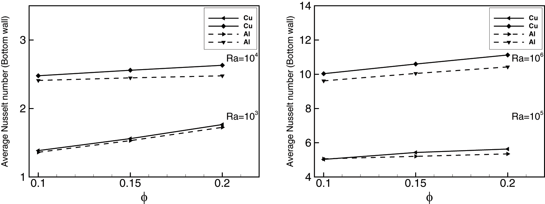
Figure 10: Comparison and variation of average Nusselt number with volume fractions of Cu and Al2O3 nanoparticles at different Rayleigh number
4.2 Uniform Heated Triangular Cavity
In the second investigation, we looked at the natural convection in an equilateral triangular enclosure. The two nanofluids employed in the previous case were used. The two inclined walls of the cavity were kept cold, while the bottom wall is heated. Pranowo et al. [31] used a similar configuration filled with air to test the performance of their meshless method. The nodes distribution used for the numerical computation (Fig. 11) contains 1043 non-uniformly distributed nodes. Figs. 12 and 13 show the impact of Rayleigh number and volume fraction of nanoparticles on isotherms. As expected, for low Rayleigh numbers thermal conduction dominates. For the case of the triangular cavity this dominance occurs at Rayleigh numbers lower than
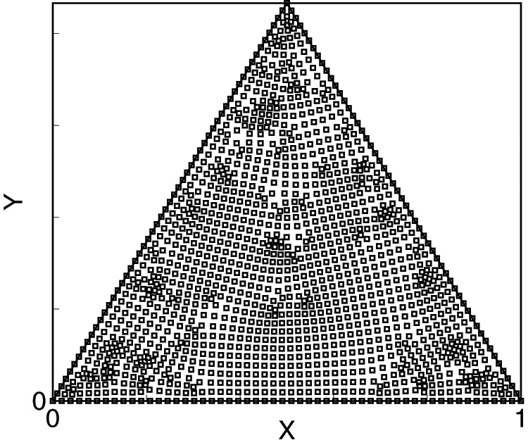
Figure 11: Node distribution used for numerical studies for triangular cavity, 1043 non-uniformly distributed nodes
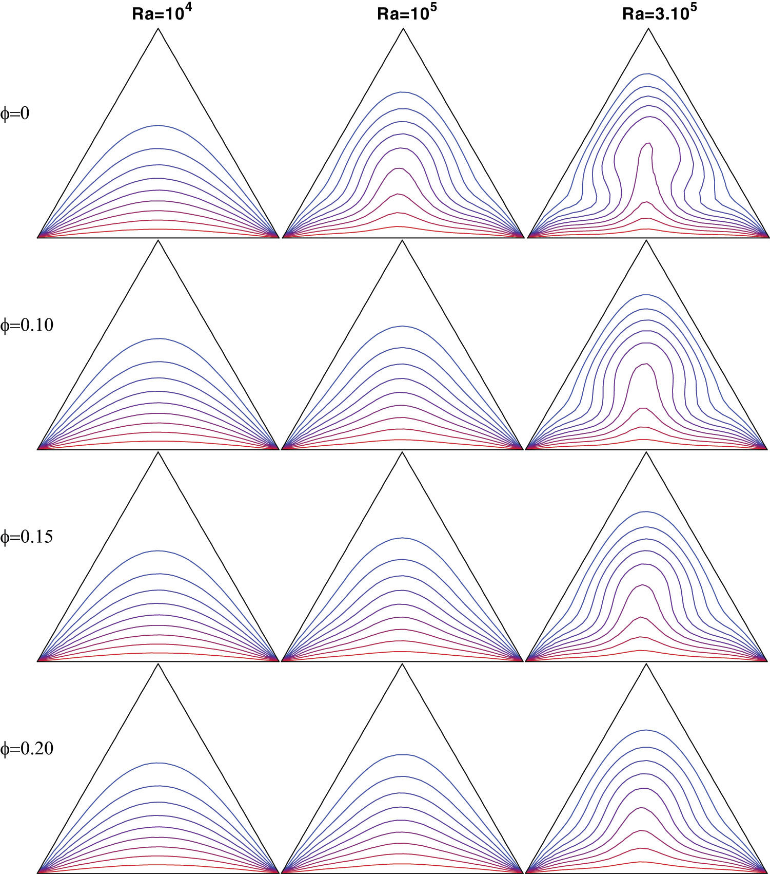
Figure 12: Isotherms of uniformly heated triangular cavity with a hot wall on the bottom, cold lateral walls, of Cu-water nanofluid, for volume fraction ϕ = 0.1, 0.15 and 0.2, and Rayleigh numbers of Ra = 104, 105 and 3.105
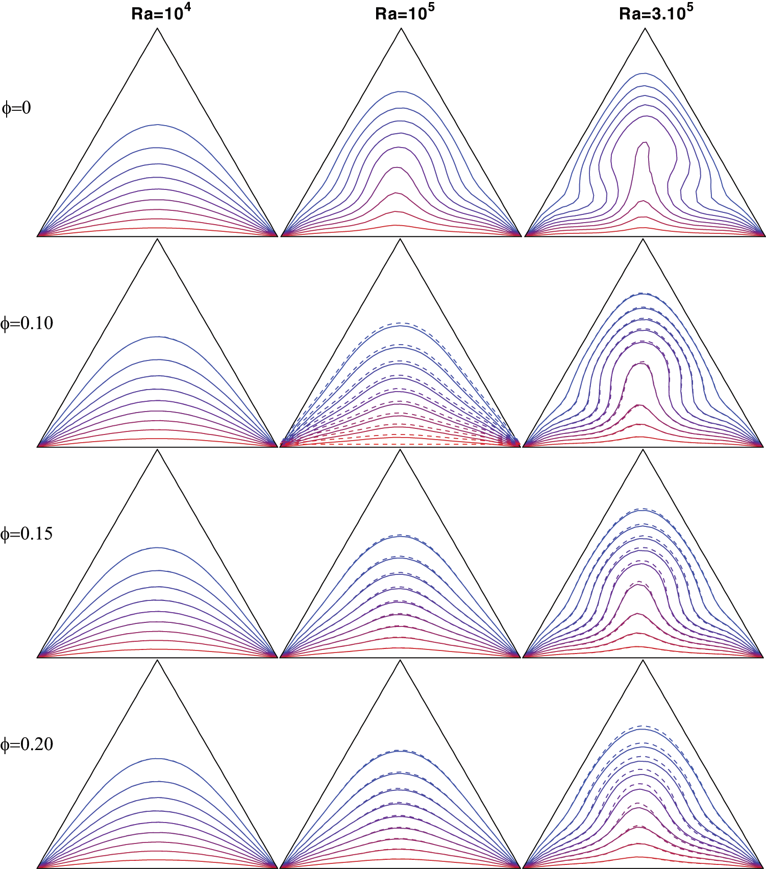
Figure 13: Isotherms of uniformly heated triangular cavity with a hot wall on the bottom, cold lateral walls, of Al2O3-water nanofluid (continued) and Cu-water (doted line), for volume fraction ϕ = 0.1, 0.15 and 0.2, and Rayleigh numbers of Ra = 104, 105 and 3.105
Figs. 12 and 13, for
In order to quantify the heat exchange within the cavity filled with Cu-water and
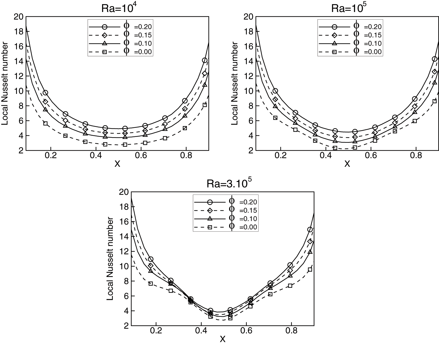
Figure 14: Local Nusselt number at the bottom wall for Cu-water nanofluid with the volume fractions ϕ = 0, 0.1, 0.15 and 0.2 at Rayleigh numbers 104, 105 and 3.105
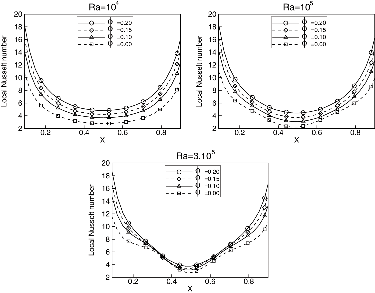
Figure 15: Local Nusselt number at the bottom wall for Al2O3-water nanofluid with the volume fractions ϕ = 0, 0.1, 0.15 and 0.2 at Rayleigh numbers 104, 105 and 3.105
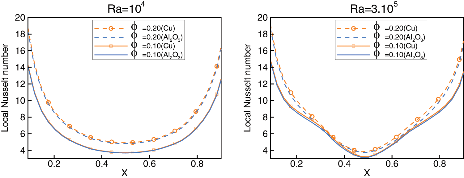
Figure 16: Comparison of local Nusselt number at the bottom wall for Cu-water and Al2O3-water nanofluid with the volume fractions ϕ = 0.10 and 0.2 at Rayleigh numbers 104 and 3.105
Fig. 17 shows the variation of the average Nusselt number as a function of the volume fraction for various values of the Rayleigh number. As can be seen, increasing the volume fraction results in higher average Nusselt number, this is due to the increased conductivity achieved by adding nanoparticles. Furthermore, these results confirm that Cu-water nanofluid is a better heat transfer fluid than
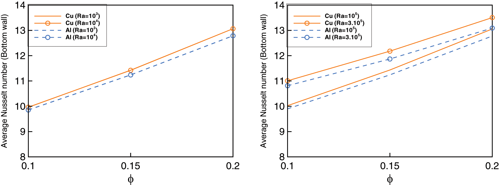
Figure 17: Variation of average Nusselt number with volume fractions of Cu and Al2O3 nanoparticles at different Rayleigh number
A two-dimensional numerical investigation of natural convection in enclose cavities was carried out in this study. Two geometries were used, namely those of a square and a triangular cavity. The laminar heat transfer equations of nanofluid were solved using the radial basis function method coupled with an artificial compressibility, which is classified as a meshless method. Cu-water and
• The implemented meshless method offers high flexibility in dealing with complex geometries due to the simplicity of the numerical evaluations of space derivative. This method provides a valuable and efficient way to analyze natural convection in nonrectangular geometries.
• To overcome the pressure velocity coupling problem that occurs in equation systems like the ones examined, the artificial compressibility model was implemented. The quality of the results was found to be of the same accuracy order as the other classical methods.
• Results clearly indicate that the addition of nanoparticles has produced a substantial enhancement of heat transfer as compared to that of the pure fluid. As mentioned above, convective transfer dominates conduction when Rayleigh numbers are increased. As a consequence, heat transfer from the hot walls to the cool walls is improved. This remains true for both of the cases investigated. Furthermore, we conclude that the heat transfer enhancement is not clear in low Rayleigh numbers or when the enclosures have geometric singularities, as was the case in our study, for the case of the triangular cavity.
Acknowledgement: The authors would like to acknowledge the financial support from King Faisal University, Saudi Arabia, Project No. AN000675.
Funding Statement: This work was supported through the Annual Funding Track by the Deanship of Scientific Research, Vice Presidency for Graduate Studies and Scientific Research, King Faisal University, Saudi Arabia [Project No. AN000675].
Conflicts of Interest: The authors declare that they have no conflicts of interest to report regarding the present study.
References
1. Yu, W., Choi, S. U. S. (2003). The role of interfacial layers in the enhanced thermal conductivity of nanofluids: A renovated Maxwell model. Journal of Nanopartical Research, 5, 167–171. DOI 10.1023/A:102443860380. [Google Scholar] [CrossRef]
2. Wasp, E. J., Kenny, J. P., Gandhi, R. L. (1979). Solid-liquid flow slurry pipeline transportation. Switzerland: Trans Tech Publications. [Google Scholar]
3. Souayeh, B., Ali Abro, K., Alfannakh, H., Al Nuwairan, M., Yasin, A. (2022). Application of Fourier sine transform to carbon nanotubes suspended in ethylene glycol for the enhancement of heat transfer. Energies, 15, 1200. DOI 10.3390/en15031200. [Google Scholar] [CrossRef]
4. Hamilton, R. L., Crosser, O. K. (1962). Thermal conductivity of heterogeneous two component systems. Industrial & Engineering Chemistry Fundamental, 1(3), 187–191. DOI 10.1021/i160003a005. [Google Scholar] [CrossRef]
5. Maxwell-Garnett, J. C. (1904). Colours in metal glasses and in metallic films. Philosophical Transactions of the Royal Society of London. Series A, Containing Papers of a Mathematical or Physical Character, 203, 385–420. DOI 10.1098/rsta.1904.0024. [Google Scholar] [CrossRef]
6. Al Nuwairan, M., Souayeh, B. (2021). Augmentation of heat transfer in a circular channel with inline and staggered baffles. Energies, 14(24), 8593. DOI 10.3390/en14248593. [Google Scholar] [CrossRef]
7. Choi, S. U. S. (1995). Enhancing thermal conductivity of fluids with nanoparticles. In: Siginer, D. A., Wang, H. P. (Eds.Developments and applications of non-newtonian flows, vol. 66, pp. 99--103. New York: The American Society of Mechanical Engineers. [Google Scholar]
8. Das, S., Choi, S., Wenhua, Y., Pradeep, T. (2007). Nonofluids: Science and technology. USA: Wiley. [Google Scholar]
9. Oztop, H. F., Abu-Nada, E. (2008). Numerical study of natural convection in partially heated rectangular enclosures filled with nanofluids. International Journal of Heat and Fluid Flow, 29(5), 1326–1336. DOI 10.1016/j.ijheatfluidflow.2008.04.009. [Google Scholar] [CrossRef]
10. Mahmoodi, M., Sebdani, S. M. (2012). Natural convection in a square cavity containing a nanofluid and an adiabatic square block at the center. Superlattices and Microstructures, 52(2), 261–275. DOI 10.1016/j.spmi.2012.05.007. [Google Scholar] [CrossRef]
11. Jasim, L. M., Hamzah, H., Canpolat, C., Sahin, B. (2021). Mixed convection flow of hybrid nanofluid through a vented enclosure with an inner rotating cylinder. International Communications in Heat and Mass Transfer, 121, 105086. DOI 10.1016/j.icheatmasstransfer.2020.105086. [Google Scholar] [CrossRef]
12. Bhowmick, D., Randive, P. R., Pati, S., Agrawal, H., Kumar, A. et al. (2020). Natural convection heat transfer and entropy generation from a heated cylinder of different geometry in an enclosure with non-uniform temperature distribution on the walls. Journal of Thermal Analysis and Calorimetry, 141(2), 839–857. DOI 10.1007/s10973-019-09054-2. [Google Scholar] [CrossRef]
13. Islam, T., Nur Alam, M., Asjad, M. I., Parveen, N., Chu, Y. (2021). Heatline visualization of MHD natural convection heat transfer of nanofluid in a prismatic enclosure. Scientific Reports, 11(1), 10972. DOI 10.1038/s41598-021-89814-z. [Google Scholar] [CrossRef]
14. Izadi, M., Mohebbi, R., Karimi, D., Sheremet, M. A. (2018). Numerical simulation of natural convection heat transfer inside a
15. Naseri Nia, S., Rabiei, F., Rashidi, M. M., Kwang, T. M. (2020). Lattice boltzmann simulation of natural convection heat transfer of a nanofluid in a L-shape enclosure with a baffle. Results in Physics, 19, 103413. DOI 10.1016/j.rinp.2020.103413. [Google Scholar] [CrossRef]
16. Pranowo, P., Wijayanta, A. (2018). The DMLPG method for numerical solution of Rayleigh-benard natural convection in porous medium. AIP Conference Proceedings, 1931, 030068. DOI 10.1063/1.5024127. [Google Scholar] [CrossRef]
17. Wijayanta, A., Pranowo, P. (2020). A localized meshless approach using radial basis functions for conjugate heat transfer problems in a heat exchanger. International Journal of Refrigeration, 110, 38–46. DOI 10.1016/j.ijrefrig.2019.10.025. [Google Scholar] [CrossRef]
18. Zhang, X., Zhang, P. (2015). Meshless modeling of natural convection problems in non-rectangular cavity using the variational multiscale element free galerkin method. Engineering Analysis with Boundary Elements, 61, 287–300. DOI 10.1016/j.enganabound.2015.08.005. [Google Scholar] [CrossRef]
19. Rostami, S., Toghraie, D., Shabani, B., Sina, N., Barnoon, P. (2021). Measurement of the thermal conductivity of MWCNT-CuO/water hybrid nanofluid using artificial neural networks (ANNs). Journal of Thermal Analysis and Calorimetry, 143, 1097–1105. DOI 10.1007/s10973-020-09458-5. [Google Scholar] [CrossRef]
20. Kavusi, H., Toghraie, D. (2017). A comprehensive study of the performance of a heat pipe by using of various nanofluids. Advanced Powder Technology, 28 (11), 3074–3084. DOI 10.1016/j.apt.2017.09.022. [Google Scholar] [CrossRef]
21. Rahmati, A. R., Akbari, O. A., Marzban, A., Toghaie, D., Karimi, R. et al. (2018). Simultaneous investigations the effects of non-newtonian nanofluid flow in different volume fractions of solid nanoparticles with slip and no-slip boundary conditions. Thermal Science and Engineering Progress, 5, 263–277. DOI 10.1016/j.tsep.2017.12.006. [Google Scholar] [CrossRef]
22. Ghasemi, B., Aminossadati, S. M. (2010). Periodic natural convection in a nanofluidfilled enclosure with oscillating heat flux. International Journal of Thermal Sciences, 49(1), 1–9. DOI 10.1016/j.ijthermalsci.2009.07.020. [Google Scholar] [CrossRef]
23. Maxwell, J. (1904). A treatise on electricity and magnetism, 2nd edition. Cambridge, UK: Oxford, University Press. [Google Scholar]
24. Brinkman, H. C. (1952). The viscosity of concentrated suspensions and solution. The Journal of Chemical Physics, 20, 571–581. DOI 10.1063/1.1700493. [Google Scholar] [CrossRef]
25. Kansa, E. J. (1990). Multiquadrics-A scattered data approximation scheme with applications to computational fluid-dynamics-I surface approximations and partial derivative estimates. Computers & Mathematics with Applications, 19(8–9), 127–145, DOI 10.1016/0898-1221(90)90270-T. [Google Scholar] [CrossRef]
26. Yao, G., Kolibal, J., Chen, C. S. (2011). A localized approach for the method of approximate particular solutions. Computers & Mathematics with Applications, 61(9), 2376–2387. DOI 10.1016/j.camwa.2011.02.007. [Google Scholar] [CrossRef]
27. Sarra, S. A. (2012). A local radial basis function method for advection-diffusion-reaction equations on complexly shaped domains. Applied Mathematics and Computation, 218(19), 9853–9865. DOI 10.1016/j.amc.2012.03.062. [Google Scholar] [CrossRef]
28. Tabbakh, Z., Seaid, M., Ellaia, R., Ouazar, D., Benkhaldoun, F. (2019). A local radial basis function projection method for incompressible flows in water eutrophication. Engineering Analysis with Boundary Elements, 106, 528–540. DOI 10.1016/j.enganabound.2019.06.004. [Google Scholar] [CrossRef]
29. Chorin, A. (1997). A numerical method for solving incompressible viscous flow problems. Journal of Computational Physics, 135(2), 118–125. DOI: 10.1006/jcph.1997.5716. [Google Scholar] [CrossRef]
30. Basak, T., Chamkha, A. J. (2012). Heatline analysis on natural convection for nanofluids confined within square cavities with various thermal boundary conditions. International Journal of Heat and Mass Transfer, 55(21–22), 5526–5543. DOI 10.1016/j.ijheatmasstransfer.2012.05.025. [Google Scholar] [CrossRef]
31. Pranowo, P., Wijayanta, A. (2021). Numerical solution strategy for natural convection problems in a triangular cavity using a direct meshless local petrov-galerkin method combined with an implicit artificial-compressibility model. Engineering Analysis with Boundary Elements, 126, 13–29. DOI 10.1016/j.enganabound.2021.02.006. [Google Scholar] [CrossRef]
Cite This Article
 Copyright © 2023 The Author(s). Published by Tech Science Press.
This work is licensed under a Creative Commons Attribution 4.0 International License , which permits unrestricted use, distribution, and reproduction in any medium, provided the original work is properly cited.
 Downloads
 Citation Tools