
 Submit a Paper
 Propose a Special lssue
 Open Access
ARTICLE
Unique Solution of Integral Equations via Intuitionistic Extended Fuzzy b-Metric-Like Spaces
1
Department of Mathematics, University of Management and Technology, Lahore, 54770, Pakistan
2
Department of Math & Stats, International Islamic University Islamabad, Islamabad, 44000, Pakistan
3
Abdus Salam School of Mathematical Sciences, Government College University, Lahore, 54600, Pakistan
4
Office of Research, Innovation and Commercialization, University of Management and Technology, Lahore, 54770, Pakistan
5
Department of Mathematics and Sciences, Prince Sultan University, Riyadh, 11586, Saudi Arabia
6
Department of Medical Research, China Medical University, Taichung, 40402, Taiwan
7
Department of Mathematical Sciences, Faculty of Sciences, Princess Nourah Bint Abdulrahman University,
Riyadh, 11671, Saudi Arabia
* Corresponding Author: Thabet Abdeljawad. Email:
Computer Modeling in Engineering & Sciences 2023, 135(1), 109-131. https://doi.org/10.32604/cmes.2022.021031
Received 24 December 2021; Accepted 25 May 2022; Issue published 29 September 2022
 View Full Text
 Download PDF
Abstract
In this manuscript, our goal is to introduce the notion of intuitionistic extended fuzzy b-metric-like spaces. We establish some fixed point theorems in this setting. Also, we plot some graphs of an example of obtained result for better understanding. We use the concepts of continuous triangular norms and continuous triangular conorms in an intuitionistic fuzzy metric-like space. Triangular norms are used to generalize with the probability distribution of triangle inequality in metric space conditions. Triangular conorms are known as dual operations of triangular norms. The obtained results boost the approaches of existing ones in the literature and are supported by some examples and applications.Keywords
After being given the notion of fuzzy sets (FSs) by Zadeh [1], many researchers provided many generalizations. Schweizer et al. [2] introduced the notion of continuous t-norms. In this continuation, Kramosil et al. [3] introduced the approach of fuzzy metric spaces, while George et al. [4] introduced the concept of fuzzy metric spaces. Garbiec [5] gave the fuzzy interpretation of the Banach contraction principle in fuzzy metric spaces. Dey et al. [6] established an extension of Banach fixed point theorem in fuzzy metric space. Nadaban [7] introduced the notion of fuzzy b-metric spaces. Gregory et al. [8] proved various fixed point theorems in fuzzy metric spaces. Bashir et al. [9] established several fixed point results of a generalized reversed F-contraction mapping and its application.
Recently, Harandi [10] initiated the concept of metric-like spaces, which generalized the notion of metric spaces in a nice way. Alghamdi et al. [11] used the concept of metric-like spaces and introduced the notion of b-metric-like spaces. In this sequel, Shukla et al. [12] generalized the concept of metric-like spaces and introduced fuzzy metric-like spaces and Javed et al. [13] introduced the concept of fuzzy b-metric-like spaces and prove some fixed point results.
Mehmood et al. [14] presented the notion of fuzzy extended b-metric spaces (FEBMSs) by replacing the coefficient
In this manuscript, we aim to introduce the concept of intuitionistic extended fuzzy b-metric-like space (IEFBMLS). In which, we generalize the concept of IFBMS by replacing the coefficient
Main objectives of this manuscript are:
(a) To introduce the notion of intuitionistic extended fuzzy b-metric-like space.
(b) To enhance the literature of intuitionistic fuzzy fixed point theory.
(c) To plot some graphical structure of obtained result.
(d) To prove the existence and uniqueness of established results via integral equations.
(e) To provide an application dynamic market equilibrium.
The following definitions are helpful in the sequel.
Definition 2.1 [15] A binary operation
1.
2.
3.
4.
5. If
Definition 2.2 [15] A binary operation
1.
2.
3.
4.
5. If
Definition 2.3 [10] A mapping
a.
b.
c.
for all
Definition 2.4 [12] Take
(F1)
(F2)
(F3)
(F4)
(F5)
Definition 2.5 [14] A 4-tuple
Δ1)
Δ2)
Δ3)
Δ4)
Δ5)
Definition 2.6 [31] Take
(I)
(II)
(III)
(IV)
(V)
(VI)
(VII)
(VIII)
(IX)
(X)
(XI)
In this section, we introduce the notion of an IEFBMLS and prove some related FP results.
Definition 3.1 Let
(i)
(ii)
(iii)
(iv)
(v)
(vi)
(vii)
(viii)
(ix)
(x)
(xi)
Remark 3.2 In the above definition, the self distance in condition (iii) may not be equal to 1 and in condition (viii) the self distance may not be equal to 0. In triangular inequalities, we use
Example 3.3 Let
for all
Then
Example 3.4 Let
and
Then
Remark 3.5 Above example also satisfied for CTN
Example 3.6 Let
and
Then
Proposition 3.7 Let
Then
Remark 3.8 The above proposition also satisfied for CTN
Proposition 3.9 Let
Then
Example 3.10 Let
for all
Then
Remark 3.11 In the above all examples self distance may not be equal to 1 and 0. In particular, assume an example 3.9, take
Remark 3.12 In the above Examples 3.3, 3.4, 3.6, 3.7, 3.10 and Proposition 3.9, it is easy to see that self-distance is not equal to 1 as in condition (iii) and the self-distance is not equal to 0 as in condition (viii) in Definition 3.1. So, the Examples 3.3, 3.4, 3.6, 3.7, 3.10 and Proposition 3.9 are becomes IEFBMLSs but not becomes IFBMSs.
Definition 3.13 Let
(a) A sequence
(b) A sequence
(c) An IEFBMS is named to be complete iff each GCS is convergent, i.e.,
Now, we consider intuitionistic extended fuzzy like contractions.
Theorem 3.14 Let
for all
for all
where
Proof: Let
and
We obtain
for any
and
Using (3)
and
We obtain for all
That is,
Now, using
and
This implies that
and
By using
Example 3.15 Let
and
with CTN
Then clearly
Let
and
Observe that all the conditions of Theorem 3.14 are satisfied and 0 is a unique fixed point, i.e.,
Now, we use the Example 3.15 to show the graphical view of contraction mapping and a unique fixed point. Below, in Fig. 1, we show the graphical view of Mφ (f ϑ, f δ, kT) = Mφ (ϑ, δ, T ). Table 1 shows the values of Mφ (f ϑ, f δ, kT) and Table 2 shows the values of Mφ (ϑ, δ, T). In Fig. 2, we show the graphical view of Nφ (f ϑ, f δ, kT) = Nφ (ϑ, δ, T). Table 3 shows the values of Nφ (f ϑ, f δ, kT ) and Table 4 shows the values of Nφ (ϑ, δ, T). In Fig. 3, we show the view of unique fixed point.
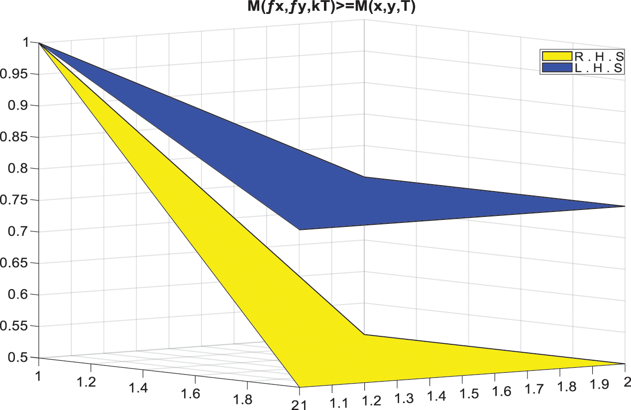
Figure 1: Variation of L.H.S. =


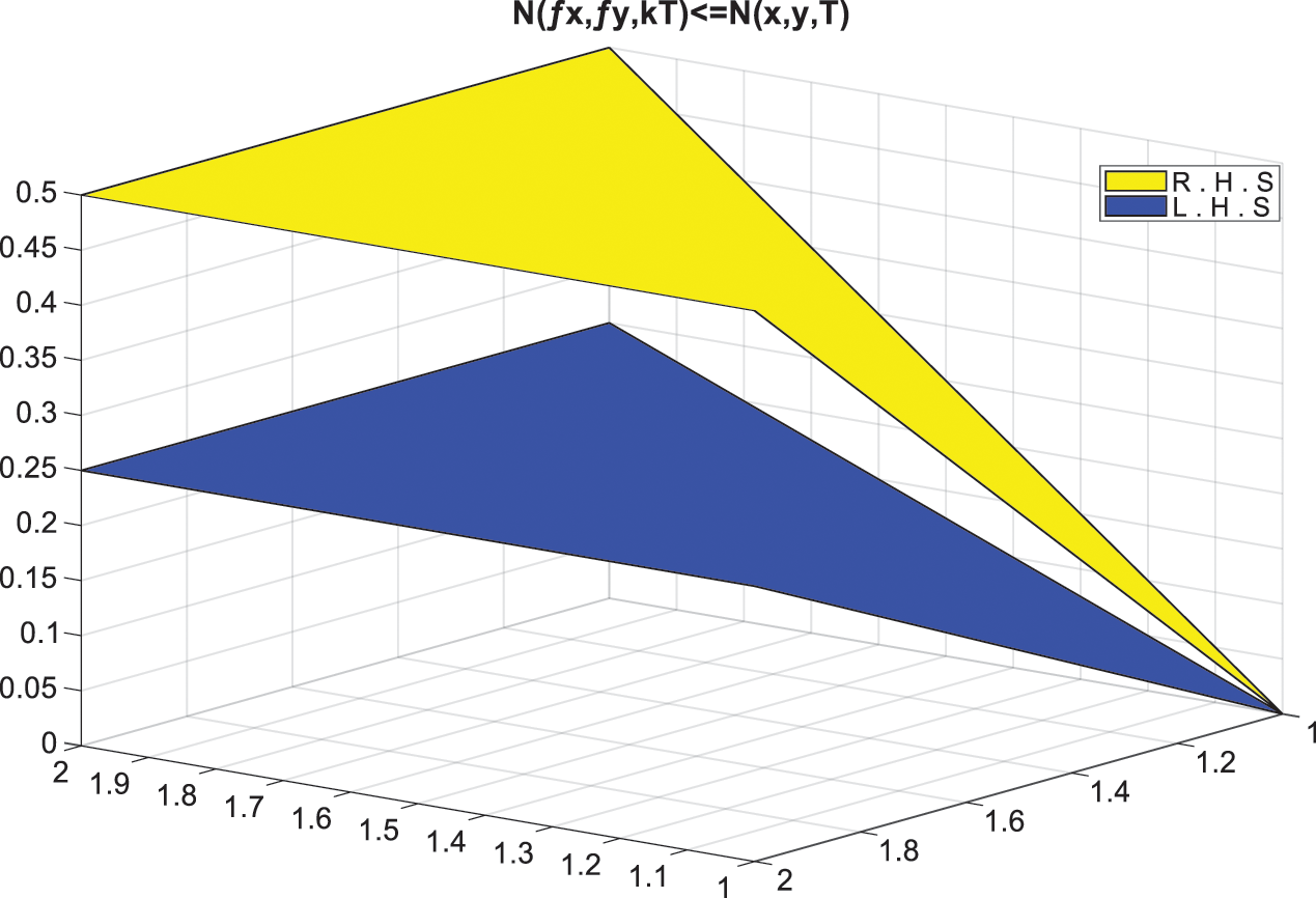
Figure 2: Variation of L.H.S. =


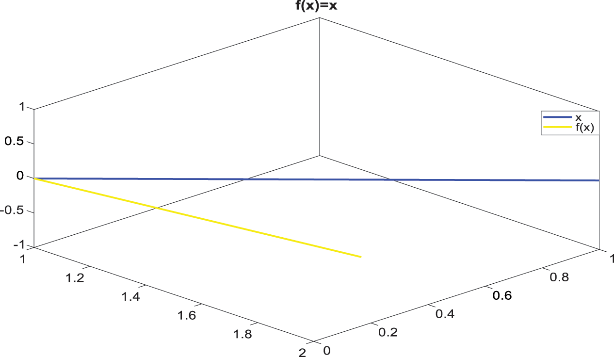
Figure 3: Graph of
Definition 3.16 Let
and
for all
Now, we prove the following theorem related to above contraction mapping.
Theorem 3.17 Let
for all
Proof: Let
That is
Continuing in this way, we get
We obtain
and
for all
and
Using (3),
and
Consequently, for all
i.e.,
Now, we investigate that
That is,
It implies that
and
This yields that
which is a contradiction. Also,
Again, it is a contradiction. Therefore, we must have
Example 3.18 Let
Also take
with
Then we have four cases:
1. If
2. If
3. If
4. If
In all
are satisfied for
Satisfied for
Observe that all circumstances of Theorems 3.14 and 3.17 are fulfilled, and 0 is a unique FP of f.
Example 3.19 Let
for all
Then,
are satisfied for
and
satisfied for
Observe that all circumstances of Theorems 3.14 and 3.17 are fulfilled, and 0 is a unique FP of f.
4 Application to Fuzzy Fredholm Integral Equations
Let
Now, we let the fuzzy integral equation
where
and
for all
Then
Assume that
Proof: Define
Scrutinize that survival of an FP of the operator f is come to the survival of solution of the fuzzy integral equation.
Now for all
Therefore, all the conditions of Theorem 3.11 are fulfilled. Hence operator f has a unique FP. This implies that fuzzy integral Eq. (9) has a unique solution.
Corollary 3.1 Let
Suppose the below conditions meet:
I.
II.
Then integral Eq. (9) has a solution.
We can prove easily by follow the above proof.
5 Application to Dynamic Market Equilibrium
In real business cycle models, economy is always in its long run equilibrium but in Keynesian business cycle theory the economy could be above or below the long-term potential, full employment GDP. While the real business cycle model seeks to overcome the distinction between the long run growth model and the real business cycle. Now we show how our established result can be used to find the unique solution to an integral equation in dynamic market equilibrium economics.
Let us denote the supply
since
Letting
Dividing through by
where
where
We will show the existence of a solution to the integral equation
Let
and
for all
It is easy to show that
Theorem 4.1 Consider Eq. (11) and suppose that
(i)
(ii) There exist a continuous function
(iii)
Then, the integral Eq. (11) has a unique solution.
Proof: For
and
Thus
Herein, we introduced the notion of intuitionistic extended fuzzy b-metric-like spaces and some new types of fixed point theorems in this new setting. Moreover, we provided non-trivial examples and plotted some graphs to demonstrate the viability of the proposed methods. We provided an application of the obtained results in a dynamic equilibrium market. We have supplemented this work with applications demonstrating how the built method outperforms those found in the literature. Since our structure is more general than the class of fuzzy b-metric like space and intuitionistic fuzzy b-metric space, our results and notions expand and generalize several previously published results. This work can easily extend to the structure of neutrosophic extended b-metric-like spaces, controlled intuitionistic fuzzy b-metric-like spaces, and many other structures.
Acknowledgement: The authors are grateful to their universities for their support.
Author’s Contributions: All authors contributed equally in writing this article. All authors read and approved the final manuscript.
Availability of Data and Materials: Data sharing is not applicable to this article as no data sets were generated or analyzed during the current study.
Funding Statement: Princess Nourah bint Abdulrahman University Researchers Supporting Project No. (PNURSP2022R14), Princess Nourah bint Abdulrahman University, Riyadh, Saudi Arabia.
Conflicts of Interest: The authors declare that they have no conflicts of interest to report regarding the present study.
References
1. Zadeh, L. A. (1965). Fuzzy sets. Information and Control, 8(3), 338–353. DOI 10.1016/S0019-9958(65)90241-X. [Google Scholar] [CrossRef]
2. Schweizer, B., Sklar, A. (1960). Statistical metric spaces. Pacific Journal of Mathematics, 10(1), 314–334. DOI 10.2140/pjm. [Google Scholar] [CrossRef]
3. Kramosil, I., Michlek, J. (1975). Fuzzy metric and statistical metric spaces. Kybernetika, 11(5), 336–344. [Google Scholar]
4. George, A., Veeramani, P. (1994). On some results in fuzzy metric spaces. Fuzzy Sets and Systems, 64(3), 395–399. DOI 10.1016/0165-0114(94)90162-7. [Google Scholar] [CrossRef]
5. Grabiec, M. (1988). Fixed points in fuzzy metric spaces. Fuzzy Sets and Systems, 27(3), 385–389. DOI 10.1016/0165-0114(88)90064-4. [Google Scholar] [CrossRef]
6. Dey, D., Saha, M. (2014). An extension of banach fixed point theorem in fuzzy metric space. Boletim da Sociedade Paranaense de Matematica, 32(1), 299–304. DOI 10.5269/bspm.v32i1.17260. [Google Scholar] [CrossRef]
7. Nadaban, N. (2016). Fuzzy b-metric spaces. International Journal of Computers Communications and Control, 11(2), 273–281. DOI 10.15837/ijccc.2016.2.2443. [Google Scholar] [CrossRef]
8. Gregory, V., Sapena, A. (2002). On fixed point theorems in fuzzy metric spaces. Fuzzy set and Systems, 125(2), 245–253. DOI 10.1016/S0165-0114(00)00088-9. [Google Scholar] [CrossRef]
9. Bashir, S., Saleem, N., Husnine, S. M. (2021). Fixed point results of a generalized reversed F-contraction mapping and its application. Aims Mathematics, 6(8), 8728–8741. DOI 10.3934/math.2021507. [Google Scholar] [CrossRef]
10. Harandi, A. (2012). Metric-like spaces, partial metric spaces and fixed points. Fixed Point Theory and Applications, 2012(1), 1–10. [Google Scholar]
11. Alghamdi, M. A., Hussain, N., Salimi, P. (2013). Fixed point and coupled fixed point theorems on b-metric-like spaces. Journal of Inequalities and Applications, 2013(1), 1–25. DOI 10.1186/1029-242X-2013-402. [Google Scholar] [CrossRef]
12. Shukla, S., Abbas, M. (2014). Fixed point results in fuzzy metric-like spaces. Iranian Journal of Fuzzy Systems, 11(5), 81–92. [Google Scholar]
13. Javed, K., Uddin, F., Aydi, H., Arshad, M., Ishtiaq, U. et al. (2021). On fuzzy b-metric-like spaces. Journal of Function Spaces, 2021, 1–10. DOI 10.1155/2021/6615976. [Google Scholar] [CrossRef]
14. Mehmood, F., Ali, R., Ionescu, C., Kamran, T. (2017). Extended fuzzy b-metric spaces. Journal of Mathematical Analysis, 6(8), 124–131. [Google Scholar]
15. Park, J. H. (2004). Intuitionistic fuzzy metric spaces. chaos. Solitons and Fractals, 22(5), 1039–1046. DOI 10.1016/j.chaos.2004.02.051. [Google Scholar] [CrossRef]
16. Rafi, M., Noorani, M. S. M. (2006). Fixed theorems on intuitionistic fuzzy metric space. Iranian Journal of Fuzzy Systems, 3(1), 23–29. [Google Scholar]
17. Alaca, C., Turkoglu, D., Yildiz, C. (2006). Fixed points in intuitionistic fuzzy metric spaces. Chaos, Solitons and Fractals, 29(5), 1073–1078. DOI 10.1016/j.chaos.2005.08.066. [Google Scholar] [CrossRef]
18. Mohamad, A. (2007). Fixed-point theorems in intuitionistic fuzzy metric spaces. Chaos, Solitons and Fractals, 34(5), 1689–1695. DOI 10.1016/j.chaos.2006.05.024. [Google Scholar] [CrossRef]
19. Saleem, N., Iqbal, I., Iqbal, B., Radenovic, S. (2020). Coincidence and fixed points of multivalued F-contractions in generalized metric space with application. Journal of Fixed Point Theory and Applications, 22(4), 1–24. DOI 10.1007/s11784-020-00815-3. [Google Scholar] [CrossRef]
20. Saleem, N., Ali, B., Raza, Z., Abbas, M. (2019). Fixed points of suzuki-type generalized multivalued (f, θ, L) almost contractions with applications. Filomat, 33(2), 499–518. DOI 10.2298/FIL1902499S. [Google Scholar] [CrossRef]
21. Saleem, N., Abbas, M., de la sen, M. (2019). Optimal approximate solution of coincidence points equations in fuzzy metric spaces. Mathematics, 7(4), 1–13. DOI 10.3390/math7040327. [Google Scholar] [CrossRef]
22. Saleem, N., Abbas, M., Raza, Z. (2017). Fixed fuzzy point results of generalized suzuki type F-contraction mappings in ordered metric spaces. Georgian Journal of Mathematics, 24(4), 1–14. [Google Scholar]
23. de la sen, M., Abbas, M., Saleem, N. (2017). On optimal fuzzy best proximity coincidence points of proximal contractions involving cyclic mappings in non-archimedean fuzzy metric spaces. Mathematics, 5(2), 1–20. [Google Scholar]
24. Saleem, N., Abbas, M., Raza, Z. (2016). Optimal coincidence best approximation solution in non-archimedean fuzzy metric spaces. Iranian Journal of Fuzzy Systems, 13(3), 113–124. [Google Scholar]
25. Abbas, M., Saleem, N., de la sen, M. (2016). Optimal coincidence point results in partially ordered non-archimedean fuzzy metric spaces. Fixed Point Theory and Applications, 2016(1), 1–18. DOI 10.1186/1687-1812-2012-1. [Google Scholar] [CrossRef]
26. Saleem, N., Ali, B., Abbas, M., Raza, Z. (2015). Fixed points of suzuki type generalized multivalued mappings in fuzzy metric spaces with applications. Fixed Point Theory and Applications, 2015(1), 1–18. DOI 10.1186/s13663-015-0284-7. [Google Scholar] [CrossRef]
27. Shukla, S., Gopal, D., Roldán-López-deHierro, A. F. (2016). Some fixed point theorems in 1-M-complete fuzzy metric-like spaces. International Journal of General Systems, 45(8), 815–829. DOI 10.1080/03081079.2016.1153084. [Google Scholar] [CrossRef]
28. Abbas, M., Lael, F., Saleem, N. (2020). Fuzzy b-metric spaces: Fixed point results for contraction correspondences and their application. Axioms, 9(2), 1–12. DOI 10.3390/axioms9020036. [Google Scholar] [CrossRef]
29. Sintunavarat, W., Kumam, P. (2012). Fixed theorems for a generalized intuitionistic fuzzy contraction in intuitionistic fuzzy metric spaces. Thai Journal of Mathematics, 10(1), 123–135. [Google Scholar]
30. Saadati, R., Park, J. H. (2006). On the intuitionistic fuzzy topological spaces. Chaos, Solitons and Fractals, 27(2), 331–344. DOI 10.1016/j.chaos.2005.03.019. [Google Scholar] [CrossRef]
31. Konwar, K. (2020). Extension of fixed results in intuitionistic fuzzy b-metric spaces. Journal of Intelligent & Fuzzy Systems, 39(5), 7831–7841. DOI 10.3233/JIFS-201233. [Google Scholar] [CrossRef]
32. Mahmood, T., Ali, W., Ali, Z., Chinram, R. (2021). Power aggregation operators and similarity measures based on improved intuitionistic hesitant fuzzy sets and their applications to multiple attribute decision making. Computer Modeling in Engineering & Sciences, 126(3), 1165–1187. DOI 10.32604/cmes.2021.014393. [Google Scholar] [CrossRef]
Cite This Article
 Copyright © 2023 The Author(s). Published by Tech Science Press.
This work is licensed under a Creative Commons Attribution 4.0 International License , which permits unrestricted use, distribution, and reproduction in any medium, provided the original work is properly cited.
 Downloads
 Citation Tools