Efficient Origin-Destination Estimation Using Microscopic Traffic Simulation with Restricted Rerouting

1  Introduction

Traffic simulation is used to solve various traffic problems and inform associated policies such as handling congestion or accidents, controlling CO2 emissions, and guaranteeing mobility in aging societies. Many simulation models have been developed, and they can be roughly divided into macroscopic, mesoscopic, and microscopic models. The macroscopic models approximate aggregated vehicles as a continuous flow on links, where some form of traffic assignment models assign each link demand. The microscopic models treat each vehicle as a particle, making it possible to distinguish individual vehicles and thus to describe vehicles’ precise behaviors. In contrast to macroscopic models, each vehicle has its own route along which it travels in some microscopic models. The mesoscopic models are just the middle of the macroscopic models and the microscopic models. While each vehicle is identified like microscopic models, the behavior is expressed in a macroscopic manner.

The simulation model and input data must be reliable and realistic to reproduce a realistic traffic situation in a simulator. And in most cases, a single simulator is used for parametric studies by changing some parameters sets. In this research, the authors focus on the reliability of traffic demand as the input data given to the simulator.

We can easily obtain road structure information (e.g., intersection configuration) and observable and controllable information (e.g., traffic light patterns) in the real world. However, traffic demand data, which directly affect link traffic volume, congestion, and service levels, are more difficult to obtain because of their unobservability and significant uncertainties.

Origin-destination (OD) matrices describe traffic demand. An OD matrix consists of traffic demand (traffic volume) for each OD pair, i.e., a pair of an origin and a destination point. Rows and columns of an OD matrix denote origins and destinations, respectively. For example, the (r,c) element in an OD matrix represents the number of vehicles per unit time that flow into the road network at origin point Or and flow out at destination Dc. The unit of traffic demand is often given in vehicles per hour, veh/h in short.

The authors regard OD estimation as a bi-level programming problem and target OD estimation problem for microscopic traffic simulation, especially. In this situation, the same traffic model should be employed in both lower and upper problems to make the input and the output for those problems consistent.

It is concerned that the computational time increases due to the dynamic rerouting in each simulation trial and the increased number of trial iterations when using such a method. Dynamic rerouting is a route search operation required when a vehicle driver faces a high-cost link to pass (e.g., a congested link) during driving along the route acquired by the initial search. Thus, dynamic rerouting is reasonable because it corresponds to each driver’s detour behavior. By introducing dynamic rerouting, vehicles detour to avoid congestion, and consequently, congestions are relaxed. However, each route search operation, including dynamic rerouting, is computationally expensive. In addition, each vehicle driver should know the traffic situation of the route candidates at a specific time point to reroute dynamically. It is concerned to be an unrealistic assumption beyond the vehicle drivers’ capability. The authors propose a way to suppress the number of dynamic rerouting in OD estimation and deal with the problems resulting from this restriction.

2  Literature Review

Three general approaches are available for OD estimation: statistical approaches, traffic volume optimization approaches with demand assignment, and traffic volume optimization approaches with microscopic simulators. In the statistical approaches, the OD matrices are generated by aggregating survey data, which can come from personal interviews. A typical example is the four-step model [1], widely utilized for long-term demand prediction since the 1950s.

The traffic volume optimization approaches with demand assignment optimize link traffic volume, i.e., match the volume in the simulation to that in the real world by changing the solution candidates for the OD matrices. The assignment of traffic demand for each link is determined under the assumption of logit-based decision rules and user equilibrium (UE) theory. Most such methods handle traffic flow with stochastic turbulence based on minimum entropy [2–4], maximum likelihood [5,6], or generalized least squares optimization [7]. For further details, see [8].

The statistical and traffic volume optimization approaches with demand assignment handle wide-ranging and aggregated traffic flows. Therefore, these methods are often applied in macroscopic simulators because of the characteristics of aggregated flow.

Microscopic simulators are also widely used. These simulators seek to capture more detailed traffic phenomena. A multi-agent system (MAS) is commonly used to implement such models. The MAS captures each agent’s autonomous recognition, decision-making, and action. When applied to traffic simulation, the MAS regards each driver or each vehicle as an agent. Entire phenomena such as congestion emerge from the interactions among the drivers. Since this type of modeling directly incorporates the individual behavior of actual drivers, the MAS is suitable for simulating traffic phenomena in the real world at a fine-scale resolution. The MAS employs route search algorithms (e.g., Dijkstra’s algorithm [9] or the A* algorithm [10]) where each vehicle agent constructs its preferable route considering heterogeneity and the dynamic changes in the traffic situation. In recent years, many multi-agent-based microscopic simulators have been applied, including VISSIM [11], Aimsun [12], SUMO [13], ADVENTURE_Mates [14,15] and MATSim [16].

Microscopic traffic simulations based on a MAS require OD matrices as traffic demand input data. In one traffic volume optimization approach using a MAS-based simulator for OD estimation, Nguyen et al. applied the DFROUTER tool to SUMO. This tool reconstructs vehicle routes based on detector measurements [17]. Shafiei et al. proposed a gradient-based method using a linear approximation for the demand-link traffic volume relation [18]. The simultaneous perturbation stochastic approximation model (SPSA) [19] has also been proposed for OD estimation in microscopic simulations, including MAS-based models. SPSA is one of the gradient-based models that minimize the absolute error in the simulated link traffic volume (i.e., the difference between the simulated volume and the observed volume). Unlike the original gradient-based model, the gradient is calculated stochastically in the SPSA so that it is tolerant to noise. Yang et al. employed the SPSA for OD matrix optimization with VISSIM [20]. Here, VISSIM is not only the simulation model itself; it is also a part of the OD matrix estimation model. Thus, the estimated OD matrices provide consistent input data for the VISSIM simulator. Djukic et al. applied the SPSA method to Aimsun, where both microscopic and macroscopic models were employed [21]. There are also other OD estimation studies using SPSA, e.g. [22,23].

Omrani and Lina proposed a genetic-algorithm (GA)-based approach for OD estimation [24]. They used a genetic algorithm to calibrate parameters affecting route choice behavior in the simulation. Marzano et al. applied a Kalman-filter for OD estimation [25]. Yousefikia et al. proposed the TflowFuzzy method, which is based on fuzzy set theory [26]. These methods use bi-level programming; the update process for the OD matrix solution candidates and the simulation process are divided and conducted alternately. Theoretically, we can apply these methods based on bi-level programming to congested traffic situations in the real world [8].

Because drivers’ dynamic rerouting behaviors avoid the uneven distribution of vehicles in a network, bi-level-programming-based approaches employing MAS-based microscopic simulators within the model tend to work well. However, these approaches can involve significantly higher computational costs for the dynamic rerouting process, as each driver search for the shortest path frequently. For example, SPSA requires two simulation runs to determine the gradient [27]. Thus, using a fine-modeled simulator for a large-scale network can be computationally quite expensive.

Nowadays, several OD estimation methods using advanced deep learning models have been proposed [28,29]. For example, Tang et al. proposed the method using the 3D convolution-based deep neural network (NN), Res3D, to estimate the OD matrices in Shanghai. Koca et al. proposed the graph NN to estimate the OD matrices in New York. These researches aim to estimate OD matrices by inputting numerous vehicle coordinate data into learned NNs. However, there are difficulties in employing advanced deep learning models to estimate OD matrices used in microscopic traffic simulations. For example, Koca et al. [29] reported that the coefficient of determination in link traffic volume is less than or equal to 0.3 in the cross-validation in which data obtained in an area were input into the model learned in another area. In other words, the versatility of NN-based methods is not sufficient. Consequently, as with other methods that do not incorporate microscopic simulators, the OD matrices estimated by the NN-based methods may be inconsistent with the simulator that intends to use them.

3  Methodology

3.1 Aims

As mentioned in the previous section, this research aims to solve the OD estimation problem using a MAS-based simulator with restricted dynamic rerouting functions. Here, the simulator allows a vehicle agent to reroute only after finding itself in an unintended route, which can occur when a lane is blocked due to congestion. By restricting dynamic rerouting, it is expected that the computational cost will be reduced and that vehicle drivers’ routing behavior will be more feasible.

However, employing such a restricted MAS-based simulator faces several challenges in the OD estimation process. If high traffic demand is assigned to a low-throughput route in a certain iteration step, congestion may occur at intersections. This is a natural characteristic in real situations, and if full dynamic rerouting is allowed, the demand is adequately distributed to mitigate the congestion. But, when the restricted dynamic rerouting proposed in this paper is employed, a kind of positive feedback occurs so that heavier congestion arises at successive iteration steps. Once congestion incurs stuck of vehicles upstream of the observation point, the link traffic volume, i.e., the number of vehicles that passed the link, is under-measured compared to the link traffic demand, i.e., the number of vehicles that intend to pass the link. In order to resolve this shortage of link traffic volume, more vehicles are assigned to pass the link, regardless of whether it is the congested link or not. Consequently, the congestion becomes even heavier, and the traffic volume is further reduced unexpectedly. This traffic congestion generated by the restricted simulator functions is hereafter referred to as “fictitious congestion”.

To resolve the fictitious congestion problem, the authors introduce upper-bound constraints for link demand reflecting a congested state in the OD estimation process. It is handled outside the simulator used in the OD estimation process. As a result, the proposed method is applicable to simulators even when dynamic rerouting is fully available.

3.2 Overview

The authors aim to solve the following two problems: (1) calculation cost for bi-level-programming-based OD estimation and (2) fictitious congestion when employing the simulator with restricted dynamic rerouting. Especially, the OD estimation method is not established in context of restricted dynamic rerouting. In this paper, the OD estimation problem is solved based on a framework that deals with OD traffic volume assignment to links by alternately using simulation and optimization of the solution candidate of the OD matrix via a numerical solver. Within this framework, a MAS-based simulator with restricted dynamic rerouting is employed. By using this simplified framework, the computational cost can be substantially reduced. To demonstrate the practical performance of the proposed method, three cases were tested: a low-demand case, a high-demand case with link demand constraints, and a high-demand case without link demand constraints.

A flowchart of the proposed OD estimation method is shown in Fig. 1. This is based on the authors’ previously proposed OD estimation method that embeds a MAS-based simulator [30,31].

Figure 1: Flowchart of proposed OD estimation method

Here, x denotes the OD matrix in vector form. The dimension of x is N, the number of OD pairs. Q¯ and Q^ denote the observed and simulated link traffic volumes, respectively. The observed link traffic volumes are given from the beginning; the simulated link traffic volumes are obtained from simulation results with the OD matrix x. (k) denotes the iteration number. T denotes transposition. r denotes the residual of the observed and simulated link traffic volumes; that is, r=Q¯−Q^. The dimensions of r, Q¯ and Q^ are all M. In general, N is larger than M. j denotes the index of OD pairs. xu denotes the common upper bound of each OD traffic volume. This value is a constant regardless of the importance of the OD pair such as trunk or branch ones.

The estimation process starts with an initial OD matrix in vector form, x(k)=x(0). In this form, each element of the vector denotes an OD traffic volume. Next, a simulation is conducted with the OD matrix x(k) to obtain the simulated link traffic volume in vector form Q^(k) and assignment matrix A(k), which is explained in Subsection 3.3. Convergence is then examined. If the root mean square error (RMSE), as defined in Eq. (1), in the k-th iteration step is smaller than a threshold value ε or the iteration number reaches the maximum number of iterations kmax, the solution is judged to have converged. ε is often determined considering the total traffic demand or variant of that.

RMSE=‖r‖2M.(1)

If the solution does not converge, a new OD matrix candidate is calculated by solving a quadratic programming (QP) problem. When the QP is solved, some constraints corresponding to the congestion situation are considered. The Fig. 1 indicates this operation as Congestion detection and Sign inversion. The detail is described in Section 3.3. These operations are iterated until a solution candidate converges. The flow of alternately conducting the simulation and solving the QP problem corresponds to a bi-level programming problem. To avoid an overly long computational time, a QP solver is used iteratively instead of the SPSA. Details of the formulation and variables are given in Subsection 3.3.

To simplify the OD estimation problem, the authors assume that the traffic situation is nearly steady during a one-hour simulation. This assumption is based on the fact that link traffic volume is aggregated every hour in many data sources. Importantly, this OD estimation is performed offline, i.e., all the link traffic volumes are determined before the estimation starts. By focusing on a particular one-hour period to be estimated, the model can be considered static. There is no problem discussing the function of dynamic rerouting under the assumption of static conditions because the MAS itself shows a dynamic process. The behavior of an agent means that the environment is dynamically changing for other agents.

The fictitious congestion appears in a simulation during the OD estimation process. In reality, even if congestion occurs, it will be resolved over time due to drivers’ dynamic rerouting behavior. However, under the assumption of the static OD matrix, with the difficulty of detouring as explained in Section 2, the congestion will not be resolved since link demand is constant during the targeted hour, even if the link is congested. In such a situation, congestions must be avoided, i.e., there should be no assignment of higher demand than the link traffic capacity. Here, the authors define fictitious congestion more concretely: It is the emergence of a vehicle queue that continuously exceeds a certain length in a simulation during the OD estimation. Then, whether or not fictitious congestion appears can be distinguished in terms of the simulation results. The authors seek to reduce the fictitious congestion by modifying the OD matrix rather than invoking dynamic rerouting in the simulation.

3.3 Formulation

In the proposed method, the residual between the observed and simulated link traffic volumes is minimized subject to constraints on OD traffic volume, as a kind of QP problem. The optimization problem with the objective function and its constraints is

minimizef(x),s.t.0≤xj≤xu∀j,(2)

where

f(x)=‖r‖2=‖Q¯−Q^‖2.(3)

To solve Eq. (2), the authors assume a relation between the OD matrix and link traffic volume as

Q^=Ax.(4)

This assumption means that the product of matrix A and OD matrix x is equal to the simulated link traffic volume Q^. Matrix A is an OD-link assignment matrix. Element Aij is defined as

Aij(k)={Aij(k−1)(xj(k)<δ),yij(k)/xj(k)(xj(k)≥δ).(5)

Here, yij the traffic volume of vehicles that passed through link i among the vehicles traveled from the origin Oj to the destination Dj of ODpairj=(Oj,Dj). Thus, element Aij is regarded as the fraction of the vehicles that selected link i for entire vehicles in ODpairj. The parameter δ denotes a minimum traffic volume threshold. Because the selection fraction of link i cannot be calculated if the OD traffic volume xj is too small, the relevant element in the assignment matrix is not updated in such case.

Based on the relation in Eq. (4), a standard form of the QP problem is obtained as

minimizeg(x),s.t.0≤xj≤xu∀j,(6)

where

g(x)=12xT(ATA+λI)−1x−Q¯TAx.(7)

λI is a regularization term that renders the square matrix ATA non-singular. In this study, the authors set λ to 1. In Spiess’s original formulation, the objective function is f(x)=‖r‖2+λ‖x¯−x‖2, where x¯ is a target OD matrix that is typically obtained from a data source, such as a trip-based model [5]. The authors assume no target OD matrix due to the difficulty of accessibility to the detailed OD matrix generated by another method. Then, parameter λ in the proposed method is equivalent to that of Spiess, and Eq. (7) is regarded as a case where the target OD matrix is zero in Spiess’s formulation.

The assumption in Eq. (4) is expected to be satisfied in the free-flow state. The QP problems are solved using the open-source solver qpOASES [32] in this paper. This solver employs the active set method, which is suitable for large-scale problems.

3.4 Congestion Detection

The model described in the previous subsection is a basic optimization model that works well only in a free-flow state for a network. As described in Section 2, the authors introduce congestion detection into the simulation during the OD estimation process and consider congestion effects. In the estimation method assuming static traffic demand, the traffic volume at a congested link becomes smaller than in a non-congested, free-flow state. In such a situation, adding traffic demand in order to increase link traffic volume leads to heavier congestion, and as a result, link traffic volume drops.

The number of stuck vehicles si is counted at each link i to detect congestion. Though we can also consider occupancy at each link for this purpose, the number of stuck vehicles is preferable because it is independent of the link length. The stuck vehicles are counted at a specific point in time, when sufficient time passed. A vehicle whose most recent Tc minute mean velocity is lower than vc [km/h] is judged to be stuck. These values are obtained from each vehicle’s trajectory data. The purpose of the detection is to reduce fictitious congestion in a simulation during the OD estimation process. The number of stuck vehicles corresponds to the congestion length, which can be measured by sensors at signalized intersections.

The authors add a constraint regarding stuck vehicles to the optimization problem in Eq. (6). The new constraint is shown in Eq. (8). The constraint is applied only for links where observed real-world link traffic volume data are available.

Aix≤Q^i−siforis.t.si≥s~.(8)

Here, Ai denotes an assignment column vector for link i and Aix denotes the traffic demand calculated in the QP problem without simulation. The right term Q^i−si denotes the acceptable traffic demand of link i in the simulation.

This constraint is given for a particular link i where the number of stuck vehicles si is greater than or equal to the critical value s~. The constraint prevents the traffic volume from being suppressed unexpectedly at too many links.

In addition, to reduce the fictitious congestion, the authors introduce sign inversion of the elements of matrix A. When link i is judged to be congested, i.e., si is greater than or equal to s~, the sign of Aij for all j is inverted. This sign inversion is a simplified strategy for handling the change in link traffic volume over time in static OD matrix contexts.

The sign inversion is based on typical traffic flow characteristics [33]. Originally, the relation between traffic volume and spatial density was configured as an inverse-lambda-shaped function, as shown in Fig. 2, and the authors assume that the density reflects demand indirectly. If a link is congested, the throughput will decrease when the demand increases. This effect works as positive feedback in the OD matrix optimization and thus renders the solution candidates unstable. If the sign of Aij is inverted, it works as negative feedback, and the OD matrix solution candidates are likely to be less congested.

Figure 2: Conceptual diagram of the relation between traffic volume and spatial density

The BPR function, the empirical velocity-traffic volume relation, is often used for traffic assignment in traffic engineering conventionally [34]. This function is also based on the relation of this diagram, i.e., it indicates same velocity in lower traffic volume and indicates slower velocity over a critical traffic volume. The sign inversion is an analogy of such an empirical relationship. In addition, though the sign inversion is applied to QP, the basic idea of that is based on the gradient method. In the other words, since the sign which is to be inverted is an element of the gradient of the objective function, that element works as a sort of barriers in the QP.

Since the shape of this diagram and the value of the critical density, where the relation of the volume and the density inverses, depends on the links, it is difficult to determine this relation directly. Therefore, it is important to employ congestion detection to estimate congestion situations.

4  Numerical Experiments

4.1 Simulator

In the numerical experiments in this study, a MAS-based microscopic simulator, ADVENTURE_Mates [14,15], was employed. In the simulator, each vehicle travels from an origin node whose out-degree is 1 to a destination node whose in-degree is 1. Vehicles are modeled in detail: In the longitudinal direction, they proceed based on a car-following model, specifically the Intelligent Driver Model [35]; in the lateral direction, they change lanes considering the space to be occupied. They are generated stochastically at each origin node in accordance with a Poisson distribution. For this operation, the random seed is given exogenously.

Vehicle searches the shortest travel time route, referring to the mean travel time of each link during the nearest 5 min. If a vehicle cannot keep its desired route because of some unexpected event, e.g., a lane-change failure due to congestion, rerouting is invoked.

The authors conducted 90-min simulations and measured link traffic volumes during the last 60-min for the evaluation. Since there were no vehicles in the initial state and the system was in a transient state for the first 30 min, the authors excluded these irregular states from consideration.

4.2 Simulation Configuration

The authors applied the method to a real city road network to test the proposed method. The network and observation point locations are shown in Fig. 3.

Figure 3: Target network and observation points (in red)

The north-south and east-west ranges are both approximately 8 km in length. The network is in the central area of Fukui City, Japan. In this network, there are 5,852 possible OD pairs; however, in an effort to simplify, the authors extracted 1336 pairs (N=1336) for the estimation. The simplification method used to select the final OD pairs is explained below.

First, the authors assigned a small OD traffic volume-2 veh/h (vehicles per hour)-to all 5,852 possible OD pairs to create the initial OD matrix x(0). This OD traffic volume was sufficient to calculate the matrix A and did not produce congestion at any of the links. Giving a small OD traffic volume as an initial condition makes it easy to calculate gradients in the solution space without congestions, where the relationship between the link traffic volume Q^ and the OD traffic volume x is almost linear. Candidates in the solution space considering congestions, where the relationship between Q^ and x is nonlinear, are searched through iterations. Note that though the initial OD traffic volume is only 2 veh/h, the traffic volume of the link connected to an origin node is about 2N veh/h. Because the number of possible destination nodes from one origin node is about N. Next, Eq. (6) was solved, not with a QP solver, but rather by using one of the gradient-based methods, the Levenberg-Marquardt method, for a single iteration. The gradient was calculated using

Δx=xT(ATA+λI)−1ATr.(9)

A roughly-estimated OD matrix was then obtained by calculating x(1)=x(0)+Δx, where negative traffic volumes were forced to zero to satisfy the constraint.

Then, OD pairs with large OD traffic volumes were extracted. Fig. 4 shows the cumulative relative frequency of the roughly-estimated OD traffic volumes obtained from this procedure.

Figure 4: Cumulative relative frequency for OD traffic volume in roughly estimated OD matrix in range of 0–10 veh/h

As seen in the figure, a jump in frequency occurs at 3.7–3.8 veh/h. The authors regarded 3.8 veh/h as a threshold and assumed that the OD pairs with a traffic volume smaller than the threshold were ineffective in terms of the overall traffic phenomena. Therefore, these pairs were excluded to reduce the total number of OD pairs.

The network includes 118 observation points (M=118). The observed link traffic volume was aggregated from traffic census data for each of the observation points. The link traffic volumes were observed from 8 to 9 a.m. on Saturdays, 2014, 2016, and 2017. That is the peak congestion time on weekends.

In the experiments, the criteria for the congestion detection are set as follows: Duration criterion Tc is set to 5 min, which is based on the signal cycle. The velocity criterion vc is set to 1.0 km/h, which is chosen based on the numerical errors in the simulation.

4.3 Evaluation Indices

Among many evaluation indices, at least it is necessary to evaluate based on the objective function. Thus, the authors confirmed the reproducibility of the link traffic volumes by evaluating the correlation coefficient R and the regression coefficient a between the observed and the simulated link traffic volumes. Here, the authors assumed that the y-intercept of the regression line was zero. The closer the values of R and a are to 1, the better the estimated OD matrix reproduces the link traffic volume.

In addition, the second index is used. This one indicates the degree of congestion measured as the number of stuck vehicles. Heat maps for this index are used to visually identify and evaluate the congestion range and magnitude. In this study, if the number of stuck vehicles is closer to zero, the result is recognized to be more effective in suppressing fictitious congestion.

4.4 Experimental Cases

The authors considered four experimental cases, as shown in Table 1. The cases are categorized into two groups: verification in free-flow conditions and performance in congested conditions. In the former, simulations were conducted where vehicle collisions were ignored, i.e., in the country where vehicles are driven on the left, and right-turning vehicles do not yield even when there are on-coming vehicles. Implementing this modification increases traffic capacity and, as a result, congestions are suppressed. In such a situation, the problem assumption is equivalent to the authors’ previously proposed methods [30,31]. The authors regarded this case as a reference for comparisons with existing research.

The latter category is composed of three cases: Control, Weak and Strong. In all three cases, vehicle collisions should be avoided. In the Control case, congestion detection is not considered. If traffic volume is large, fictitious congestion is expected to occur. As the label suggests, this case is used as the reference case for the group. In contrast, congestion detection, as described in the previous section, is considered in both the Weak and Strong cases. The differences between the Weak and Strong cases are (1) the timing of the congestion measurement, i.e., the threshold used to judge congestion, and (2) sign inversion. In the Strong case, the constraints are applied to more links than in the Weak case.

5  Results

5.1 Verification

The proposed method was verified in the free-flow condition using five trials with different random seeds for the simulator. The results are shown in Table 2. Fig. 5 shows the scatter plot for the link traffic volume. As expected, using random seeds varied the number of generated vehicles and the timing they flowed the network. The relative root mean square error (RRMSE) shown in Table 2 is calculated using Eq. (10). The numerator of the right hand denotes the RMSE.

RRMSE=1M‖r‖21M∑iQ^i.(10)

Figure 5: Scatter plot for verification using regression line

Table 2 also shows the estimation performance of the methods proposed by Yang et al. [20] and Omrani et al. [24]. Like the method proposed in this paper, both of these existing approaches employ MAS-based microscopic traffic simulators; however, the three approaches differ in the upper-level optimization method and whether the dynamic rerouting functions are fully available.

Under the free-flow assumption, the traffic situations reproduced by the three approaches showed no substantial differences regardless of whether the full dynamic rerouting functions were available, as congestion rarely occurred. Furthermore, all three methods produced small RRMSEs and large correlation coefficients. Namely, we can judge the proposed model has a similar estimation performance as the methods of Yang et al. and Omrani et al.

5.2 Reproducibility of Link Traffic Volume in Congestion Conditions

The link traffic volume reproducibilities under congestion conditions are shown in Table 3. The mean RMSEs of 10 trials with different random seeds are plotted in Fig. 6 for the Control, Weak and Strong cases. The error bars indicate the 30–70th percentiles. In these tests, the authors set the convergence threshold ε to zero to investigate the transition of RMSE and examined 9 iterations for each trial.

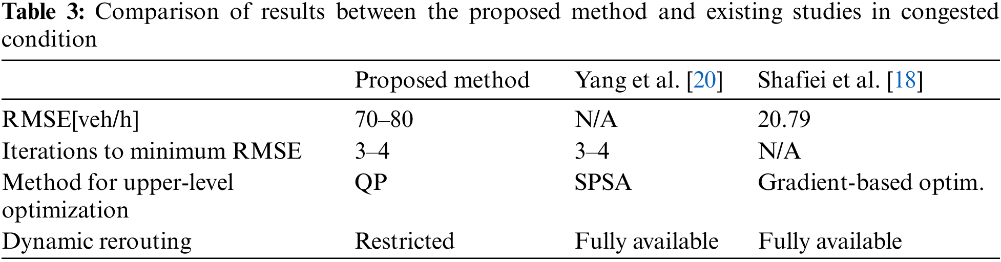
Figure 6: Change in RMSE for control, weak and strong cases

In all cases, the RMSEs were observed at the 3rd or 4th iteration step, and increased subsequently. This can be explained by the fact that congestion grew worse in later iterations. There were no significant differences among the cases in terms of their RMSE. The number of iteration steps needed to produce a feasible optimal result with the proposed method was nearly identical to that for Yang et al.’s method [20]. Considering that SPSA requires simulations twice as lower-level optimizations to calculate the gradient [27] and that simulation runs occupy a large portion of the estimation time (see also Subsection 6.2), the proposed method is computationally more efficient than Yang et al.’s method.

Figs. 7a–7c show scatter plots obtained from a trial whose RMSE was the median at the 4th iteration. The correlation and regression coefficients are sufficiently high and similar to those in the verification case. Therefore, the authors concluded that, the link traffic volumes were reproduced well as a whole. However, from a different perspective, the fact that the RMSE remains at approximately 80 veh/h shows a limitation of the application in its current stage. Some large differences between the simulated and the observed link traffic volumes were seen at various observation points, with differences of 463 and 61 representing the most remarkable examples (Fig. 7a). The reason for this is traffic volume drop due to congestion. Congestion detection leads to suppressing traffic volume on all links evenly. Thus, the RMSE can be improved only to a certain extent, as long as the entire reproducibility of the link traffic volumes across all links is limited. Further improvements require simulation parameters that more accurately describe driver behavior.

Figure 7: Scatter plots for cases with/without congestion detection with regression lines

Next, the results were compared to a study by Shafiei et al. [18] that used gradient-based optimization. Their method is also implemented offline and is nearly the same as the method described in Subsection 4.2 for preparing an initial OD matrix.

Shafiei et al. pointed out that if the gradient of the objective function was simply used for updating the OD matrix solution candidate, it would be invalid under congested conditions. Though their approach is similar to the congestion detection method employed in this research, as given in Eq. (8), they dealt with the problem by considering the results of a sensitivity analysis of link traffic volume to determine the assignment matrix A. In brief, they attempted to substitute Eq. (4) with a first-order Taylor approximation, similar to Eq. (11). Note that the assignment matrix A changes from a constant to a function of the OD vector x.

Q^j=Aj(x∗)+(∂Aj(x∗)∂xx∗)T(x−x∗).(11)

Here, subscript j denotes the index of the row, and the differential symbol denotes vector differentiation. x∗ is the current OD matrix candidate solution.

Shafiei et al. calculated the second term of Eq. (11) in partial rather than total terms. This operation is based on introducing the initial OD matrix into the objective function.

As a result of testing their approach on a small-scale network, Shafiei et al. obtained an RMSE of 20.79 in a heavy congestion scenario. Clearly, this is much smaller than the RMSE of 70–80 obtained in the present study. The authors consider that the difference arises from the dynamic rerouting feature implemented in the traffic simulator used by Shafiei et al. In terms of distributing demand, full dynamic rerouting affects each vehicle’s routing strategy dynamically, whereas the presently proposed method affects traffic volume statically outside the simulation. Therefore, the authors doubt that the larger RMSE for the proposed method arises from fictitious congestion occurring in the simulation. Subsection 6.1 clarifies the congestion behavior.

6  Discussion

6.1 Suppression Effect in Congestion

The change of the total number of stuck vehicles, which is calculated simply by summing all values for all links, is shown in Fig. 8.

Figure 8: Change in total number of stuck vehicles

Fig. 8 shows that there were fewer stuck vehicles in the Strong case than in the Control case. Although there was no statistically significant difference, in comparing the mean values at the 4th iteration step, the number of stuck vehicles is 12% less in the Strong case than in the Control case. This result shows that the proposed congestion detection successfully reduces the number of such vehicles under the situation employing restricted dynamic rerouting.

The results also show that the total number of stuck vehicles increases monotonically at each iteration in all cases. In iteration steps 1–4, since the total number of generated vehicles increases with each iteration, there is an increase in the total number of stuck vehicles. In later iteration steps, as noted in Subsection 5.2, there are many stuck vehicles and it is difficult to measure the true demand on the link because of the heavy congestion. In addition, the regression coefficient is always below 1.0, i.e., the renewal of the OD matrices in the estimation loop always leads to increased demand in some OD pairs. This renewal causes positive feedback for congestion. It is also noteworthy that the number of stuck vehicles increases greatly in these later iteration steps. Considering above, these results suggest that the maximum number of iterations kmax should be 5.

6.2 Computational Efficiency and Scalability

The authors used a simulator with restricted dynamic rerouting to reduce the computational time in the OD estimation process. The most calculation-expensive operation in the simulation is the route search. In Dijkstra’s algorithm, the origin of the A* algorithm, the worst-case time complexity is O(E+Vlog⁡V), where E and V are the numbers of links and nodes in the network, respectively. The A* algorithm is more efficient than Dijkstra’s method, but not to the extent that it significantly reduces the order of the time complexity. When invoked dynamic rerouting based on the A* algorithm, the computational cost is multiplied by the total traffic demand and the total number of rerouting operations per vehicle. Especially, the latter corresponds to the size of the network. Because driving on a larger network increases rerouting chance during driving. Though the computational complexity for this cannot be defined strictly, it can be formulated like O(NE(E+Vlog⁡V)) with some assumptions; The first assumption is that total traffic demand is proportional to the number of OD pairs. The second is that number of rerouting operations is proportional to the number of links.

Here, considering additional assumptions, the formulation is expressed like O(N2log⁡N). The assumptions are like below: First, the number of links is proportional to the number of nodes: O(E)=O(V). There is no significant variation in the number of links that connect to one node. Second, the number of the origin or destination nodes P is proportional to the total number of nodes: O(P)=O(V). Third, the number of the OD pairs is the total number of combinations of origin and destination nodes: O(N1/2)=O(P).

Quadratic programming was used in this study reduce the number of simulation runs in one iteration, and a majority of the computational time is consumed in the simulation portion of the procedure. For example, the mean values in one iteration of the Control case were 131.4 s in running simulation and 38.6 s in running QP solver. Even in the free-flow state, the computational time for the simulation predominates in the OD estimation. Our work supports that 75% of the computation time is spent in routing operation through a simulation run [36]. By introducing dynamic rerouting into the simulator, the computational time for the simulation is expected to be several times longer than in the Control case.

Here, Fig. 9 shows the relationship between computational time for QP and simulation. The red points indicate these typical values in the examined cases. Purple and green lines are the approximated computation time discussed above. This figure shows that if the number of nodes is smaller than about 400–500, the simulation time is lower than QP. This result suggests that when computing the OD estimation in a typical medium-sized city in Japan like this experiment, since the computational cost for simulation is larger than upper-level optimization, the proposed method has an effect in reducing calculation cost.

Figure 9: Estimated computational time for QP and simulation

When dealing with extremely large networks, the QP solver may take longer computational time than the simulation. The worst-case time complexity for the QP algorithm is roughly approximated as O(N3) under the assumption that the linear equations are solved with LU decomposition and that upper or lower bounds are not considered. These rough estimates show that the QP solver could potentially cause a bottleneck in the estimation procedure. However, it is worthwhile to reduce the simulation time by using the proposed method even for large networks where QP is dominant.

If we need to reduce the time for solving QP, reducing the number of variables is preferable. Since it is possible to conduct clustering for the results of a traffic simulation [37], a reduced-order estimation model can be developed using such a method.

7  Conclusions

In this paper, the OD estimation problem was formulated as a bi-level programming problem; the authors introduced congestion detection into the process of updating the OD matrices (upper-level optimization) to combine with a MAS-based microscopic simulator (lower-level optimization) with restricted dynamic rerouting. Because full dynamic rerouting functions are computationally expensive, restricted dynamic rerouting was used to reduce the computational cost. At the same time, a congestion detection was introduced to suppress excess traffic demand that cannot be treated well by the restricted dynamic rerouting. Although the congestion detection was combined with restricted dynamic rerouting, the method can also be applied to a simulator with full dynamic rerouting. The proposed congestion detection could reduce fictitious congestions that result from restricting dynamic rerouting. Test results showed that stuck vehicles were reduced by 12%. The reduction of fictitious congestion can improve the numerical stability of the entire estimation method.

Additionally, the reproducibility of link traffic volume using the proposed method proved to be nearly the same as that of existing methods. At the same time, the proposed method is computationally more efficient since the calculation cost of dynamic rerouting is reduced. This advantage is particularly evident when targeting wider-area or higher-demand conditions. However, the proposed method guarantees that reproducibility at the link without observation. It is required additional observation points or additional data source to fit the volume at such a link, velocities or other measurements. The authors regard it as for future task.

Importantly, the proposed method can be applied to any other traffic simulators that can output link traffic volume and the number of stuck vehicles. In addition, the proposed approach of adding information to the analysis may contribute to enhancing the efficiency of NN-based methods. For example, the authors have shown in the previous work [38] that a similar approach improves the efficiency of traffic state estimation in the event of a traffic incident using a graph convolutional recurrent neural network (GCRNN).

It would be prudent for future work to consider utilizing other observable traffic attributes as data sources for validation. For example, as described in Subsection 3.3, since the number of stuck vehicles corresponds to congestion length in the real world, it should be taken into account in the proposed method.

Acknowledgement: The first author was supported by the H-UTokyo Lab. Energy Project.

Availability of Data and Materials: The data that support the findings of this study are available from the corresponding author, K. Abe, upon reasonable request, except the observed traffic volume data. The observed traffic volume data are parts of the traffic survey result conducted by Fukui prefecture and the authors are permitted only to use them, not to distribute them. The simulator which is employed, ADVENTURE_Mates, is an open source software and is available at https://adventure.sys.t.u-tokyo.ac.jp/. Everyone can freely use this simulator for the purposes permitted under the simulator’s license and terms.

Funding Statement: This work was financially supported by JSPS KAKENHI (Grant Nos. 15H01785 and 19H02377).

Conflicts of Interest: The authors declare that they have no conflicts of interest to report regarding the present study.

References

1. McNally, M. G. (2007). The four step model, 2nd edition. Bingley: Emerald Group Publishing Limited. [Google Scholar]
2. van Zuylen, H. J., Willumsen, L. G. (1980). The most likely trip matrix estimated from traffic counts. Transportation Research Part B, 14(3), 281–293. DOI 10.1016/0191-2615(80)90008-9. [Google Scholar] [CrossRef]
3. Willumsen, L. G. (1984). Estimating time-dependent trip matrices from traffic. Ninth International Symposium on Transportation and Traffic Theory, pp. 397–411. Delft, Nederland: VNU Science Press Utrecht. [Google Scholar]
4. Teodorovic, D., van Aerde, M., Dion, F. (2002). Genetic algorithms approach to the problem of the automated vehicle identification equipment locations. Journal of Advanced Transportation, 36(1), 1–21. DOI 10.1002/atr.5670360102. [Google Scholar] [CrossRef]
5. Spiess, H. (1987). A maximum likelihood model for estimating origin-destination matrices. Transportation Research Part B, 21(5), 395–412. DOI 10.1016/0191-2615(87)90037-3. [Google Scholar] [CrossRef]
6. Cascetta, E., Nguyen, S. (1998). A unified framework for estimating or updating origin/destination matrices from traffic counts. Transportation Research Part B, 22(6), 437–455. DOI 10.1016/0191-2615(88)90024-0. [Google Scholar] [CrossRef]
7. Cascetta, E. (1984). Estimation of trip matrices from traffic counts and survey data: A generalized least squares estimator. Transportation Research Part B, 18(4–5), 289–299. DOI 10.1016/0191-2615(84)90012-2. [Google Scholar] [CrossRef]
8. Bera, S., Rao, K. V. K. (2011). Estimation of origin-destination matrix from traffic counts: The state of the art. European Transport-Trasporti Europei, 49, 3–23. [Google Scholar]
9. Dijkstra, E. W. (1959). A note on two problems in connexion with graphs. Numerische Mathematik, 1, 269–271. DOI 10.1007/BF01386390. [Google Scholar] [CrossRef]
10. Hart, P. E., Nilsson, N. J., Raphael, B. (1968). A formal basis for the heuristic determination of minimum cost paths. IEEE Transactions on Systems Science and Cybernetics, 4(2), 100–107. DOI 10.1109/TSSC.1968.300136. [Google Scholar] [CrossRef]
11. Fellendorf, M. (1994). Vissim, A microscopic simulation tool to evaluate actuated signal control including bus priority. Proceedings of the 64th ITE Annual Meeting, Dallas, USA. [Google Scholar]
12. Barceló, J., Casas, J. (2005). Dynamic network simulation with aimsun. Operations Research/Computer Science Interfaces Series, 31, 57–98. DOI 10.1007/b104513. [Google Scholar] [CrossRef]
13. Krajzwicz, D., Feld, C., Wagner, P. (2002). Sumo (simulation of urban mobility); An open-source traffic simulation. 4th Middle East Symposium on Simulation and Modelling, Dubai, UAE. [Google Scholar]
14. Yoshimura, S. (2006). MATES: Multi-agent based traffic and environment simulator-Theory, implementation and practical application. Computer Modeling in Engineering & Sciences, 11(1), 17–26. DOI 10.3970/cmes.2006.011.017. [Google Scholar] [CrossRef]
15. Fujii, H., Uchida, H., Yoshimura, S. (2017). Agent-based simulation framework for mixed traffic of cars, pedestrians and trams. Transportation Research Part C: Emerging Technologies, 85, 234–248. DOI 10.1016/j.trc.2017.09.018. [Google Scholar] [CrossRef]
16. Horni, A., Nagel, K. (2016). The multi-agent transport simulation MATSim. London: Ubiquity Press. [Google Scholar]
17. Nguyen, T., Krajzewicz, D., Fullerton, M. (2015). DFROUTER-estimation of vehicle routes from cross-section measurements. In: Modeling mobility with open data, pp.3–23. DOI 10.1007/978-3-319-15024-6. [Google Scholar] [CrossRef]
18. Shafiei, S., Saberi, M., Zicjauem, A., Sarvi, M. (2017). Sensitivity-based linear approximation method to estimate time-dependent origin-destination demand in congested networks. Transportation Research Record: Journal of the Transportation Research Board, 2669, 72–79. DOI 10.3141/2669-08. [Google Scholar] [CrossRef]
19. Spall, J. C. (1992). Multivariate stochastic approximation using a simultaneous perturbation gradient approximation. IEEE Transactions on Automatic Control, 37(3), 332–341. DOI 10.1109/9.119632. [Google Scholar] [CrossRef]
20. Yang, H., Wang, Y., Wang, D. (2018). Dynamic origin-destination estimation without historical origin-destination matrices for microscopic simulation platform in urban network. 21st International Conference on Intelligent Transportation Systems (ITSC), Maui, USA. [Google Scholar]
21. Djukic, T., Masip, D., Breen, M., Casas, J. (2017). Modified bi-level optimization framework for dynamic od demand estimation in the congested networks. Proceedings of Australasian Transport Research Forum, Auckland, New Zealand. [Google Scholar]
22. Balakrishna, R., Ben-Akiva, M., Koutsopoulos, H. (2007). Offline calibration of dynamic traffic assignment: Simultaneous demand and supply estimation. Transportation Research Record: Journal of the Transportation Research Board, 2003(1), 50–58. DOI 10.3141/2003-07. [Google Scholar] [CrossRef]
23. Cipriani, E., Florian, M., Mahut, M., Nigro, M. (2011). A gradient approximation approach for adjusting temporal origin-destination matrices. Transportation Research Part C: Emerging Technologies, 19(2), 270–282. DOI 10.1016/j.trc.2010.05.013. [Google Scholar] [CrossRef]
24. Omrani, R., Lina, K. (2018). Concurrent estimation of origin-destination flows and calibration of microscopic traffic simulation parameters in a high-performance computing cluster. Journal of Transportation Engineering, Part A: Systems, 144(1), 04017068. [Google Scholar]
25. Marzano, V., Papola, A., Simonelli, F., Papageorgiou, M. (2018). A kalman filter for quasi-dynamic o-d flow estimation/updating. IEEE Transactions on Intelligent Transportation Systems, 19(11), 3604–3612. DOI 10.1109/TITS.2018.2865610. [Google Scholar] [CrossRef]
26. Yonusefikia, M., Mamdoohi, A. R., Moridpur, S., Noruzoliaee, M. (2013). A study on the generalized tflowfuzzy od estimation. Proceedings of Australasian Transport Research Forum 2013, Brisbane, Australia. [Google Scholar]
27. Antoniou, C., Azevedo, C. L., Lu, L., Pereira, F., Ben-Akiva, M. (2015). W-Spsa in practice: Approximation of weight matrices and calibration of traffic simulation models. Transportation Research Part C, 59, 129–146. DOI 10.1016/j.trc.2015.04.030. [Google Scholar] [CrossRef]
28. Tang, K., Cao, Y., Yao, J., Tan, C., Sun, J. (2021). Dynamic origin-destination flow estimation using automatic vehicle identification data: A 3D convolutional neural network approach. Computer-Aided Civil and Infrastructure Engineering, 36(1), 30–46. DOI 10.1111/mice.12559. [Google Scholar] [CrossRef]
29. Koca, D., Schmöcker, J. D., Fukuda, K. (2021). Origin-destination matrix estimation by deep learning using maps with New York case study. 2021 7th International Conference on Models and Technologies for Intelligent Transportation Systems (MT-ITS), pp. 1–6. Heraklion, Greece. [Google Scholar]
30. Abe, K., Fujii, H., Yoshimura, S. (2017). Inverse analysis of origin-destination matrix for microscopic traffic simulator. Computer Modeling in Engineering & Science, 113(1), 71–87. DOI 10.3970/cmes.2017.113.068. [Google Scholar] [CrossRef]
31. Abe, K., Fujii, H., Yoshimura, S. (2019). Estimation of traffic demand corresponding to observed link traffic volume in microscopic simulation. 2019 IEEE Intelligent Transportation Systems Conference (ITSC), Auckland, New Zealand. [Google Scholar]
32. COIN-OR. Github-coin-or/qpoases: Open-source c++ implementation of the recently proposed online active set strategy. https://github.com/coin-or/qpOASES. [Google Scholar]
33. Treiber, M., Kesting, A. (2013). Traffic flow dynamics, data, models and simulation. Heidelberg: Springer. [Google Scholar]
34. US Department of Commerce (1964). Traffic assignment manual: For application with a large, high speed computer. Washington DC: Government Printing Office. [Google Scholar]
35. Treiber, M., Hennecke, A., Helbing, D. (2000). Congested traffic states in empirical observations and microscopic simulations. Physical Review E, 62(2), 1805–1824. DOI 10.1103/PhysRevE.62.1805. [Google Scholar] [CrossRef]
36. Kohashi, T., Bunya, S., Fujii, H., Yoshimura, S. (2010). Parallelization of intelligent multi-agent based traffic and environment simulator mates. Transactions of JSCES, 2010, 20100003 (in Japanese). [Google Scholar]
37. Yanai, M., Abe, K., Yamada, T., Fujii, H., Yoshimura, S. (2018). Cluster analysis for a series of microscopic traffic simulation results. Journal of Advanced Simulation in Science and Engineering, 4(1), 78–98. DOI 10.15748/jasse.4.78. [Google Scholar] [CrossRef]
38. Fukuda, S., Uchida, H., Fujii, H., Yamada, T. (2020). Short-term prediction of traffic flow under incident conditions using graph convolutional RNN and traffic simulation. IET Intelligent Transport Systems, 14(8), 936–946. DOI 10.1049/iet-its.2019.0778. [Google Scholar] [CrossRef]
Cite This Article
Copyright © 2023 The Author(s). Published by Tech Science Press.
This work is licensed under a Creative Commons Attribution 4.0 International License , which permits unrestricted use, distribution, and reproduction in any medium, provided the original work is properly cited.
Downloads
Citation Tools