
 Submit a Paper
 Propose a Special lssue
 Open Access
ARTICLE
Multidisciplinary Modeling and Optimization Method of Remote Sensing Satellite Parameters Based on SysML-CEA
1 School of Mechanical Engineering, Hangzhou Dianzi University, Hangzhou, 310018, China
2 State Key Laboratory of Digital Manufacturing Equipment and Technology, Huazhong University of Science and Technology, Wuhan, 430074, China
* Corresponding Author: Changyong Chu. Email:
(This article belongs to the Special Issue: New Trends in Structural Optimization)
Computer Modeling in Engineering & Sciences 2023, 135(2), 1413-1434. https://doi.org/10.32604/cmes.2022.022395
Received 29 March 2022; Accepted 20 June 2022; Issue published 27 October 2022
 View Full Text
 Download PDF
Abstract
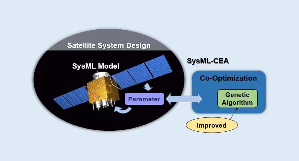
To enhance the efficiency of system modeling and optimization in the conceptual design stage of satellite parameters, a system modeling and optimization method based on System Modeling Language and Co-evolutionary Algorithm is proposed. At first, the objectives of satellite mission and optimization problems are clarified, and a design matrix of discipline structure is constructed to process the coupling relationship of design variables and constraints of the orbit, payload, power and quality disciplines. In order to solve the problem of increasing non-linearity and coupling between these disciplines while using a standard collaborative optimization algorithm, an improved genetic algorithm is proposed and applied to system-level and discipline-level models. Finally, the CO model of satellite parameters is solved through the collaborative simulation of Cameo Systems Modeler (CSM) and MATLAB. The result obtained shows that the method proposed in this paper for the conceptual design phase of satellite parameters is efficient and feasible. It can shorten the project cycle effectively and additionally provide a reference for the optimal design of other complex projects.Graphic Abstract
Keywords
Remote sensing satellite is a well-known large-scale complex system whose design process involves multiple disciplines, such as mission analysis, orbit, remote sensing payload, structures, attitude determination and control system, power, thermal, communication and command data (C&DH), etc. It is a conventional system engineering. Satellite system design [1–3] is to determine overall goal and constraints on the basis of mission demand analysis, and obtains a satellite design that can satisfy the requirements. Designers from various disciplines communicate and negotiate with each other in this process. Researches and developments of satellite model usually depend on the experience of designers while selecting the design alternatives based on design history inheritance [4–8].
The conventional mode of satellite system design is document-centric, which is also known as Text-Based Systems Engineering (TBSE). With the appearance of serious problems caused by large amounts of information and constantly revised data. The inefficiency of TBSE that relies on ordinary files or other unrelated storage has become an obstacle for satellite system design. Proofreading, modification, and evaluation are time-consuming and need too many iterations in the design cycle [9–11]. Moreover, requirements defined in documents or contracts often occur information missing or misunderstandings during the transmission in requirements analysis. Insufficient and in-depth understanding for user requirements makes repeated designs in the follow-up, or even causes the usage of satellites inconvenient.
Due to the high coupling between satellite subsystems, coordinating requirements and indicators are in trouble. In conceptual design, each subsystem can only obtain the best solution of a single discipline or a certain subsystem when the design optimization of each subsystem was carried out separately. If the optimization result changes, engineers who are responsible for the remaining subsystems would re-coordinate these indicators, which affect the research and development efficiency seriously. Moreover, there are too many conflicts between various disciplines in satellite system design, which may cause the optimization of the design scheme hardly converge to a unique solution and get a nonoptimal design. For example, thicker side panels in the satellite structure can increase safety, but thinner side panels are lighter, the balance between satellite quality and structural design is required. Hence, TBSE is no longer suitable for the analysis and design which become further complex. To deal with aforementioned challenges, Model-Based Systems Engineering [12] (MBSE) and multidisciplinary design optimization [13] (MDO) are proposed, which would solve the design problems of complex engineering systems.
Berrezzoug et al. [14] have researched the geostationary (GEO) communication satellite and proposed a gravity search algorithm based on the law of interaction between gravity and mass under the consideration of system performance indicators such as quality, size, cost, reliability, etc. The result shows that the total mass of the GEO communication satellite has been reduced by 185.3 kg. Wu et al. [15] have discussed the commonalities between overall satellite parameter optimization and MDO, and they established an optimization model for MDO-oriented earth observation satellite. Shi et al. [16] have proposed an agent-assisted MDO framework composed of multiple modules to solve the multi-disciplinary problem of GEO satellite. The results show that the total mass of the satellite designed under this optimization framework is reduced by 7.3%, as provided a valuable reference for the design of other spacecraft systems. Cencetti et al. [17] have studied the relevant content of the integrated design optimization framework in the MBSE and evaluate the feasibility, advantages and disadvantages of this connection. Hesse et al. [18] have used the MBSE method in research of the relationship between passenger aircraft vibration and cabin comfort. With this addition, the advantages of this method in overall cabin design gradually become prominent. Rocha et al. [19] have proposed a technology for process integration and design exploration in which test data can be stored on a common platform, and all components used in optimization could be traced to its source and target product. The result shows that the MBSE method is effective for the optimization design. Boggero [20] has established the structure, behavior, and parameter diagrams of System Modeling Language (SysML) in the research of MDO technology for spacecraft system research and development and constructed all the relationships between disciplines in terms of input and output. SysML and MDO in their research are loosely coupled and applied to the spacecraft requirement analysis and function combing stage to establish the connection between disciplines and the design workflow. Gray et al. [21] have proposed an open source MDO framework openMDAO, which takes advantage of state-of-the-art algorithms to solve coupled models.
The above research mainly focused on requirements analysis and function defining stage, and the connection between SysML and MDO is a “loose coupling”. While in this work, the main focus of SysML-based MDO is on the aspect of numerical processing, which runs through the entire design and optimization process. There are some tools developed to support MBSE in complex system design and modeling. However, none of them has got the functionality of supporting system optimization. There are some tools to support MDO, but none of them is integrated with design models in SysML. This work is motivated by this gap and aims to develop effective methods to support automatic system optimization for MBSE.
MBSE and MDO are both methods for designing complex products. They focus on modularity and coupling between multiple disciplines. In system analysis and design of aerospace, shipbuilding, and vehicles, the improvement of comprehensive performance of complex systems depends on coupling coordination between various disciplines. MBSE can describe and analyze the relationship between the product and its components from all aspects of the product life cycle formally and clearly, while the MDO method can achieve overall design optimization on the basis of model-based design. In this work, the MBSE model is used as an intermediate data model to facilitate the data exchange between different disciplines in analysis and improve the efficiency of resource optimization allocation and sharing. Meanwhile, it is more convenient than the process model in the previous MDO optimization strategy to process coupled information. However, there are relatively few researches on integrating the system model generated by the system design stage and the optimization model generated in the subsequent multidisciplinary optimization [22–25].
This paper proposes a modeling and optimization method for complex product and multidisciplinary system based on SysML and Co-evolutionary Algorithm (CEA) which aims to increase the efficiency of system modeling and optimization in the conceptual design phase of complex products. The method regard system objectives and optimization problems as a guide and establish an optimization model of efficiency evaluation indicators which involves quality analysis, track, payload, and power source disciplines. It uses Co-simulation by CSM and MATLAB for verification. The result shows that the improved genetic algorithm (GA) is more efficient at solving the multidisciplinary optimization problem on the basis of the SysML model after comparing and verifying the effectiveness and engineering value of the SysML-CEA method in the optimization of overall parameters of remote sensing satellites, and this method can also be applied in the design process of other complex products.
2 Optimization Model for Multidisciplinary Design of Remote Sensing Satellite
2.1 System Objectives and Optimization Issues
In this paper, the objective of the research and development mission for the remote sensing satellite is to monitor the forest fire situation and atmospheric environment in the Middle East, Africa and the regions between the north and south latitudes 40° in the world. The weight of the total satellite is required to be no more than 800 kg. Its orbit should achieve global coverage and meet energy security and it should have capabilities of camera imaging and image downloading with a resolution of less than 2.0 m. During orbit control, it is able to capture the initial attitude, and adjust inclination and orbit height. Before the orbit control, it can also perform a 90° roll/pitch attitude maneuver. In the process of orbit control, the attitude angle control accuracy is less than 3°. As for fuel configuration, it should meet the requirements for maintaining orbit and avoiding debris during the life, and de-orbit at the end of the life.
The acquisition of an index is one of the important parts in satellite design. Based on the concept of system engineering, indicators are defined and classified as measures of effectiveness (MOE), measures of performance (MOP) and technical performance measures (TPM). The MOE is used to measure the degree to which user needs are achieved in the system design, and establish a three-level index decomposition tree which consists of mission-level, system-level, and standalone-level. Index decomposition is necessary. On the one hand, index decomposition provides data support for the establishment of a multidisciplinary optimization mathematical model by using these indicators as parameters to measure the feasibility of the plan. On the other hand, these indicators can be decomposed into subsystems and standalone and used as value attributes to further perfect the logical architecture model. This paper focuses on analyzing the design of the key parameters that have a greater effect on the satellite design. It is the main content in the overall parameter design of the satellite which involves the disciplines like orbit, power, payload and quality. In this paper, the system’s optimization goals are determined by referring missions to remote sensing satellite and selecting important parameters as design variables. Hence, the method is universal.
According to the knowledge of the domain experts, an indicator decomposition tree in the system model is established by using these obtained indicators; it consists of task-level MOE, system-level MOP, and standalone-level TPM. MOE includes the observation area Coverage, imaging capability and quality (ICQ), satellite quality (mass), and Mission Life. MOP includes thirteen indicators such as local time of descending intersection (DNT), orbit height (h), Ground pixel resolution (GSD), signal-noise-ratio (SNR), Swath, etc. TPM includes sixteen indicators such as the quality of each subsystem, CCD camera focal length (f), battery capacity (Q), solar array windsurfing material type (Tsolar), camera spectrum range (Spectral Band), etc.
According to the index decomposition result in Fig. 1, the accumulated result of MOE is used as the objective function of the plan weighing. The subsystems decomposed into the index are the payload subsystem, power subsystem and attitude orbit control subsystem. Design variables include h, f, DNT, Q, T and A. While other subsystems and transmission variables involved are determined in accordance with conventional design experience so that it will not be reflected in the optimization process of this paper.
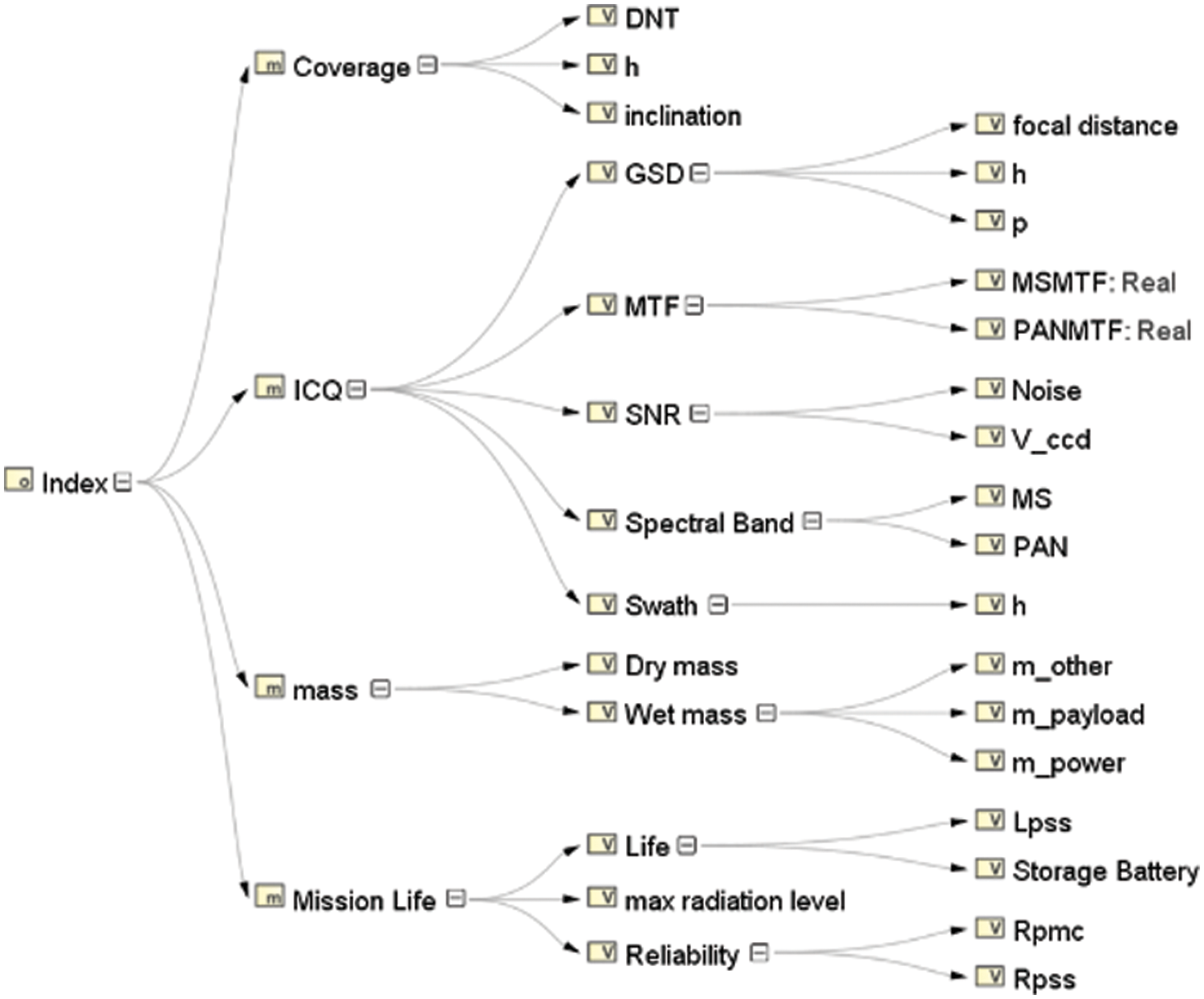
Figure 1: Satellite index breakdown diagram
In Eq. (1), X is the design variable. Wi is the weight coefficient of each design variable. F(X) is the system-level objective function. MOEi is the variable of each subsystem after quantification. Coverage is represented by center angle of observation coverage width ψ, ICQ is represented by GSD, and Mission Life is given by the demand that no less than 3 years. Mass is also given by the demand that no more than 800 kg. MOEi0 is a fixed value introduced for normalization.
According to the discipline analysis above, subsystems of the satellite are highly coupled and various parameters among different subsystems are related to each other. The coupling relationship among orbit, power, payload and mass are shown in the structural design matrix in Fig. 2. The horizontal line represents the subject output variable and the vertical line represents the subject input variable. While nodes represent coupling variables between disciplines.
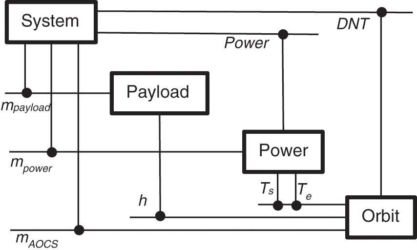
Figure 2: The satellite structure design matrix
2.2 Orbital Discipline Analysis
The orbit of the remote sensing satellite is sun-synchronous orbit. The output of the discipline parameter analysis includes Orbit period T, earth shadow time Te, and β, the angle between sunlight and array line of solar cell. In order to figure β, the first step is to calculate the right ascension and declination of the sun on the day because the incident angle of the sun changes with the variation of the sun’s position throughout the year.
In Eqs. (2) and (3), t presents the time and its value range is 0∼365. In the calculation of the right ascension of the sun, summer solstice is taken as the boundary and t takes 182.5. ε is the observation range of the north-south latitude of the subsatellite point. After the DNT is obtained, the right ascension of the ascending node of the satellite orbit can be converted as follows:
The angle between the sun’s rays and the orbital surface can be seen in the equation below:
In Eq. (5), i is the orbital inclination angle. If the angle between the solar cell array and the orbital plane is α, the angle between the sun’s rays and the normal of the solar array is β = γ − α.
Under the condition that the eclipse zone factor Ke is known, the earth shadow time can be obtained in the calculation below:
The orbital period T is calculated below:
In Eq. (7), Re is the earth’s equatorial radius (6371 km). μ is the gravity constant and μ = 3.986 × 10³ km3/s2. This discipline needs to meet the constraints of the sunshine duration Ts and the earth shadow duration Te.
The ground coverage area can be represented by ψ, the half center angle of the satellite observation coverage width.
In Eq. (9),
The output of power source parameter analysis includes solar array battery type, solar array output power, solar array area and battery pack rated capacity, etc. The type of solar array battery directly affects the design parameters, quality and area of the solar panel, and the system objective function would be affected indirectly. There are two kinds of batteries: silicon battery and gallium arsenide battery, they are represented as 0 and 1 respectively in the optimization. The power consumption of each subsystem can be divided into long-term power consumption P0 and short-term power consumption Ps. The minimum output power under a single-turn energy balance is Pc, and the required power PN of the solar array can be obtained
The long-term power consumption solar cell array needs to meet the charging power demand of the load and battery pack whose value is 649 W. The output power PBOL at the beginning of the battery life can be seen in the equation below:
In Eq. (11), S0 is the solar constant and S0 = 1353 W/m2. η is the single-chip photoelectric conversion efficiency of the solar battery. The value of η for silicon battery and gallium arsenide battery are 0.14 and 0.18, respectively. Fs is the combined loss factor of the solar batteries array with a value of 0.98. Ft is the temperature correction factor of the solar batteries array with a value of 0.48. A is the area of the solar batteries array. β is the angle between the sunlight and the normal line of the solar batteries array.
The mission requirement diagram demands that the satellite lifetime L should not less than 3 years. Due to the annual decline rate of the solar array’s output power being 2.2%, the output power at the end of the life can be calculated
The minimum rated capacity of the battery pack is calculated as follows:
In Eqs. (13) and (14), Qdischarg is the discharged power of the battery pack. DOD is the depth of discharge of a given battery pack with a value of 10.7%. PL is the long-term load power during the ground shadow period. Ps is the short-term load power during the ground shadow period. Vcell is the discharge voltage of the single battery. Ns is the number of battery cells connected in series. FLoss is the line loss factor.
The calculation of the mass of the battery and the solar panel is as follows:
In Eq. (15), Q is the battery capacity. VDB is the battery load voltage and the value is 28 V. ρac is the specific energy of the battery with a value of 39.6 W.h/kg.
In Eq. (16), ρsolar is the solar cell density and ρsolar = 2.6 kg/m2. A is the area of the solar windsurfing board. This discipline should satisfy the relationship between the output power PEOL and the battery capacity Q at the end of the life of the solar array as follows:
2.4 Payload Discipline Analysis
The payload of the remote sensing satellite in this paper is a five-band CCD camera whose image quality can be determined by two major parts: image radiation quality and geometric quality. Its evaluation indicators include ground pixel resolution, imaging width, spectral band configuration and ground observation angle. The input of the payload discipline analysis model is the orbit height and the focal length of the CCD camera. The output is camera quality, GSD, and SNR. GSD is the evaluation index of satellite geometric imaging quality. The main influencing factors are h, f, and p, which are calculated by the equation below:
In Eq. (18), the value of the pixel size p is 1.3 * 10–5 m. Meanwhile, GSD is directly proportional to h and inversely proportional to f. When the h and f decrease, the resolution of the ground pixel increases, and vice versa. Therefore, the design should choose a lower h and a higher f as much as possible in order to improve the GSD.
The quality and power of the CCD camera are related to the incident aperture, the estimation equations of them are as follows:
In Eqs. (19) and (20), mpayload is the quality of the CCD camera. Ppayload is the power consumption. dcam is the entrance aperture of the camera, its value is 1/4 of the f.
The spectral range is also a key indicator for satellite camera imaging. The spectrum range of the CCD camera generally selects a full chromatographic band and multiple multispectral bands in the range of 0.4 to 1.5 μm. The spectrum range of the CCD camera in this paper is 0.45∼0.52 μm, 0.52∼0.59 μm, 0.63∼0.69 μm, 0.77∼0.89 μm, 0.51∼0.73 μm.
On orbit signal-to-noise ratio (SNR) is the core evaluation index of satellite radiation imaging, which is the ratio of output image signal to noise. SNR can be solved by the following equation:
In Eqs. (21) and (22), VCCD is the output voltage of the CCD camera. VN1 and VN2 can be provided by the CCD device manual. VN3 and VN4 are as follows:
In Eqs. (23) and (24), ϑ is the charge output conversion efficiency. Vsat is the quantized saturation voltage, and QN is the number of quantized bits. The constraints that the discipline should satisfy are as follows:
3 Optimization Method for Multidisciplinary Design Based on SysML
3.1 The Main Content of MBSE-MDO
Model-based multidisciplinary design optimization (MBSE-MDO) is the inheritance and development of MDO on the basis of the MBSE system model. It obtains a set of engineering design variable that meet various constraints by exploring the coupling relationship between mathematical models, simulation analysis models and multi-disciplinary optimization models of these disciplines. The process of establishment of the SysML model in Fig. 3 is the reference source for the establishment of the multidisciplinary optimization design model which defines the mapping relationship between requirements, functions, parameters and structure of the remote sensing satellite system. It determines the stakeholder’s need and related constraints in the system model, which is conducive to the sensitivity analysis of the overall parameters of remote sensing satellites and improves the reliability of the discipline optimization model. In addition, the establishment process of the optimization model in Fig. 3 is carried out on the basis of the analysis models of these disciplines. The variables in the optimization process can be obtained through the decomposition of the efficiency indicators in system model and the coupling relationship between the variables would be simplified in line with mission demand and experience.
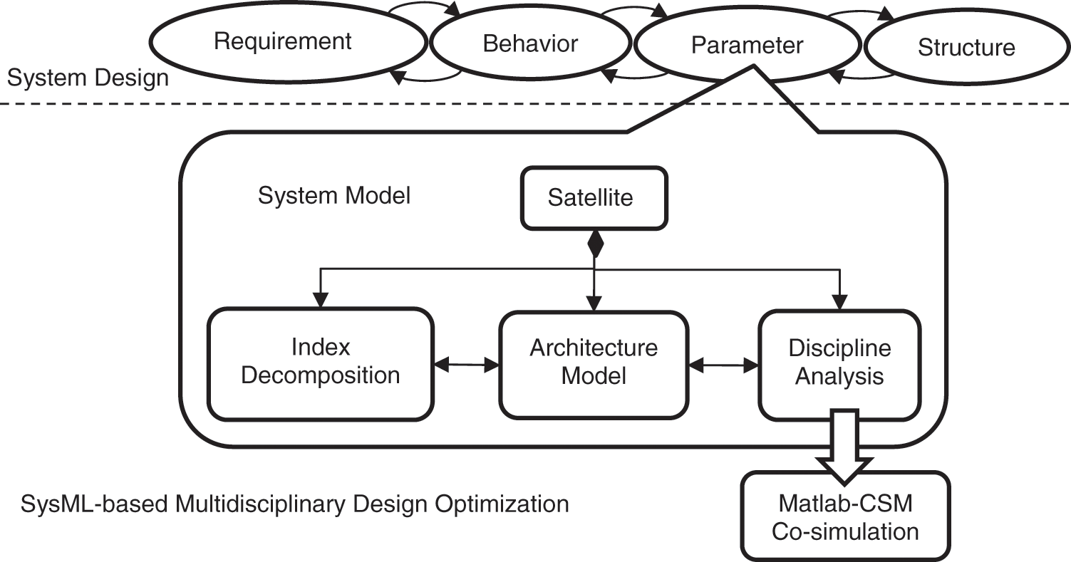
Figure 3: Comprehensive analysis and optimization method based on SysML
According to the features of data interaction, the system can be divided into hierarchical and non-hierarchical systems shown in Fig. 4 in order to choose a suitable optimization algorithm to solve the MDO problem easily. The structure of the hierarchical system is a tree structure in which the system at all levels can only exchange data with the upper system, and direct data interaction relationship between the same layer of systems does not exist. The non-hierarchical system does not have a fixed hierarchical relationship and data can be exchanged among these systems.
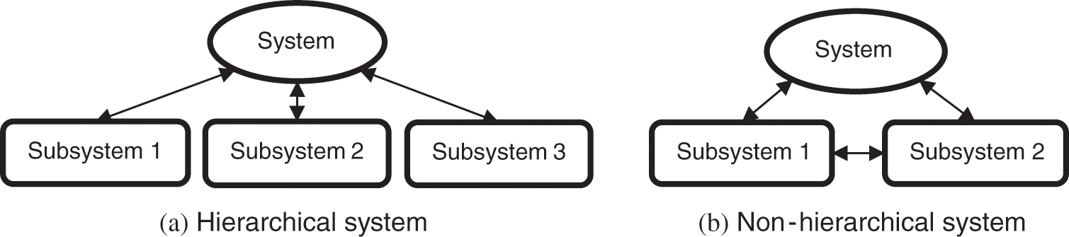
Figure 4: Hierarchical and non-hierarchical systems and their data interaction
Due to the different forms of organization in specific complex coupled design problems, MDO methods can be divided into two main groups: single-level optimization methods and multi-level optimization methods [26,27]. Single-level methods employ a single optimizer for the whole design problem which connects each discipline and analyzes and optimizes only at the system-level. Multi-level or distributed methods have the features of analysis and optimization that enables disciplinary autonomy. It decomposes complex design optimization problems into disciplines set (discipline-level) and manage interdisciplinary consistency by system-level coordination, which obtain the parallel inter-discipline optimization and coordinated optimization results between disciplines during system-level optimization. Typical single-level optimization methods include multiple discipline feasible method, individual discipline feasible method and all-at-once method. Multi-level optimization methods include concurrent subspace optimization method (CSSO) [28,29], collaborative optimization method (CO) [30–32], bi-level integrated system synthesis (BLISS) [33] and analytical target Cascading method (ATC) [34].
The disciplines such as orbit, payload, power and quality that mentioned in this paper have complex coupling relationships, which belong to a non-hierarchical system. The optimization problem in this paper requires analysis and optimization of each discipline-level module, so that the single-level optimization method is not used. The CSSO method requires the introduction of proxy model technology but all of the discipline model for the optimization problem in this paper are engineering estimation models. The ATC method is suitable for solving the distributed decision-making problem of the hierarchical structure [35] rather than the non-hierarchical system optimization problem. The BLISS method would obtain the sensitivity information from the coupled multidisciplinary system, which is very time-consuming. The CO method decomposes the optimization problem, which features small data transmission, high discipline autonomy, and a simple algorithm structure [36]. Hence, the CO method is chosen to optimize the design of the satellite’s parameters in this paper.
3.2 Collaborative Optimization Algorithm
CO algorithm is one of the methods applied to solve MDO problems which has been widely used in complex engineering problems. However, the CO algorithm has some defects. It usually falls into local solutions or cannot converge in nonlinear programming problems, causing multiple locally optimal solutions when meeting the nonconvex or even discontinuous design space of optimization problems in actual engineering problems. The multi-level optimization problem of CO research needs to establish two-level models: system level and subsystem level. The constraints at the system-level are the optimal target value after subsystem optimization and the optimal target value at the system-level can be obtained only when it meets the consistency constraints. The empty feasible region of the system level optimization model is inevitable, which makes the optimal design solution could not be obtained [37].
CO algorithm solves MDO problem by applying hierarchical strategy to decompose the complex system problem into multiple discipline-level problems and using a system-level optimization model to coordinate the discipline-level optimization results. The CO framework is shown in Fig. 5. The process of the solution is to minimize the D-value between the design optimization plan of discipline-level and system-level by the establishment of system-level and subsystem-level optimizers.
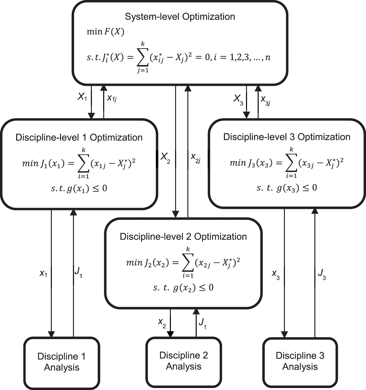
Figure 5: Collaborative optimization framework
(1) System-level mathematical model
In Eq. (26), X is the system-level design variable. The upper and lower boundaries are XL and XU. F(X) is the system-level optimization objective function. xij* is the optimal value of the j-th shared design variable at the i-th discipline-level. Xj is the j-th design variable at system-level. k is the number of discipline-level model. Ji*(X) is constraint conditions of the consistency equation provided for the i-th discipline.
(2) Discipline-level mathematical model
In Eq. (27), Ji(xi) is the optimization objective function of discipline-level Ji*. xij is the j-th design variable of the i-th subject level. Xj* is a system-level transmission variable. g(xi) is the discipline constraint function.
The organizational structure of the CO model is consistent with actual problems, and the information exchange between different disciplines is required to simplify. However, the standard CO algorithm is prone to absent the Lagrange multipliers in the system-level optimization and difficult to satisfy Kuhn-Tucker [38], which causes difficulties in optimization convergence. In order to improve the convergence of the CO algorithm, a modern intelligent optimization algorithm for solving the CO model is proposed in this paper. This algorithm does not require the mathematical model and derivative information of the optimization problem and can improve the convergence of optimization result.
A detailed analysis of the CO algorithm is shown in the section above. It can be seen that the nonlinear enhancement caused by the system decomposition and the complex coupling between disciplines led to the computational difficulties of the algorithm. The SysML-CEA algorithm can achieve collaboration among multiple disciplines by establishing a collaborative framework and integrating all the way of available discipline analysis (such as modules, tools, codes, etc.) which can solve MDO problems. SysML-CEA is a co-evolutionary algorithm based on SysML, which uses the improved GA [39] to search and optimize the two-level model of the CO algorithm to reduce the continuity and conductivity requirements of the optimization problem. The steps of the solution in the algorithm include the treatment of the CO model, the encapsulation of SysML constraint blocks and the application of improved GA optimization. The block definition diagram and parameter diagram in Fig. 6 contain the system-level and subject-level mathematical models for the optimization problem. The block and constraint block are shown in the left picture, the binding between values and parameters in the module is shown in the right picture. The data to be optimized is temporarily contained in the block after establishing the SysML model, which completes the preprocessing of the algorithm and performs the iterative solution later.
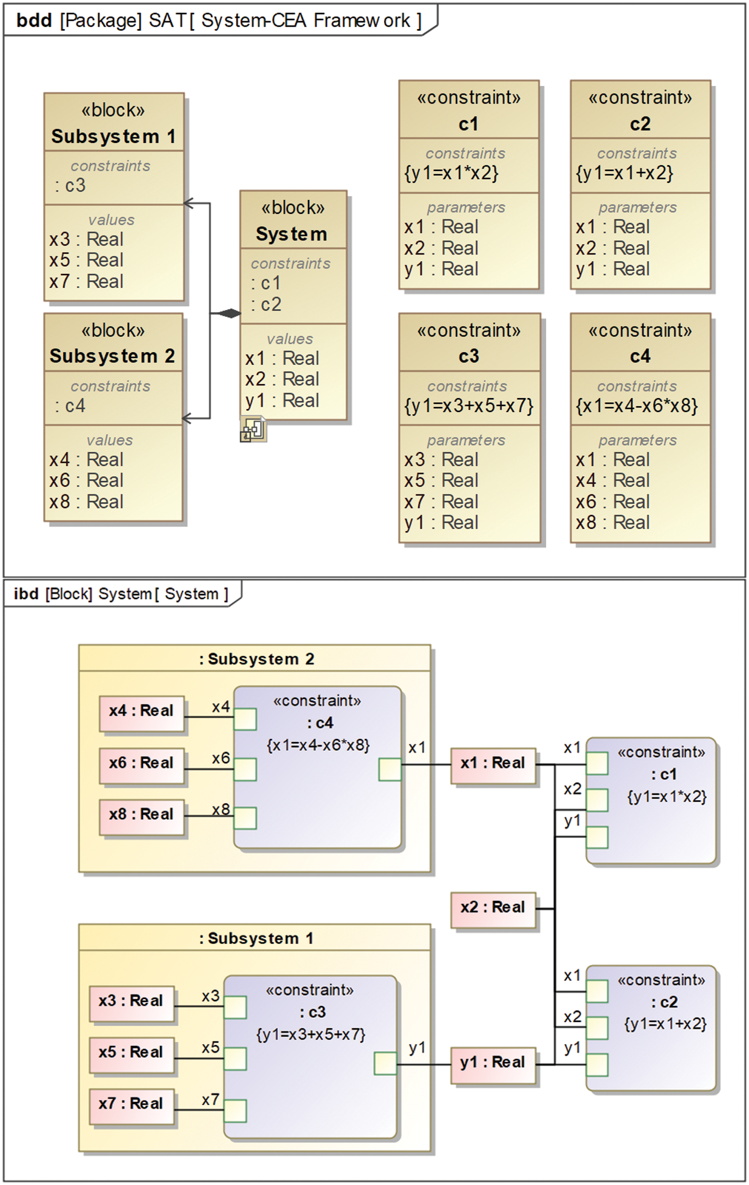
Figure 6: Collaborative optimization model in SysML model
System-level and discipline-level iterators use the improved GA to solve the problem represented by the model. Selection, crossover, and mutation operations in GA are improved to fix the numerical solution in multidisciplinary optimization in this section.
(1) Select operation
In selection operation, several chromosomes are selected from the primary population to form a new population and then obtain a convergent population finally after enough iterations in which the fitness value of chromosomes in this population will tend to the optimal solution. The most commonly used method for the chromosome probability calculation is the roulette selection method while the improved selection operation uses the best retention strategy after roulette selection to completely retain the chromosomes with the highest fitness in the population to the next generation.
(2) Cross operation
In crossover operation, the improved crossover pairs individuals with low fitness and low fitness, and pairs with high fitness and high fitness. Chaotic sequences [40] is adopted to determine the crossover positions of genes in chromosomes. If the crossover operation is performed on chromosomes U1 (λ12, λ22, λ32, …λ102) and U2 (λ12, λ22, λ32, …λ102), the chaotic sequence would be used in form of the equation below:
In Eq. (28), xn is the initial value randomly generated in (0∼1). xn+1 is the initial value of the chaos iteration of the next generation. The chaos value generated in each generation is kept and multiplied by 10 to get the locus in the chromosome.
(3) Mutation operation
The mutation operation is the operation that mutate the target value of a certain segment of genetic gene on the chromosome, which would generate a new chromosome. By pre-setting the mutation rate of the gene, the position of the mutation gene would selected randomly. An improved mutation operator is applied to ensure that the optimal chromosome mutation rate changes adaptively during the process of solution. The improved adaptive mutation rate is shown as follows:
In Eq. (29), Pm is the mutation rate, with a value that ranging from 0.0001 to 0.1. Pmax and Pmin are the upper and lower bounds of the value. kmax is the maximum genetic algebra.
The improved GA is adopted to optimize the two-level model of CO respectively as the step below. First, the discipline-level optimizer obtains the input variable of the discipline from the system-level optimizer and uses it as a fixed value in the optimization of the discipline. Secondly, variables of discipline-level design are combined for analyzing to obtain the discipline output variables, constraint values, and the D-value between discipline design variables and system-level design variables. The optimization goal is to minimize the D-value under the premise of satisfying the constraints. Finally, the system-level optimizer coordinates the D-value between these disciplines. The process of solution is shown in Fig. 7.
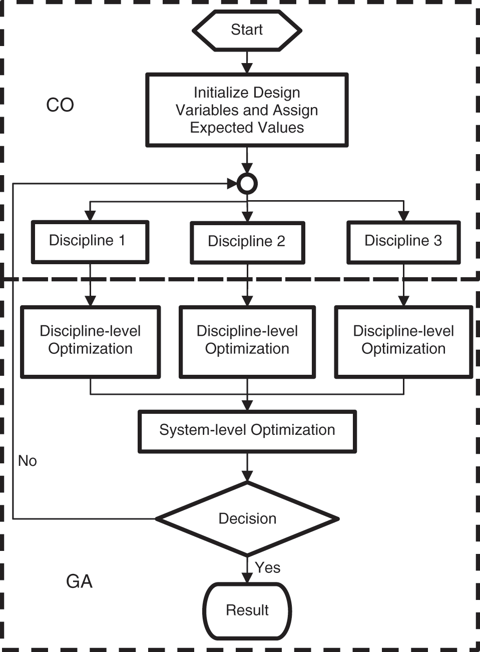
Figure 7: SysML-CEA solving process
Step 1: Design variables are initialized and expected values are assigned to the discipline-level optimizer. The initial value of the design variables, the constraint value, and the maximum number of iterations of the model are defined based on the demand of the problem.
Step 2: The discipline-level optimizer receives the input optimizer optimization indicators and combines these design variables of the system. GA is used in optimization to obtain the optimization results of design variables in the subsystem.
Step 3: GA parameters in Step 2 which include population, number of individuals, chromosome length, and genetic generation number are assigned. The operation of the genetic operator is performed to obtain the individual with the greatest fitness.
Step 4: After the completion of the optimization of each discipline, the optimal target value Ji is transmitted to the system-level optimizer and Ji* (X) = 0 is adopted as the constraint in optimization. The system-level optimization coordinates the inconsistency of optimization result at each discipline-level.
Step 5: Whether the consistency constraints meet the condition would be judged. If they meet the condition, the algorithm would finish the iterative process and get the result. Otherwise, it would return to Step 2 to continue execution.
4 Example of Optimization for Multidisciplinary Design of Remote Sensing Satellites
4.1 Satellite Multidisciplinary Collaborative Optimization Model
(1) System-level mathematical model
In Eq. (30), X is the design variable. Wi is the weight coefficient. F(X) is the system-level objective function. MOEi is the variable of each subsystem after quantification. MOEi0 is a fixed value introduced for normalized, gi* (X) is the system-level constraint of CO, which means it is the minimum value of the sub-system objective function in CO.
(2) Orbit discipline-level model
In Eq. (31), h is the shared system-level design variable. DNT, ψ are discipline-level design variables of this discipline. β, Te are coupled state variables and the output of this discipline which required by power supply discipline.
(3) Payload discipline-level model
In Eq. (32), h is the shared system-level design variable. f is the discipline-level design variable of this discipline. Ppayload is the coupling state variable which input by the power supply discipline. mpayload is the coupling state variable and the output of this discipline which required by quality discipline.
(4) Power discipline-level model
In Eq. (33), h is the shared system-level design variable. A, Q, Tsolar is the discipline-level design variable of this discipline. mac, msolar is the coupled state variable and the output of this discipline required by the quality discipline.
The normalization method [41] is adopted to process variables which can make the CO model more stable in solution and more convenient to obtain the optimal solution. Variables which in the range of 102∼103 such as orbit height, required power, and satellite quality are all reduced by 102 times. While variables with a range of 10∼102 are reduced by 10 times. Variables in range of 0∼10 are taken the original value. Due to the condition for the constraints of the original equation are stringent and hard to satisfy, the algorithm is adjusted in this paper for which the new condition is that gi* (xi) is less than 0.001. Equality constraints after adjusted are as follows:
CSM enables to perform calculation based on the parameter diagram of the system model. It contains a built-in script compiler that can implement languages such as JavaScript and Python and execute simple mathematical models. However, standard library files in CSM are insufficient and cannot use mature discipline analysis codes. By integrating the Matlab into the CSM, the usage of the M file is realized and the calculation of the CO model is completed, as Fig. 8 shows.
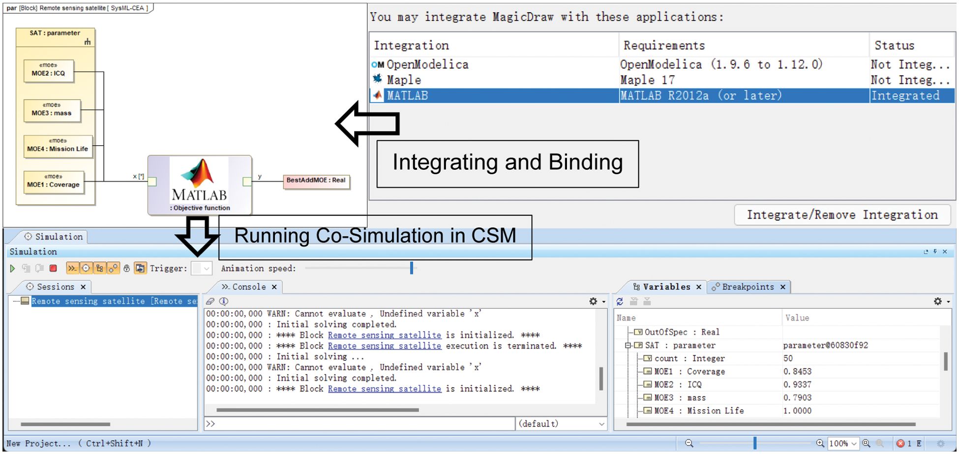
Figure 8: The calculation process of the optimization module under the CSM platform
In standard CO algorithm the two-level model is solved by the sequential quadratic programming (SQP) algorithm and GA while in SysML-CEA algorithm it is solved by the improved GA. In order to ensure the accuracy of the D-value between two optimization results, several consecutive optimizations are performed as follows:
(1) The optimization model of satellite multidisciplinary design is determined on the basis of actual needs to ensure that the system optimization target is the maximum of index of user requirements and it includes system-level design variables, discipline-level design variables, constraints, and several coupling state variables in these disciplines. Expected values of the subject-level optimization model are assigned in initialization and the population size of the GA is set to 50, the maximum genetic algebra is set to 60, and the maximum number of models call for CO is set to 100.
(2) The discipline optimizer of orbit, payload and power disciplines is executed respectively, and the improved GA is used to search and optimize the discipline objective function. After the optimization, the objective function value of the discipline is returned to the system-level optimizer as a constraint, and the optimal value of design variables of each discipline is returned at the same time.
(3) After the objective function and design variables from the discipline-level are received by the system-level optimizer, it searches and optimizes the objective function and updated system-level design variables are obtained as the input of the discipline analysis model to continue on the optimization.
(4) Whether the maximum number of calls to the discipline model is reached is judged in this step. If it is reached, the iteration and output the current optimal solution would be stopped. Otherwise, the workflow would return to Step (2) and continue with the next iteration until the optimization process is completed.
The satellite CO model is optimized and solved separately and the optimization results are shown as follows. The system objective function value result in Fig. 9 and the system-level consistency constraints in Fig. 10 show that the constraint value of standard CO algorithm tends to be near 5 * 10−4 in the fifth iteration and satisfies system consistency constraints so that the first set of optimized design variables is obtained. Due to the solving process applying the hierarchical solution strategy of the CO method, the objective function approximates the result only when the three disciplines satisfy the consistency constraint at the same time. The objective function value tends to converge after ten iterations. In contrast, the SysML-CEA algorithm satisfies the consistency constraint in the fourth iteration and the objective function value is converged after the eighth iteration, which means the efficiency is significantly better than the standard CO algorithm. In the iteration of SysML-CEA algorithm, the improved GA adopted by the optimizer performs a large-scale search on the solution set. In order to prevent falling into the local optimum when searching out the solution near the optimal value, an adaptive mutation rate is set in this paper. Fig. 9 shows that the curve fluctuates greatly in the initial stage of the algorithm iteration and tends to be stable in the later stage, which verifies the effectiveness of the adaptive mutation rate.
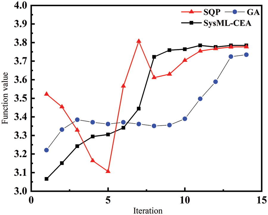
Figure 9: System-level objective function iteration curve
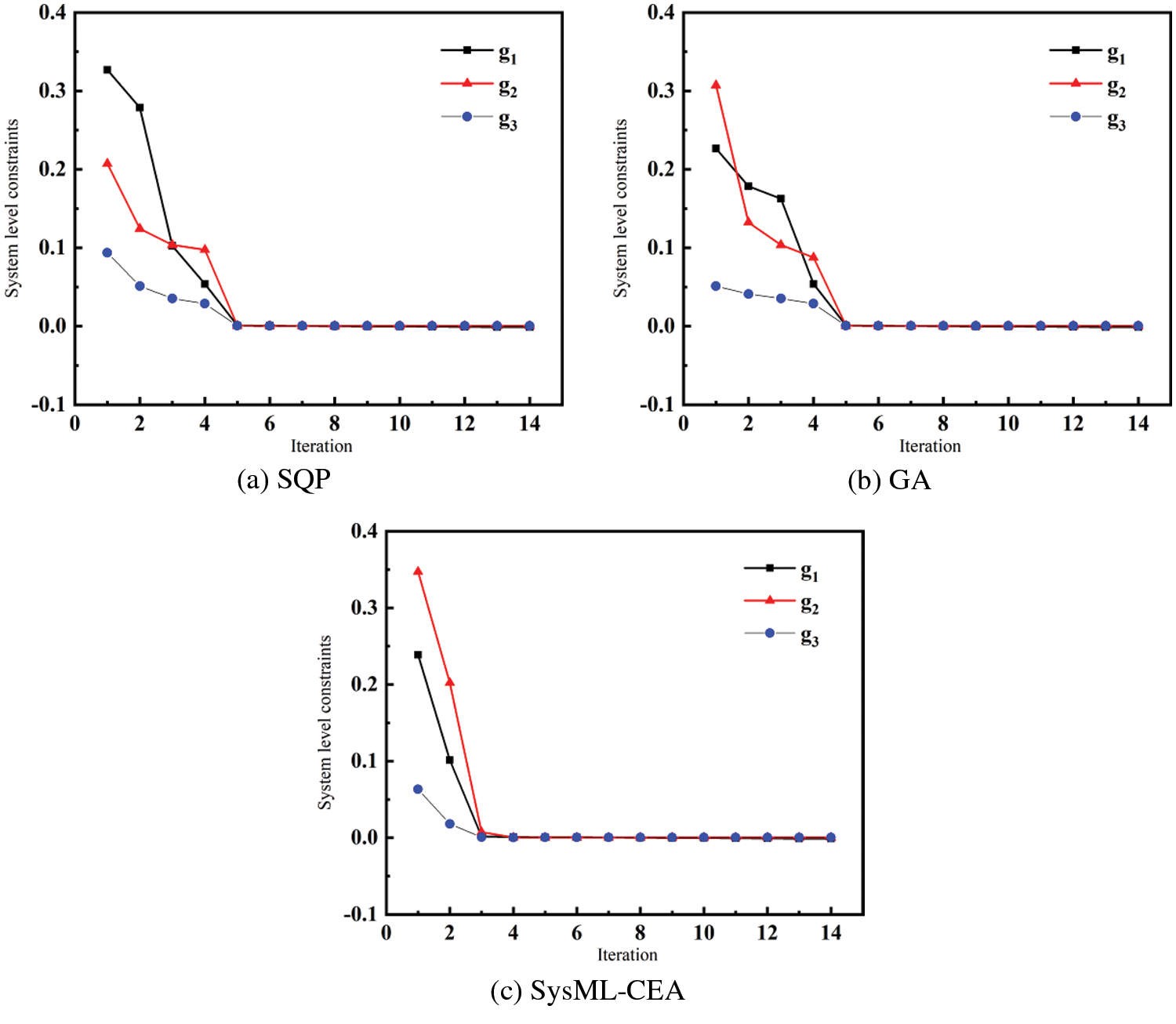
Figure 10: System-level constraint iteration curve (a) SQP (b) GA (c) SysML-CEA
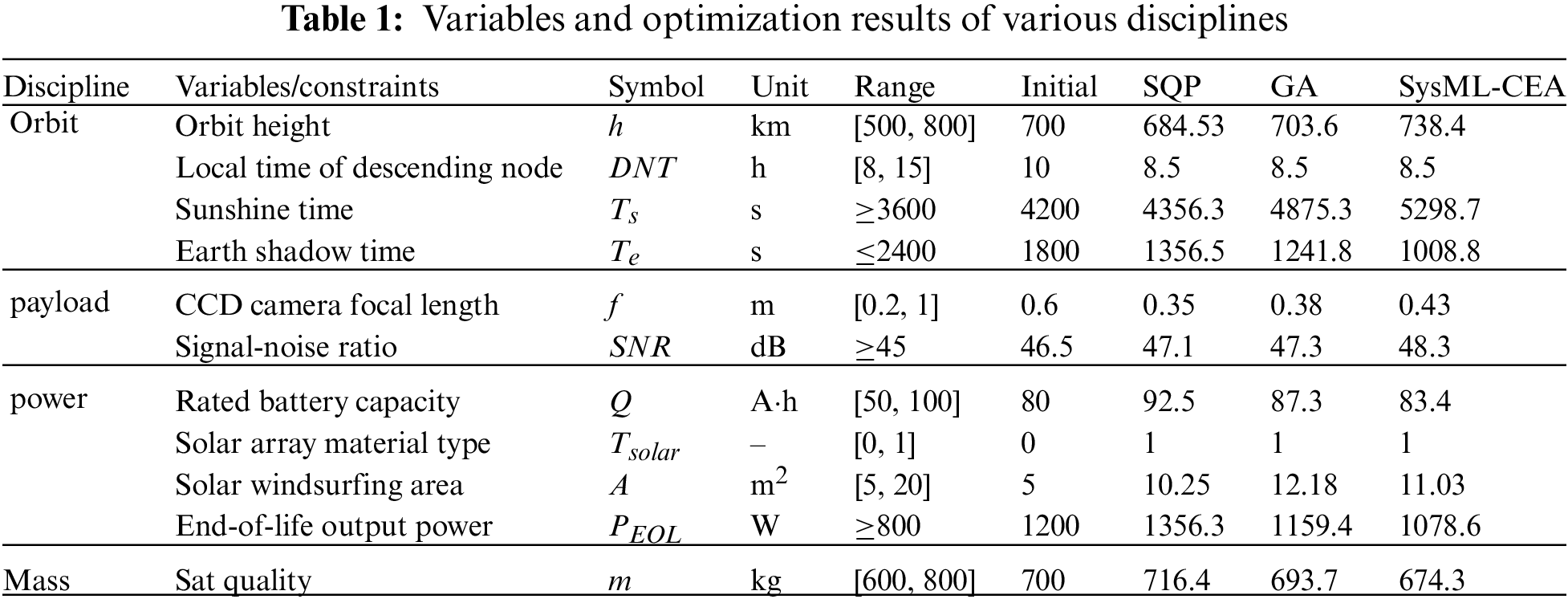
Table 1 shows that the optimization results of the standard CO algorithm and the SysML-CEA algorithm are both within the upper and lower bounds. Optimization results of these two discrete design variables of DNT and
This paper proposes an MDO based on MBSE for remote sensing satellite models’ research and development tasks. Analysis modeling and multidisciplinary coupling analysis for the orbit, payload, power supply and quality disciplines are completed. The SysML-CEA algorithm solution of the multidisciplinary optimization model is researched and the importance of the integration of MBSE and MDO in satellite conceptual demonstration and program design is confirmed.
The coupling relationship of the design variable related to subsystems in the MDO optimization problem is sorted out and the overall optimization objective function is established, which is based on the research mission and discipline knowledge of remote sensing satellite. The index variables are assigned to the corresponding discipline by the establishment of a three-level index decomposition tree. Based on the MBSE system model and discipline analysis model for multi-discipline design optimization, a co-evolutionary algorithm based on SysML is proposed. An improved GA that can solve two levels of the CO model is proposed to deal with problems of nonlinearity and coupling enhancement in discipline decomposition. The efficiency of the SysML-CEA algorithm in satellite multidisciplinary optimization design is verified by comparing the solution process.
The MDO method based on SysML has good expansibility. In addition to being applied to the remote sensing satellite in this paper, it can also be used to solve the design problems of other complex products. SysML MDO method can effectively save the time of information processing and integrate the computing strategy into one platform for processing, and facilitate information transmission.
Funding Statement: This work was supported by Open Fund of State Key Laboratory of Digital Manufacturing Equipment and Technology of China (Grant No. DMETKF2022015).
Conflicts of Interest: The authors declare that they have no conflicts of interest to report regarding the present study.
References
1. Muvuna, J., Boutaleb, T., Baker, K. J., Mickovski, S. B. (2019). A methodology to model integrated smart city system from the information perspective. Smart Cities, 2(4), 496–511. DOI 10.3390/smartcities2040030. [Google Scholar] [CrossRef]
2. Zadeh, P. M., Shirazi, M. S. (2017). Multidisciplinary design optimization architecture to concurrent design of satellite systems. Journal of Aerospace Engineering, 231(10), 1898–1916. [Google Scholar]
3. Prasanna Kumar, R. N., Patil, S. (2019). A system and method for improving the model based systems engineering environment capability. INCOSE International Symposium, 29(S1), 277–290. DOI 10.1002/j.2334-5837.2019.00685.x. [Google Scholar] [CrossRef]
4. Hause, M. C., Day, R. L. (2019). Frenemies: OPM and SysML together in an MBSE model. INCOSE International Symposium, 29(1), 691–706. DOI 10.1002/j.2334-5837.2019.00629.x. [Google Scholar] [CrossRef]
5. Biggs, G., Post, K., Armonas, A., Yakymets, N., Juknevicius, T. et al. (2019). OMG standard for integrating safety and reliability analysis into MBSE: Concepts and applications. INCOSE International Symposium, 29(1), 159–173. DOI 10.1002/j.2334-5837.2019.00595.x. [Google Scholar] [CrossRef]
6. Halstenberg, F. A., Stark, R. (2019). Study on the feasibility of modelling notations for integrated product-service systems engineering. Procedia CIRP, 83, 157–162. DOI 10.1016/j.procir.2019.02.133. [Google Scholar] [CrossRef]
7. Yuan, W., Wang, B., Chen, B., Qin, F., Shao, Y. (2020). Intelligent and efficient solution generation enabled by MBSE in high voltage system domain of EMU. Journal of Computer-Aided Design and Computer Graphics, 32(6), 979–988. [Google Scholar]
8. Mao, N. (2020). Development method of second power controller based on 6 V model’ MBSE. Aeronautical Computing Technique, 50(1), 105–109. [Google Scholar]
9. Wach, P., Salado, A. (2019). Can Wymore’s mathematical framework underpin SysML? An initial investigation of state machines. Procedia Computer Science, 153, 242–249. DOI 10.1016/j.procs.2019.05.076. [Google Scholar] [CrossRef]
10. Salado, A., Wach, P. (2019). Constructing true model-based requirements in SysML. Systems, 7(2), 19. DOI 10.3390/systems7020019. [Google Scholar] [CrossRef]
11. Vazquez-Santacruz, J. A., Torres-Figueroa, J., Portillo-Velez, R. D. J. (2019). Design of a human-like biped locomotion system based on a novel mechatronic methodology. Concurrent Engineering Research and Applications, 27(3), 249–267. DOI 10.1177/1063293X19857784. [Google Scholar] [CrossRef]
12. Madni, A. M., Sievers, M. (2018). Model-based systems engineering: Motivation, current status, and research opportunities. Spacecraft Engineering, 21(3), 172–190. DOI 10.1002/sys.21438. [Google Scholar] [CrossRef]
13. Afonso, F., Vale, J., Lau, F., Suleman, A. (2017). Performance based multidisciplinary design optimization of morphing aircraft. Aerospace Science and Technology, 67, 1–12. DOI 10.1016/j.ast.2017.03.029. [Google Scholar] [CrossRef]
14. Berrezzoug, S., Boudjemai, A., Bendimerad, F. T. (2019). Interactive design and multidisciplinary optimization of geostationary communication satellite. International Journal on Interactive Design and Manufacturing, 4(13), 106–113. DOI 10.1007/s12008-019-00590-7. [Google Scholar] [CrossRef]
15. Wu, B., Huang, H., Wu, W. (2011). Multidisciplinary design optimization of main parameters of spacecraft with sub-vehicles. Acta Aeronautica ET Astronautica Sinica, 32(4), 628–635. [Google Scholar]
16. Shi, R., Liu, L., Long, T., Liu, J., Yuan, B. (2017). Surrogate assisted multidisciplinary design optimization for an all-electric GEO satellite. Acta Astronautica, 138, 301–317. DOI 10.1016/j.actaastro.2017.05.032. [Google Scholar] [CrossRef]
17. Cencetti, M., Maggiore, P. (2013). System modeling framework and MDO tool integration: MBSE methodologies applied to design and analysis of space system. AIAA Modeling & Simulation Technologies, USA. [Google Scholar]
18. Hesse, C., Biedermann, J. (2019). Acoustic evaluation and optimization of aircraft cabin concepts--A systems engineering approach. International Workshop on Aircraft System Technologies, Germany. [Google Scholar]
19. Rocha T., Trmnen M. (2017). Multi-disciplinary optimization using model-based systems. NAFEMS World Congress, Sweden. [Google Scholar]
20. Boggero, L. (2018). Design techniques to support aircraft systems development in a collaborative MDO environment (Ph.D. Thesis). Politecnico Di Torino, Italy. [Google Scholar]
21. Gray, J. S., Hwang, J. T., Martins, J. R., Moore, K. T., Naylor, B. A. (2019). OpenMDAO: An open-source framework for multidisciplinary design, analysis, and optimization. Structural and Multidisciplinary Optimization, 59(4), 1075–1104. DOI 10.1007/s00158-019-02211-z. [Google Scholar] [CrossRef]
22. Zheng, G. (2019). Research on satellite constellation design and routing based on multi-objective optimization (M.S. Thesis). Chongqing University of Posts and Telecommunications, China. [Google Scholar]
23. Chen, Z., Lei, C., Gong, G., Li, N., Tian, C. et al. (2020). Key issues and methodology on cross-field co-design of complicated electronic information system dominated by effectiveness. Journal of Chinese Academy of Electronic Sciences, 15(5), 403–414. [Google Scholar]
24. Keskin, B., Salman, B. (2020). Building information modeling implementation framework for smart airport life cycle management. Transportation Research Record, 2674(6), 98–112. DOI 10.1177/0361198120917971. [Google Scholar] [CrossRef]
25. Cárdenas, R., Arroba, P., Blanco, R., Malagón, P., Risco-Martín, J. et al. (2020). Mercury: A modeling, simulation, and optimization framework for data stream-oriented IoT applications. Simulation Modelling Practice and Theory, 101, 102037. DOI 10.1016/j.simpat.2019.102037. [Google Scholar] [CrossRef]
26. Alexandrov, N. M., Hussaini, M. Y. (1997). Multidisciplinary design optimization: State-of-the-art. SIAM Journal on Control and Optimization, 1, 22–44. [Google Scholar]
27. Kodiyalam, S., Sobieszczanski-Sobieski, J. (2001). Multidisciplinary design optimization: Some formal methods, framework requirement and application to vehicle design. International Journal of Vehicle Design, 25, 3–32. DOI 10.1504/IJVD.2001.001904. [Google Scholar] [CrossRef]
28. Sobieszczanski-Sobieski, J. (1988). Optimization by decomposition: A step from hierarchic to non-hierarchic systems. NASA/Air Force Symposium on Recent Advances in Multidisciplinary Analysis and Optimization, USA. [Google Scholar]
29. Bloebaum, C. L., Hajela, P., Sobieszczanski-Sobieski, J. (1992). Non-hierarchic system decomposition in structural optimization. Engineering Optimization, 19, 171–186. DOI 10.1080/03052159208941227. [Google Scholar] [CrossRef]
30. Chagraoui, H., Soula, M. (2020). Multidisciplinary collaborative optimization based on relaxation method for solving complex problems. Concurrent Engineering, 28(4), 280–289. DOI 10.1177/1063293X20958921. [Google Scholar] [CrossRef]
31. Braun, R. (1996). Collaborative optimization: An architecture for large-scale distributed design (Ph.D. Thesis). Stanford University, USA. [Google Scholar]
32. Braun, R., Gage, P. J., Kroo, I. M., Sobieski, I. (1996). Implementation and performance issues in collaborative optimization. AIAA/USAF/NASA/ISSMO Multidisciplinary Analysis and Optimization Symposium, USA. [Google Scholar]
33. Sobieszczanski-Sobieski, J., Agte, J. S., Sandusky Jr, R. R. (2000). Bilevel integrated system synthesis. AIAA Journal, 38, 164–172. DOI 10.2514/2.937. [Google Scholar] [CrossRef]
34. Kim, H. M., Rideout, D. G., Papalambros, P. Y., Stein, J. L. (2003). Analytical target cascading in automotive vehicle design. Journal of Mechanical Design, 125(3), 481–489. DOI 10.1115/1.1586308. [Google Scholar] [CrossRef]
35. Kim, H. M., Michelena, N. F., Papalambros, P. Y., Jiang, T. (2003). Target cascading in optimal design. Journal of Mechanical Design, 125(3), 474–480. DOI 10.1115/1.1582501. [Google Scholar] [CrossRef]
36. Ilan, K., Steve, A., Robert, B., Peter, G., Ian, S. (1994). Multidisciplinary optimization method for aircraft preliminary design. AIAA/NASA/USAF/ISSMO Symposium on Multidisciplinary Analysis and Optimization, USA. [Google Scholar]
37. Alexandrov, N. M., Lewis, R. M. (2002). Analytical and computational aspects of collaborative optimization for multidisciplinary design. AIAA Journal, 40, 301–309. DOI 10.2514/2.1646. [Google Scholar] [CrossRef]
38. Tran, V. S., Do, V. L. (2020). Higher-order–Kuhn–Tucker optimality conditions for Borwein properly efficient solutions of multiobjective semi-infinite programming. Mathematical Programming and Operations Research, 56(8), 20–31. [Google Scholar]
39. Song, Y., Wang, F., Chen, X. (2019). An improved genetic algorithm for numerical function optimization. Applied Intelligence, 49(5), 23–36. DOI 10.1007/s10489-018-1370-4. [Google Scholar] [CrossRef]
40. Ma, S., Zhang, Y., Yang, Z., Hu, J., Lei, X. (2019). A new plaintext-related image encryption scheme based on chaotic sequence. IEEE Access, 53(12), 30344–30360. DOI 10.1109/ACCESS.2019.2901302. [Google Scholar] [CrossRef]
41. Lykhovyd, P. V. (2021). Study of climate impact on vegetation cover in kherson oblast (Ukraine) using normalized difference and enhanced vegetation indices. Journal of Ecological Engineering, 22(6), 126–135. DOI 10.12911/22998993/137362. [Google Scholar] [CrossRef]
Cite This Article
 Copyright © 2023 The Author(s). Published by Tech Science Press.
This work is licensed under a Creative Commons Attribution 4.0 International License , which permits unrestricted use, distribution, and reproduction in any medium, provided the original work is properly cited.
 Downloads
 Citation Tools