Existence of Approximate Solutions to Nonlinear Lorenz System under Caputo-Fabrizio Derivative

1  Introduction

Fractional calculus has gotten considerable attention in the last few decades. This is because of numerous applications in various fields of science and technology. Many real-world problems where hereditary properties and memory characteristics are involved can be comprehensively explained by using fractional calculus. For recent applications and interesting results, we refer to [1–4]. Keeping in mind the valuable uses of the said area, scientists have given much attention to investigating fractional order differential equations (FDEs) from various aspects. They developed the existence theory of solutions very well. Also, a large number of articles have been framed about numerical analysis and optimization theory for the said area. Also, researchers have developed stability results for various problems of FDEs. For the aforesaid area, we refer to [5–8]. Recently, various results related to fractional order chaotic systems have been investigated (see [9–12]).

In recent times, some new types of fractional differential operators have been introduced. The concerned definitions have been obtained, preserving the regular kernel instead of the singular one. In this regard, in 2015, Caputo et al. [4] introduced a new operator for fractional order derivatives, abbreviated here as CFFD. By using this new operator, researchers have developed numerous results, including existence theory and numerical solutions for various problems (see [13–16]).

Keeping the importance of FDEs in mind, various real-world problems have been investigated by using concepts of fractional calculus. Because fractional differential operators geometrically provide accumulation for a function, which includes its integer counter part as a special case. Also, in various cases, it has been found that fractional order derivative is more powerful than classical and describes the dynamics of various real world phenomena with more details (see [17–19]). Therefore, researchers have used FDEs in the study of dynamical problems of different natures. Among these real-world problems, Lorenz studied the Lorenz system first. The said problem has a chaotic solution for some parametric and initial values.

The said famous classical Lorenz system has been described in [20] given by

{x.(t)=σ(y−x),y.(t)=γx−y−xz,z.(t)=−bz+xy,(1)

where the constants sigma, gamma and b are system parameters proportional to Prandtl, Rayleigh, and certain physical layer dimensions. The quantities involved are x, which is proportional to the rate of convection, y, which is proportional to the variation in horizontal temperature, and z, which is proportional to the variation in vertical temperature. The Lorenz system has many applications in simplified models for lasers, thermosyphon, brushers, DC motors, electric circuits, chemical reactions, forward osmosis, etc. Due to the interesting behavior of the aforesaid model, the Lorenz system has been investigated by many researchers.

Keeping in mind the importance of the said model, it has never been investigated till now by using CFFD.

Instead of ordinary calculus fractions, order derivatives and integrals are more practical in nature and preserve a greater degree of freedom. Using this type of operator, additional short and long-memory terms are better explained. Because power law singular kernels are used in Caputo and Reimann-Liouville operators. in numerical discretization, it causes difficulties. Therefore, by using those differential operators which involve exponential type kernels, the descriptions of some problems are more easily understood. Therefore, in this regard, the first one, which is increasingly used as CFFD, The Lorenz model has been investigated under various fractional order concepts by using different techniques. In most cases, researchers have investigated the approximate solution of the Lorenz model by using differential transform techniques [21], the homotopy perturbation method [22], and the Adomian decomposition method [23], etc. Also, authors [24] have studied the fractional order Lorenz system by using the homotopy analysis method. Further authors [25] investigated the numerical-analytical solution of nonlinear fractional-order Lorenz’s system. But in all the mentioned studies, the existence theory of the fractional order Lorenz system has not been investigated.

Also, to the best of our knowledge, the Lorenz system under CFFD for semi-analytical solutions by using Laplace Adomian decomposition has never been investigated. Therefore, we update the model (1) under CFFD as given in (2) as

{CFDtαx(t)=σ(y−x),CFDtαy(t)=γx−y−xz,CFDtαz(t)=−bz+xy,x(0)=x0,y(0)=y0,z(0)=z0,(2)

where α∈(0,1] and CFDt denoted CFFD, where we take values for the parameters as σ=10, b=8/3, γ=28.

It is a tedious job to deal with problems under the concept of fractional calculus for their exact or numerical solutions. Several algorithms, tools, and procedural theories have been established during the past few decades. A dynamical problem should be first treated for the criteria of its existence. Because, without knowing about its existence, we do not implement other techniques to compute numerical or semi-analytical results. For the existence theory, various tools have been developed. For instance, fixed point approaches, coincidence degree theories due to Mawhin and Schauder, etc., have been used very well. The most powerful one is the use of the fixed point approach to investigate a dynamical problem whether it has a solution or not (see [6]). On the other hand, numerous tools, including perturbation and decomposition techniques, have been used to approximate solutions to various dynamical problems (for details, see [26–30]). The mentioned tools have been used in excessive numbers for classical fractional order problems. Also, those problems involving the CFFD have been treated by using the homotopy and decomposition methods in various articles; for instance, see a few as [31–37].

Inspired by the aforesaid work, we are going to derive some adequate results for the existence of approximate solutions to the nonlinear system given in (2) under CFFD. We apply some fixed point approaches due to Krassnoselskii and Banach to establish the existence theory for the solution of the intended problem. Some stability results are also provided here in this work by using the U-H concept. Also, some approximations for the solution are established via a hybrid method due to the Laplace transform and Adomian decomposition. We also present some graphical representations of Lorenz equations using computational software such as Matlab.

Our work is organized as: We first provide some literature and refer to it in Section 1. In the Section 2, we recollect some elementary results. In Section 3, we provide our first portion of the main results. In Section 5, stability results are developed. In Section 4, we provide general algorithms of analytical results. In Section 5, some graphical presentations are provided. Finally, we will give a brief conclusion.

2  Elementary Results

Definition 2.1. [4] Let h∈H1(0,θ), θ>0, α∈(0,1), then the CFFD is recalled as

CFDtα(h(t))=M(α)1−α∫0th′(t)exp⁡[−αt−ϱ1−α]dρ,

M(α) is called a normalization function which obeys M(1)=M(0)=1. Also if h is not in H1(0,θ), then we have

CFDtα(h(t))=M(α)1−α∫0t(h(t)−h(ϱ))exp⁡[−αt−ϱ1−α]dϱ.

Definition 2.2. [4] For the function h, the Caputo-Fabrizio integral is define as

CFItα[h(t)]=(1−α)M(α)h(t)+αM(α)∫0th(ϱ)dϱ,α∈(0,1].

Lemma 2.1. [4] Let l∈L[0,θ], for α∈(0,1], if right hand sides vanish at 0, then the solution of

CFDtαh(t)=l(t),t∈[0,θ],h(0)=h0

can be calculated as

h(t)=h0+(1−α)M(α)l(t)+αM(α)∫0tl(ϱ)dϱ.

Definition 2.3. [4] The Laplace transform of CFDtαh(t) with M(α)=1 is given as

L[CFDtαh(t)]=sL[h(t)]−h(0)s+α(1−s),s≥0,α∈(0,1].

Definition 2.4. Here we set I=[0,θ] and 0≤t≤θ<∞ and define the Banach space as X=C([0,θ]×R,R) equipped with norm as ‖V‖∞=supt∈I|V(t)|.

Theorem 2.5. [38] Let X be a Banach space and Ω:X→X be a contraction operator with constant 0≤K<1, then Ω has a unique fixed point.

Theorem 2.6. [38] If U be a closed, bounded and convex subset of X, the equation S1(V)+S2(V)=V has at leat one fixed point, where S1,S2 satisfy

1.    S1(V)+S2(V)∈U for every V∈U;

2.    S1 is contraction;

3.    S2 is continuous and compact.

Theorem 2.7. Inview of conditions x>0,y>0,z>0 at all t≥0, then the approximate solution of the model (2) satisfies x≥0,y≥0,z≥0, for all t>0.

Proof. Proof Keeping in mind the initial data of solution of the model (2), it is obvious that

CFDtαx(t)|(x=0,y=0,z=0)≥0,CFDtαy(t)|(x=0,y=0,z=0)≥0,CFDtαz(t)|(x=0,y=0,z=0)≥0,(3)

therefore x≥0,y≥0,z≥0, for all t≥0.

3  Main Result for the Model (2)

This portion is devoted to the first part of our main results. Here we establish the existence criteria for our adopted model (2). We set the model (2) as

{CFDtαx(t)=f(t,x(t),y(t),z(t)),CFDtαy(t)=g(t,x(t),y(t),z(t)),CFDtαz(t)=h(t,x(t),y(t),z(t)),x(0)=x0,y(0)=y0,z(0)=z0,(4)

while f,g,h:I×R2→R are continuous functions. Using Lemma 2.1 and applying CFItα on both sides of (4) and plugging values of initial conditions, one has

{x(t)=x0+(1−α)M(α)f(t,x(t),y(t),z(t))+αM(α)∫0tf(ϱ,x(ϱ),y(ϱ),z(ϱ))dϱ,y(t)=y0+(1−α)M(α)g(t,x(t),y(t),z(t))+αM(α)∫0tg(ϱ,x(ϱ),y(ϱ),z(ϱ))dϱ,z(t)=z0+(1−α)M(α)h(t,x(t),y(t),z(t))+αM(α)∫0th(ϱ,x(ϱ),y(ϱ),z(ϱ))dϱ.(5)

Further, we can write (5) as

V(t)=V0+ψ(t,V(t))(1−α)M(α)+αM(α)∫0tψ(ϱ,V(ϱ))dϱ,(6)

where

V(t)={x(t)y(t),z(t),V0={x0y0,z0,ψ(t,V(t))={f(t,x(t),y(t),z(t))g(t,x(t),y(t),z(t))h(t,x(t),y(t),z(t)).(7)

We need the following hypothesis to be exist for onward analysis.

 (A1) Subject constants Lψ>0, for every V,V¯∈X, one has

|ψ(t,V(t))−ψ(t,V¯(t))|≤Lψ[|V−V¯|],

 (A2) For constants Cψ,Cψ>0 and Mψ>0, one has

|ψ(t,V(t))|≤Cψ|V|+Mψ.

Using (6) and (7), we define two operators as

S1(V)=V0(t)+ψ(t,V(t))(1−α)M(α),S2(V)=αM(α)∫0tψ(ϱ,V(ϱ))dϱ.(8)

Theorem 3.1. Thank to hypothesis (A1,A2) and continuity of ψ, integral Eq. (6) has at least one solution under the condition LψM(α)<1.

Proof. Consider a closed bounded set as U={V∈X:‖V‖∞≤ρ,ρ>0} of X, we have to derive that S1:U→U is contraction. Let V,V¯∈U, we have

‖S1V−S1V¯‖∞=supt∈I|(ψ(t,V(t))−(ψ(t,V¯(t))))(1−α)M(α)|≤(1−α)M(α)Lψsupt∈I|V(t)−V¯(t)|≤LψM(α)‖V−V¯‖∞.

Hence S1 is contraction.

For S2 to be relatively compact, consider V∈U, one has

‖S2(V)‖∞=supt∈I|αM(α)∫0tψ(ϱ,V(ϱ))dϱ|≤θM(α)[Cψρ+Mψ].(9)

Hence (9) implies that S2 is bounded. Also ψ is continuous so is S2. In same fashion, one can deduce that S2 is equi-continues by taking t1<t2∈I as

|S2(V)(t2)−S2(V)(t1)|=|αM(α)∫0t2ψ(ϱ,V(ϱ))dϱ−αM(α)∫0t1ψ(ϱ,V(ϱ))dϱ|≤|αM(α)∫t1t2ψ(ϱ,V(ϱ))dϱ|≤θM(α)[Cψρ+Mψ](t2−t1).(10)

Since at t2→t1, we observe that right side in (10) vanish. Also as S2 is bounded and continuous operator over I. So

‖S2(V)(t2)−S2(V)(t1)‖∞→0,ast2→t1.

Therefore S2 is relatively compact as uniformly continuous. Thus the operator S2 is completely continuous. Inview of Theorem 2.6, the problem (2) has atleast one solution.

Theorem 3.2. Together with hypothesis (A1) and if the condition (1+θ)LψM(α)<1 holds, then the considered system (2) has a unique solution.

Proof. Let define Ω:X→X by

Ω(V)=V0+ψ(t,V(t))(1−α)M(α)+αM(α)∫0tψ(ϱ,V(ϱ))dϱ.(11)

If V,V¯∈X, then from (11) we get

‖Ω(V)−Ω(V¯)‖∞≤supt∈I(1−α)M(α)|ψ(t,V(t))−ψ(t,V¯(t))|+αM(α)supt∈I∫0t|ψ(ϱ,V(ϱ))−ψ(ϱ,V¯(ϱ))|dϱ≤(1+θ)LψM(α)‖V−V¯‖∞.(12)

As a result, Ω is contraction, and the proposed system (6) has a unique solution, implying that the Lorenz system (2) has a unique approximate solution.

4  Stability Results

Here we recollect basic notions for U-H stability from [1,2,8,15]

Definition 4.1. The integral Eq. (6) is U-H stable with δ>0 if for inequality

|V(t)−(V0+ψ(t,V(t))(1−α)M(α)+αM(α)∫0tψ(ϱ,V(ϱ))dϱ)|≤δ,t∈I

we have at most one solution V¯ and constant Cψ, with

|V(t)−V¯(t)|≤Cψδ,at everyt∈I.

Also the integral Eq. (6) is generalized U-H stable if there exists a nondecreasing mapping ν:(0,1)→R+ such that

|V(t)−V¯(t)|≤Cψν(δ),forall,x∈I

with ν(0)=0.

The given remark is needed.

Remark 1. Let ϕ be a function independent of V∈X and also vanishes at zero, such that

1.    |ϕ(t)|≤δ,at every,t∈I;

2.    CFDtαV(t)=ψ(t,V(t))+ϕ(t),at every,t∈I.

Remark 2. Let the perturbed problem be described as

CFDtαV(t)=ψ(t,V(t))+ϕ(t),forall,t∈I,V(0)=V0.(13)

Then the solution of (13) is computed as

V(t)=V0+ψ(t,V(t))(1−α)M(α)+αM(α)∫0tψ(ϱ,V(ϱ))dϱ+ϕ(1−α)M(α)+αM(α)∫0tϕ(ϱ)dϱ,forall,t∈I.(14)

Hence using Remark 1, (14) yields

|V(t)−(V0+ψ(t,V(t))(1−α)M(α)+αM(α)∫0tψ(ϱ,V(ϱ))dϱ)|=|ϕ(1−α)M(α)+αM(α)∫0tϕ(ϱ)dϱ|≤(1−α)δM(α)+αδθM(α)≤Λθ,αδ,at everyt∈I,(15)

where Λθ,α=(1+θ)M(α).

Theorem 4.2. Inview of hypothesis (A1) and using Remarks 1 and 2, the solution of the integral Eq. (2) is U-H stable if

Υ=(1+θ)LψM(α)<1.

Moreover, the approximate solution of the model (2) is generalized U-H stable.

Proof. Let V,V¯∈X be any solution and at most one solution respectively of the problem (6), then one has

‖V−V¯‖∞=maxt∈I|V(t)−(V0+ψ(t,V¯(t))(1−α)M(α)+αM(α)∫0tψ(ϱ,V¯(ϱ))dϱ)|≤maxt∈I|V(t)−(V0+ψ(t,V(t))(1−α)M(α)+αM(α)∫0tψ(ϱ,V(ϱ))dϱ)|+maxt∈I|ψ(t,V(t))(1−α)M(α)+αM(α)∫0tψ(ϱ,V(ϱ))dϱ−ψ(t,V¯(t))(1−α)M(α)+αM(α)∫0tψ(ϱ,V¯(ϱ))dϱ|≤Λθ,αδ+Υ‖V−V¯‖∞.(16)

From (16), upon simplification one has

‖V−V¯‖∞≤Λθ,α1−Υδ.(17)

Thus (6) is U-H stable. Setting ν(δ)=δ, then (17) yields

‖V−V¯‖∞≤Λθ,α1−Υν(δ).(18)

Obviously in (18), we see that ν(0)=0. Hence we conclude that the model (2) is U-H and generalized U-H stable, respectively.

5  Algorithms for Approximate Solution of the Model (2)

We first develop a general algorithms for approximate solution to (2) as

L(CFDtαx(t))=L(σ(y−x))L(CFDtαy(t))=L(γx−y−xz)L(CFDtαz(t))=L(−bz+xy).(19)

Using initial condition, (19) yields

L(x(t))=x0s+(s+α(1−s))sL(σ(y−x))L(y(t))=y0s+(s+α(1−s))sL(γx−y−xz)L(z(t))=z0s+(s+α(1−s))sL(−bz+xy).(20)

The solution we are computing can be expressed as

x(t)=∑n=0∞xn(t),y(t)=∑n=0∞yn(t),z(t)=∑n=0∞zn(t).(21)

Also, the nonlinear terms can be decomposed as

Pn(x,z)=1n!dndλn[N(∑k=0nλkxk(t)zk(t))]|λ=0.(22)

Here few initial terms of Adomian polynomials are computed from (22) as

n=0:P0(x,z)=x0z0,n=1:P1(x,z)=x1z0+x0z1,n=2:P2(x,z)=x2z0+x1z1+x2z0,n=3:P3(x,z)=x3z0+x2z1+x1z2+x0z3

and so on.

Qn(x,y)=1n!dndλn[N(∑k=0nλkxk(t)yk(t))]|λ=0.(23)

Thus we calculate few terms (23) as

n=0:Q0(x,y)=x0y0,n=1:Q1(x,y)=x1y0+x0y1,n=2:Q2(x,y)=x2y0+x1y1+x2y0,n=3:Q3(x,y)=x3y0+x2y1+x1y2+x0y3

and so on. Using (21), (22) and (23) in (20), we have

L[∑n=0∞xn(t)]=x0s+(s+α(1−s))sL[σ(∑n=0∞yn(t)−∑n=0∞xn(t))]L[∑n=0∞yn(t)]=x0s+(s+α(1−s))sL[γ∑n=0∞xn(t)−∑n=0∞yn(t)−∑n=0∞Pn(x,z)]L[∑n=0∞zn(t)]=i0s+(s+α(1−s))sL[−b∑n=0∞zn(t)+∑n=0∞Qn(x,y)].(24)

Comparing terms on both sides of (24), we have

L(x0(t))=x0s,L(y0(t))=y0s,L(z0(t))=z0s,L(x1(t))=s+α(1−s)sL(σ(y0−x0)),L(y1(t))=s+α(1−s)sL(γx0−y0−P0(t)),L(z1(t))=s+α(1−s)sL(−bz0(t)+Q0(t)),L(x2(t))=s+α(1−s)sL(σ(y1−x1)),L(y2(t))=s+α(1−s)sL(γx1−y1−A1),L(z2(t))=s+α(1−s)sL(−bz1(t)+Q1(t)),⋮L(xn+1(t))=s+α(1−s)sL(σ(yn−xn)),L(yn+1(t))=s+α(1−s)sL(γxn−yn−Pn),L(zn+1(t))=s+α(1−s)sL(−bzn(t)+Qn(t)),n≥0.(25)

Applying inverse Laplace transform to both sides of (25), the following result can be obtained

x0(t)=x0,y0(t)=y0,z0(t)=z0,x1(t)=L−1(s+α(1−s)sL(σ(y0−x0))),y1(t)=L−1(s+α(1−s)sL(γx0−y0−P0(t))),z1(t)=L−1(s+α(1−s)sL(−bz1(t)+Q1(t))),x2(t)=L−1(s+α(1−s)sL(σ(y1−x1))),y2(t)=L−1(s+α(1−s)sL(γx0−y0−P1(t))),z2(t)=L−1(s+α(1−s)sL(−bz1(t)+Q1(t))),⋮xn+1(t)=L−1(s+α(1−s)sL(σ(yn−xn))),yn+1(t)=L−1(s+α(1−s)sL(γxn−yn−Pn(t))),zn+1(t)=L−1(s+α(1−s)sL(−bzn(t)+Qn(t))),n≥0.(26)

Using D1=σ(y0−x0),D2=γx0−y0−x0z0,D3=−bz0+x0y0, then one has from (26), we have

x0(t)=x0,y0(t)=y0,z0(t)=z0,x1(t)=D1(1+α(t−1)),y1(t)=D2(1+α(t−1)),z1(t)=D3(1+α(t−1)),x2(t)=σ(D2−D1)(1+α2(t22!−2t+1)+2α(t−1)),y2(t)=((γ−z0)D1−D2−x0D3)(1+α2(t22!−2t+1)+2α(t−1)),z2(t)=(−bD3+y0D1+x0D2)(1+α2(t22!−2t+1)+2α(t−1))(27)

and so on. In this way the other terms are easy to compute. From (27), the approximate solution for each compartment of the model can be written as

x(t)=x0+x1(t)+x2(t)+⋯,y(t)=y0+y1(t)+y2(t)+⋯,z(t)=z0+z1(t)+z2(t)+⋯.(28)

Theorem 5.1. [34] If X be the Banach spaces and Ω:X→X is a contraction operator, then for V,V¯∈X, we have

‖Ω(V)−Ω(V¯)‖≤L‖V−V¯‖,0<L<1.

Using Banach theorem Ω has a unique fixed point V, with Ω(V)=V, where V=(x,y,z). The series given in (28), we can rewrite as

Vn=Ω(Vn−1,Vn−1)=∑l=0n−1Vl,n=1,2,3,⋯.

Also V0=V0∈Uρ(V), with Uρ(V)={V¯∈X:‖V¯−V‖<ρ}, we have

1.    Vn∈U⊂X;

2.    limn→∞Vn=V0.

5.1 Some Graphical Investigation

A phase portrait is a geometric description of a dynamical system’s paths in the phase plane. The collection of initial conditions is represented by a separate curve or point. Phase portraits are an immensely valuable tool in the study of dynamical systems. They are comprised of a structure of common state-space trajectories. This shows whether the selected parameter values have an attractor, repeller, or limit cycle. Phase portraits of a dynamical system can be used to study the directed characteristics of that system. In Fig. 1, the phase portraits of the approximate solution given (28) are shown for the first five terms. Here we use values of parameters from [20] to present the obtained five-term solution graphically.

Figure 1: The phase portraits presenting the dynamics of the attractor in the system (2) with different fractional orders

5.2 Time Series Analysis

A time series is a collection of data points that are indexed (listed or graphed) vs. time t in mathematics. It is a collection of points taken at evenly spaced intervals over a period of time. As a result, it is just a collection of discrete-time data. The time series includes sunspot counts and ocean tide heights, to name a few. Time series analysis depicts the behavior of state variables for each tiny value of time in the case of dynamical systems. Analyzing the time series data makes it simple to study the system’s stability and instability. In Fig. 2, we show the behavior of x(t),y(t) and z(t) vs. time t with various fractional orders using five terms of solution. Here we use values of parameters from [20] to present the obtained five-term solution graphically.

Figure 2: The dynamics of the state variables in the system (2) with different fractional orders vs. t

5.3 Sensitivity Towards Initial Conditions

When a system is chaotic in its nature, it shows sensitive dependence on initial conditions. A very small change results in a great change in the dynamics of the system when it has chaotic behavior. Therefore, we present the dependence of our considered system on initial conditions. In Figs. 3a–3c, the sensitivity of x(t),y(t) and z(t) are presented. For the blue line in Fig. 3, initial conditions are considered as [x0,y0,z0]=[0.1,0.1,0.1], while for the red line the initial conditions are considered as [x0,y0,z0]=[0.1,0.1,0.105]. From the sensitivity of different state variables of the system (2), it is observed that the system highly depends upon initial conditions and is very sensitive. This proves the chaos in system (2). Here we use values of parameters from [20] to present the obtained five terms solution graphically.

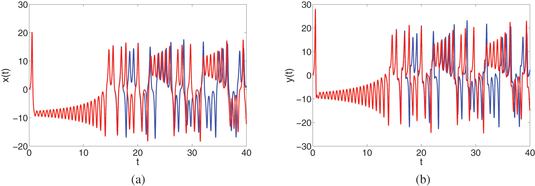
Figure 3: The sensitivity of the state variables in the system (2) towards initial conditions vs. t

6  Conclusion

In the present work, we have derived some theoretical results based on some fixed point theorems due to Banach and Krassnoselskii for the existence and uniqueness of approximate solutions and their computation corresponding to the famous Lorenz nonlinear dynamical system. Sufficient conditions have been developed for the existence and uniqueness of solutions to the proposed model. Also, utilizing U-H and generalized U-H concepts, we have derived a few results for stability under some conditions for the considered system. Further, using a hybrid technique based on the Laplace transform and the Adomian decomposition method, we have also established an algorithm for approximate solutions. Some chaotic behaviors of the Lorenz system have been presented under the given fractional order by using five terms of approximate solution. Also, convergence and sensitivity of the model have been discussed. The proposed method has some features like being easy to implement, no need for prior discretization, and neither depends on auxiliary parameters like the homotopy analysis method. Also, the method is rapidly convergent in many cases. In future, we will investigate the aforesaid Lorenz model under piece-wise equations with fractional order derivative.

Funding Statement: The authors would like to acknowledge the financial support of Taif University Researchers Supporting Project No. (TURSP-2020/162), Taif University, Taif, Saudi Arabia. The authors extends their appreciation to the Deanship of Scientific Research at King Khalid University for funding this work through research groups program under Grant No. R.G.P.1/195/42.

Conflicts of Interest: The authors declare that they have no conflicts of interest to report regarding the present study.

References

1. Wang, J., Li, X. (2016). A uniform method to Ulam-Hyers stability for some linear fractional equations. Mediterranean Journal of Mathematics, 13(2), 625–635. DOI 10.1007/s00009-015-0523-5. [Google Scholar] [CrossRef]
2. Lazarevic, M. P., Spasic, A. M. (2009). Finite-time stability analysis of fractional order time-delay systems: Gronwall’s approach. Mathematical and Computer Modelling, 49(3–4), 475–481. DOI 10.1016/j.mcm.2008.09.011. [Google Scholar] [CrossRef]
3. Garra, R., Orsingher, E., Polito, F. (2018). A note on hadamard fractional differential equations with varying coefficients and their applications in probability. Mathematics, 6(1), 4. DOI 10.3390/math6010004. [Google Scholar] [CrossRef]
4. Caputo, M., Fabrizio, M. (2015). A new definition of fractional derivative without singular kernel. Progress in Fractional Differentiation & Applications, 1(2), 73–85. [Google Scholar]
5. Alqudah, M. A., Abdeljawad, T., Shah, K., Jarad, F., Al-Mdallal, Q. (2020). Existence theory and approximate solution to prey-predator coupled system involving nonsingular kernel type derivative. Advances in Difference Equations, 2020(1), 1–10. DOI 10.1186/s13662-020-02970-w. [Google Scholar] [CrossRef]
6. Sher, M., Shah, K., Feckan, M., Khan, R. A. (2020). Qualitative analysis of multi-terms fractional order delay differential equations via the topological degree theory. Mathematics, 8(2), 218. DOI 10.3390/math8020218. [Google Scholar] [CrossRef]
7. Abdeljawad, T. (2017). Fractional operators with exponential kernels and a lyapunov type inequality. Advances in Difference Equations, 2017(1), 1–11. DOI 10.1186/s13662-017-1285-0. [Google Scholar] [CrossRef]
8. Benchohra, M., Bouriah, S. (2015). Existence and stability results for nonlinear boundary value problem for implicit differential equations of fractional order. Moroccan Journal of Pure and Applied Analysis, 1(1), 1–16. DOI 10.7603/s40956-015-0002-9. [Google Scholar] [CrossRef]
9. Dasbasi, B. (2021). Stability analysis of an incommensurate fractional-order SIR model. Mathematical Modelling and Numerical Simulation with Applications, 1(1), 44–55. [Google Scholar]
10. Akgul, A., Arslan, C., Aricioglu, B. (2019). Design of an interface for random number generators based on integer and fractional order chaotic systems. Chaos Theory and Applications, 1(1), 1–18. [Google Scholar]
11. Korkmaz, N., Saçu, I. E. (2021). An efficient design procedure to implement the fractional-order chaotic jerk systems with the programmable analog platform. Chaos Theory and Applications, 3(2), 59–66. [Google Scholar]
12. Sene, N. (2021). Analysis of a fractional-order chaotic system in the context of the caputo fractional derivative via bifurcation and lyapunov exponents. Journal of King Saud University-Science, 33(1), 101275. DOI 10.1016/j.jksus.2020.101275. [Google Scholar] [CrossRef]
13. Das, S., Pan, I. (2011). Fractional order signal processing: Introductory concepts and applications. Berlin: Springer Science & Business Media. [Google Scholar]
14. Wang, J., Shah, K., Ali, A. (2018). Existence and Hyers-Ulam stability of fractional nonlinear impulsive switched coupled evolution equations. Mathematical Methods in the Applied Sciences, 41(6), 2392–2402. DOI 10.1002/mma.4748. [Google Scholar] [CrossRef]
15. Wang, C. (2019). Stability of some fractional systems and laplace transform. Acta Mathematica Scientia, Series A, 39(1), 49–58. [Google Scholar]
16. Podlubny, I. (1999). Fractional differential equations: Mathematics in science and engineering. New York: Academic Press. [Google Scholar]
17. Poland, D., (1993). Cooperative catalysis and chemical chaos: A chemical model for the lorenz equations. Physica D: Nonlinear Phenomena, 65(1–2), 86–99. DOI 10.1016/0167-2789(93)90006-M. [Google Scholar] [CrossRef]
18. Borisut, P., Kumam, P., Ahmed, I., Sitthithakerngkiet, K. (2019). Nonlinear caputo fractional derivative with nonlocal Riemann-Liouville fractional integral condition via fixed point theorems. Symmetry, 11(6), 829. DOI 10.3390/sym11060829. [Google Scholar] [CrossRef]
19. Kilbas, A. A., Srivastava, H. M., Trujillo, J. J. (2006). Theory and applications of fractional differential equations, vol. 204. Amester Dam: Elsevier. [Google Scholar]
20. Barrio, R., Serrano, S. (2007). A three-parametric study of the lorenz model. Physica D: Nonlinear Phenomena, 229(1), 43–51. DOI 10.1016/j.physd.2007.03.013. [Google Scholar] [CrossRef]
21. Alomari, A. K. (2011). A new analytic solution for fractional chaotic dynamical systems using the differential transform method. Computers & Mathematics with Applications, 61(9), 2528–2534. DOI 10.1016/j.camwa.2011.02.043. [Google Scholar] [CrossRef]
22. Wang, S., Yu, Y. (2012). Application of multistage homotopyperturbation method for the solutions of the chaotic fractional order systems. International Journal of Nonlinear Science, 13(1), 3–14. [Google Scholar]
23. He, S., Sun, K., Banerjee, S. (2016). Dynamical properties and complexity in fractional-order diffusionless lorenz system. The European Physical Journal Plus, 131(8), 1–12. [Google Scholar]
24. Alomari, A. K., Noorani, M. S. M., Nazar, R., Li, C. P. (2010). Homotopy analysis method for solving fractional lorenz system. Communications in Nonlinear Science and Numerical Simulation, 15(7), 1864–1872. DOI 10.1016/j.cnsns.2009.08.005. [Google Scholar] [CrossRef]
25. Rasimi, K., Seferi, Y., Ibraimi, A., Sadiki, F. (2019). Numerical-analytical solution of nonlinear fractional-order lorenz’s system. Applied Mathematical Sciences, 13(13), 595–606. [Google Scholar]
26. Yu, Y., Li, H. X., Wang, S., Yu, J. (2009). Dynamic analysis of a fractional-order lorenz chaotic system. Chaos, Solitons & Fractals, 42(2), 1181–1189. DOI 10.1016/j.chaos.2009.03.016. [Google Scholar] [CrossRef]
27. Toufik, M., Atangana, A. (2017). New numerical approximation of fractional derivative with non-local and non-singular kernel: Application to chaotic models. The European Physical Journal Plus, 132(10), 1–16. [Google Scholar]
28. Algahtani, O. J. J. (2016). Comparing the Atangana-Baleanu and Caputo-Fabrizio derivative with fractional order: Allen Cahn model. Chaos, Solitons & Fractals, 89, 552–559. DOI 10.1016/j.chaos.2016.03.026. [Google Scholar] [CrossRef]
29. Atanackovic, T. M., Pilipovic, S., Zorica, D. (2018). Properties of the caputo-fabrizio fractional derivative and its distributional settings. Fractional Calculus and Applied Analysis, 21(1), 29–44. DOI 10.1515/fca-2018-0003. [Google Scholar] [CrossRef]
30. Ali, F., Saqib, M., Khan, I., Ahmad Sheikh, N. (2016). Application of Caputo-Fabrizio derivatives to MHD free convection flow of generalized walters-B fluid model. The European Physical Journal Plus, 131(10), 1–10. DOI 10.1140/epjp/i2016-16377-x. [Google Scholar] [CrossRef]
31. Gómez, J. F., Torres, L., Escobar, R. F. (2019). Fractional derivatives with mittag-leffler kernel. New York: Springer International Publishing. [Google Scholar]
32. Wang, C. (2021). Hyers-Ulam-Rassias stability of the generalized fractional systems and the
33. Atangana, A., Akgül, A., Owolabi, K. M. (2020). Analysis of fractal fractional differential equations. Alexandria Engineering Journal, 59(3), 1117–1134. [Google Scholar]
34. Haq, F., Shah, K., ur Rahman, G., Shahzad, M. (2018). Numerical solution of fractional order smoking model via laplace adomian decomposition method. Alexandria Engineering Journal, 57(2), 1061–1069. [Google Scholar]
35. Ali, A., Shah, K., Khan, R. A. (2018). Numerical treatment for traveling wave solutions of fractional whitham-broer-kaup equations. Alexandria Engineering Journal, 57(3), 1991–1998. [Google Scholar]
36. Jia, Q. (2007). Hyperchaos generated from the lorenz chaotic system and its control. Physics Letters A, 366(3), 217–222. [Google Scholar]
37. He, J. H. (2000). A coupling method of homotopy technique and perturbation to volterra integro-differential equation. International Journal of Non-Linear Mechanics, 35(1), 37–43. [Google Scholar]
38. Agarwal, P., Jleli, M., Samet, B. (2018). Fixed point theory in metric spaces, recent advances and applications. Singapore: Springer. [Google Scholar]
Cite This Article
Copyright © 2023 The Author(s). Published by Tech Science Press.
This work is licensed under a Creative Commons Attribution 4.0 International License , which permits unrestricted use, distribution, and reproduction in any medium, provided the original work is properly cited.
Downloads
Citation Tools