An Improved Farmland Fertility Algorithm with Hyper-Heuristic Approach for Solving Travelling Salesman Problem

1  Introduction

The TSP is one of the NP-hard problems and has been the subject of numerous investigations. Despite this, none of them has been able to completely address the problem, which is a discrete hybrid optimization problem. Its purpose is to determine the shortest Hamilton route that visits each city precisely once before returning to the starting location, making the short route feasible. Even though this problem has a basic mathematical model and is straightforward to understand, it is challenging to solve. Therefore, it will require more computational time and resources. We cannot solve this problem conclusively because it is NP-hard, and the solutions offered are relative and comparative. Thus, we wish to propose a new method that is more efficient than prior ones. Consider a TSP case with n cities; we can model TSP using the following formula. Assume a distance matrix D = (di, j)n * n is used to hold distances between all pairs of cities, with each entry di, j representing the distance between city i and city j. To define a solution, we can utilize x, a permutation of cities, which means the visiting sequence of cities. TSP’s purpose is to find a solution x (as Eq. (1)) that is as small as possible.

f(x)=∑i=1n−1dxixi+1+dxi,x1(1)

The primary goal of the TSP problem is to identify the shortest Hamiltonian path on a weighted graph [1,2]. Because the computing time for solving large-scale problems is relatively high, various approaches have been given to solve the TSP problem, which is exact and suitable for small and medium optimization tasks. Cutting planes [3], branch and price [4], branch and bound [5], branch and cut [6], and Lagrangian dual [7] are only a few examples of correct approaches. They must discover appropriate (but not necessarily optimal) solutions to these problems in general, which has led to the invention of numerous approximation methods, such as metaheuristic algorithms [8,9]. Multiple metaheuristic algorithms provide advantages such as simplicity and versatility [10,11]. Researchers in [12] proposed many techniques, including hybridization of Simulated Annealing (SA) with Symbiotic Organisms Search (SOS) optimization algorithm to solve the TSP.

The goal is to test this hybrid approach’s convergence and scalability in large and small tasks [13]. For all TSPs in [14], the PSO method was paired with quantum-inspired behavior. TSPLIB instances have been analyzed in three groups of scales using LK for local search in this technique (small, medium, and large scale). A hybrid model, which combines an Ant Colony Optimization (ACO), remove-sharp, local-opt, and genetic algorithm, was proposed to solve the TSP problem [15]. Its purpose is to optimize the search space and present an efficient solution to complex issues by accelerating convergence and positive feedback.

Heuristic crossover and an Expanding Neighbourhood Search (ENS) approach apply honey bees’ mating optimization to solve TSP [16]. A heuristic crossover extracts standard and unique traits from parents and uses ENS to combine numerous local searches. Furthermore, this strategy has been utilized to solve TSP using a master-slave system with several colonies [17]. This approach has been integrated with 3-Opt to boost performance in a distributed computing environment where these colonies communicate regularly. Each colony runs this algorithm independently, and the results are shared with the other territories. This approach has been tested in 21 different scenarios. This algorithm has also been merged with LK local search. It received a score of 64 TSPLIB. A hyper-heuristic is a method for selecting or developing an automated set of heuristics [18].

Selection hyper-heuristics and generation hyper-heuristics are the two types of hyper-heuristics [19–25]. It is categorized into two kinds: perturbative and constructive. The constructive hyper-heuristic eventually generates a complete solution based on the nature of heuristics [26,27]. The perturbative hyper-heuristic improves the resolution by continually applying disruptive procedures. Low-level heuristics (LLHs) are developed or selected by hyper-heuristics. The evaluation function(s) and issue representation are two general layers of an LLH. To manage LLH selection to produce new solutions and make judgments in adopting new solutions, a collection of LLHs and the HLH are used [28]. The diversity component chooses the LLHs. As a result, it’s critical to balance diversity and intensity [29]. We should employ an LLH that performs well at one level of repetition to enhance the answer in future phases. Also, even if an LLH performs poorly at one step of repetition, we should not completely abandon its usage.

In this paper, we have improved the FFA [30] to use it to solve the TSP problem. It measures the quality of every part of their farmland at their visit and improves soil quality by using fertilizers and organic matter. Lower-quality parts of the land receive materials and the changes in this part of the farmland are more significant than in other regions. A memory alongside each segment has the best possible solution called local memory. Moreover, the memory with the best quality and resolution in all sections is global. Finally, they combine each section’s soils with the soil and solution of global memory & local memory to obtain high-quality soil and solution. This paper has presented and improved this algorithm based on the previous paragraphs’ methods, and then we have compared the simulation results with this method and other procedures. The findings reveal that our suggested technique is superior to other methods, and LLH selection is based on the MCF selection function and merged with the FFA. In particular, MCF has been used in soil improvement for the other two areas. MCF has been used to control its weights in intensification and diversification during the search process’s various steps. Moreover, the proposed algorithm has been integrated with LK local search to improve performance [31]. The proposed algorithm was tested on the datasets available in TSPLIB [32].

The following are the paper’s most important advancements and contributions:

⮚   The FFA algorithm has been presented for solving hybrid discrete optimization problems, and to interrupt this algorithm, we used the ten neighborhood search operators.

⮚   To increase the FFA algorithm’s performance, and since the FFA algorithm was designed to solve an ongoing issue, the section of soil composition in permutation problems may be time-consuming and difficult. As a result, we have selected the best answer in each part and then done operations to enhance the solution to concentrate more on the chosen solutions.

⮚   A hyper-heuristic approach based on MCF was applied intelligently and automatically, choosing neighborhood search operators.

⮚   A local search strategy known as LK was applied to boost the performance of the proposed algorithm.

⮚   Three improved versions of the FFA algorithm (MCF-FFA and (4 LLH) MCF-FFA and Random-FFA) have been presented and evaluated. Finally, MCF-FFA outperformed the other two approaches. Therefore, it was named MCF-FFA.

⮚   With 71 cases and three criteria, the TSP evaluated the proposed algorithm. The new approach was compared to 11 previously reported models, indicating acceptable.

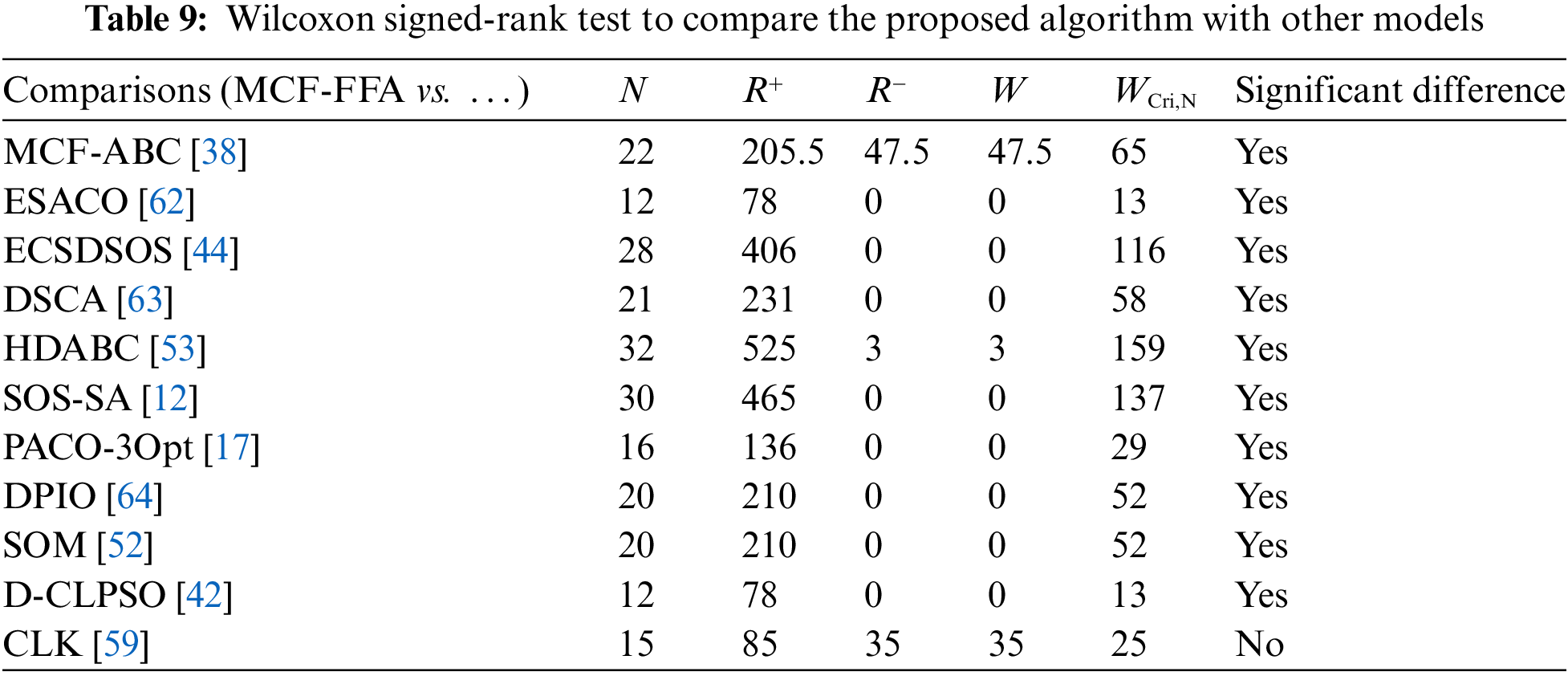
⮚   The Wilcoxon signed-rank test compared the proposed algorithm to other models.

We ordered the framework of this paper as follows: we reviewed the related works in Section 2, explained the basic concepts in Section 3, and outlined the proposed algorithm in Section 4. In Section 5, proposed algorithms were compared and then evaluated. Finally, we concluded in Section 6.

2  Related Works

Over the years, several researchers have developed several approaches and algorithms for solving the TSP issue. It is difficult to propose a specific algorithm for the TSP problem since it is an NP-Hard problem. As a result, academics have constantly attempted to find ways to make prior approaches more efficient. We have mentioned some earlier works proposed to solve the TSP problem here. Finally, we have presented and compared the algorithm with some of these methods and algorithms.

The ACO algorithm and the Max-Min approach [33] have been integrated. It is paired with the Max-Min approach, which uses four vertices and three lines of inequality to find the best Hamiltonian circuit. In [34], they utilize a wolf colony search algorithm to solve the TSP problem that uses a siege strategy to achieve the following goals: improvement of the mining ability, reduction of the siege range, and acceleration of the convergence time. Also, the immune-inspired self-organizing neural network has been used to solve the TSP problem [35]. By comparing it to other artificial neural network algorithms, they concluded that this method demands a more significant time for convergence in many cases. Still, the quality of the solutions improves dramatically. The Kernel function has added a threshold value to update antibodies, and the winners’ stabilization mechanism has been used to improve the method. A discrete firework algorithm has been presented to solve the TSP problem [36] that uses two local Edge-exchange heuristic algorithms (namely: 2-Opt and 3-Opt) to perform the essential explosion operation of the firework algorithm. And in [37], a discrete tree-seed algorithm has been used to solve the TSP problem, which uses three swap, shift, and symmetry operators to generate seeds.

Furthermore, the 2-Opt approach enhanced the solutions and tested many TSP problems. The discrete ABC algorithm has been improved using a hyper-heuristic method called MCF [38]. MCF can intelligently and automatically select each of the LLHs algorithms during the algorithm’s execution. Generally, 10 LLHs have been used, such as RI, RRIS, RIS, RS, RRSS, RRS, RSS, Random Shuffle Swap of Subsequence (RSSS), Random Shuffle Insertion of Subsequences (RSIS)), and Shuffle Subsequence (SS). The proposed algorithm is also integrated with LK and evaluated with other models using 64 TSP Instances, which this algorithm obtains good results.

In [39], a cuckoo search algorithm with a random-key encoding method solved the TSP problem, transferring the variables from continuous to discrete space. Then, this algorithm was integrated with the 2-Opt move, and TSP Instances in the TSPLIB library were used to investigate this algorithm’s performance. A new method has also been presented for solving the TSP problem using a bacterial foraging optimization algorithm [40]. The critical step in the proposed work is the calculation of chemotaxis, in which bacteria move around the prospect of looking for food to reach high-nutrient areas.

The ABC algorithm for solving TSP has been updated and presented new ways. One of these variants is the hybridization ABC (CABC) algorithm, a hybrid version of standard ABC. Another model is the Quick CABC Algorithm, an enhanced version of the CABC Algorithm (QCABC) [41]. 15 TSP benchmarks were used to compare the performance of these two versions of the ABC method. Eight different factors were used to compare the performance of these two methods (GA variants). Moreover, several analyses have been performed on setting the limit and CPU time parameters of the QCABC and CABC algorithms.

In addition, a discrete comprehensive learning Particle Swarm Optimization (PSO) algorithm with Metropolis acceptance criteria was introduced to address the TSP problem [42]. The Anglerfish algorithm was proposed to solve the TSP problem in [43]. With the Randomized Incremental Construction approach, this algorithm executes search operations randomly depending on the beginning population. It facilitates a random sample search without the need for a time-consuming technique.

A Discrete SOS (DSOS) algorithm was introduced by employing excellent coefficients and a self-escape strategy [44] for solving the TSP problem. It does not get stuck in local minima because of the self-escape method. Shorter edges are chosen using the excellence coefficients to generate better local pathways. Finally, the TSP problem has been solved using the approaches mentioned below. Discrete Cuckoo Search [45], Discrete SOS [46], ACO [47], Efficient hybrid algorithm [48], parallel ACO algorithm [49], Improved genetic algorithms [50], Hybrid Genetic Algorithm [51], Massively Parallel Neural Network [52], Hybrid Discrete ABC with Threshold Acceptance Criterion [53], pre-processing reduction method [54], Spider Monkey Optimization [55], etc.

3  Fundamental Research

3.1 Farmland Fertility Optimization Algorithm

FFA is a metaheuristic method based on agricultural fertility described in [30]. Farmers split their farms into sections based on soil quality, enhancing the soil quality in each region by adding particular materials. Due to their quality, these materials may have different types, and farmers add them to the soil at each visit; this quality is stored in memory next to each section. As a result, the best material is sent to the worst area of the farmland. In this approach, the best quality in each segment is termed local memory, and the best soil quality in all portions is called global memory. In other words, local memory saves the best solution in each segment, but global memory keeps the best solution across all search areas. These memories are employed to enhance the solutions in the ensuing optimization process. As a result, the component with the lowest quality is coupled with one of the global memory solutions. All the solutions in the search space are integrated with the solutions from the other parts. Following this step, each section’s answers are linked to one of the best global or local memory solutions. There are six general steps in the algorithm. The following is the first step.

Step 1: Initializing parameters used in the algorithm

The total population is obtained using Eq. (2) in the FFA algorithm.

N=k∗n(2)

In Eq. (2), N is the total population in the problem space, and k represents the sections. Moreover, the number of solutions in each section is described by n., and k must be an integer greater than zero. Of course, k can be a number between 1 and N. However, the authors have stated [30] that if this value is initialized equal to 1 or greater than 8, it decreases the algorithm’s performance. Therefore, this number must be 2 ≤ k ≤ 8, and these results are obtained by trial and error. Eq. (3) is used to generate the search space randomly.

xij=Li+rand(0,1)×(Uj−Lj)(3)

In Eq. (3), Ljis the lower bound and Uj is the upper bound of the variable x, and rand is by a function generates random integers between 0 and 1, and j = [1, …, D] represents the dimensions of x, and i equals the total population [1, …, N].

Step 2: Determination of soil quality in each part of the farm

After generating the initial population and evaluating each solution’s fitness, each section’s quality is assessed using Eqs. (4) and (5).

Sectionss=x(aj),j={1,2,…,4},a=n∗(s−1):n∗s,s={1,2,…,k}(4)

In Eq. (4), x represents all solutions in the search space, s the number of parts, and j = [1, …, D] the dimension of the variable x.

FitSectionss=Mean(allFit(xji)inSections),i={1,2,…,n},s={1,2,…,k}(5)

In Eq. (5), for each section of farmland, Fit_Section display the worth and quality of the solutions.

Step 3: Updating the memory

Some of the best solutions in each section are stored in local memory. In all areas of global memory, the optimal solution is stored. Eq. (6) provides the number of best local memories, whereas Eq. (7) provides the best global memories.

Mlocal=round(t∗n)0.1<t<1(6)

MGlobal=round(t∗N)0.1<t<1(7)

Step 4: Alteration of the soil quality

The worst section is paired with one of the global memory solutions to produce the most significant improvement at this step. It is expressed by Eqs. (8) and (9).

h=α∗rand(−1.1)(8)

Xnew=h∗(Xij−XMGlobal)+Xij(9)

where, α is a parameter between 0 and 1. h is a decimal number obtained by Eq. (8) and Xnew is the new solution. XMGlobal is a random solution available in global memory, and Xij is the selected solution in the worst section. After making changes to the explanations of the worst section, the other sections’ solutions are combined with the complete search space solutions using Eqs. (10) and (11).

h=β∗rand(0.1)(10)

Xnew=h∗(Xij−Xuj)+Xij(11)

where, β is a parameter between 0 and 1. Xuj is a random solution in the search space. Xij is a selective solution among all sections, except for the worst section. h is a decimal and Xnew is a new solution.

Step 5: Integrating soil

All solutions are integrated with one of the best solutions in the local or global memory, as illustrated by Eq. (12).

H={Xnew=Xij+ω1∗(Xij−BestGlobal(b)).Q>randXnew=Xij+rand(0.1)∗(Xij−BestLocal(b)).else(12)

In Eq. (12), the parameter Q determines which of the solutions should be combined with BestGlobal. This parameter must be initialized between 0 and 1 before the start of the algorithm. The value of ω1 parameter must be an integer and must be set before the algorithm begins. This parameter’s value rapidly lowers with each iteration of the method, as seen in Eq. (13).

ω1=ω1∗Rv.0<Rv<1(13)

Step 6: Termination conditions

The algorithm’s termination criteria are reviewed at the end of each step of the algorithm iteration. The algorithm ends if the constraints are satisfied. Otherwise, the algorithm will keep working until the termination constraints are satisfied.

3.2 Neighborhood Operators

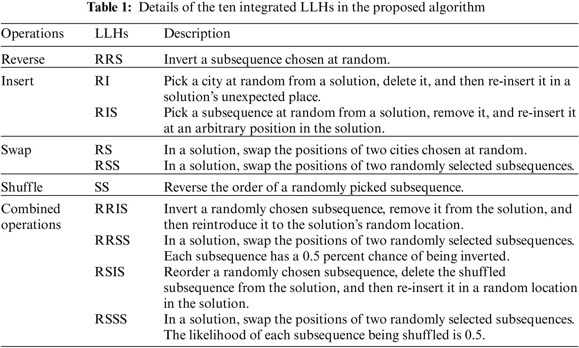
These operators are applied to get the best results. These operators are also classified into two categories: point-to-point and subsequence. One city is chosen to change in point-to-point operators, but many cities are selected to vary in sequence operators. Point-to-point operators include RS and RI; subsequence operators include RSS, RIS, RRS, RRIS, SS, RSIS, RSSS, and RRSS. The proposed algorithm incorporates these ten operators as 10 LLHs composed of four primary operations-insert, shuffle, swap, and reverse. RRS performs specifically a function to change the subsequence. RI and RIS perform an insert operation. The swap and shuffle operations are performed by RS and RSS, whereas SS. RRIS performs the shuffle operation; RRSS, RSIS, and RSSS are four of the ten LLHs that are a hybridization of two operators. Note that RRS, RIS, RSS, SS, and the four LLHs with combined operations consider a subsequence of a TSP solution in size range [2: dim], where dim represents the TSP dimension. These operators have been listed in Table 1.

3.3 Modified Choice Function

A version of the choice function is MCF heuristic selection. Within the heuristic search process, it promotes intensity above diversification. A choice-function-based hyper-heuristic with a score-based method is provided in [56]. Each LLH’s rating model is evaluated based on the LLH’s prior performance. Each LLH’s score is made up of three different criteria: f1,f2 & f3. In this model, the criterion of first measurement is f1 and the recent performance of each LLH is calculated by Eq. (14).

f1(hj)=∑nαn−1In(hj)Tn(hj)(14)

In Eq. (14), α is a parameter between zero and one that prioritizes recent performance, hj is the same LLHj, In(hj) shows the nth use of hj displays the value of the difference between the current and new solutions. Tn(hj) expresses the amount of time spent by nth use of hj to propose a new solution.

f2(hk,hj)=∑nβn−1In(hk,hj)Tn(hk,hj)(15)

In Eq. (15), f2 shows the dependence between a successive pair of LLHs. In(hk,hj) shows the value of the difference between the new solution using nth successive use of hk and hj and the current solution. Tn(hk,hj) shows the amount of time spent by nth sequential use of hk and hj to propose a new solution, β is a parameter between zero and one that prioritizes recent performance. Two criteria, f1 and f2, increase the selection of LLHs with high performance are components of intensification in the selection function. The third criterion, f3, records the time spent for the last implementation of a particular LLH (Eq. (16)).

f3(hj)=τ(hj)(16)

In Eq. (16), τ(hj) indicates the time spent for the last execution of hj (in seconds). Note that f3 performs its work as a component of diversification in the selection function. It prioritizes those LLHs that have not been used for a long time. The score of each LLH is calculated using the sum of the weights of three criteria (f1,f2&f3), as in Eq. (17) is shown.

F(hj)=αf1(hj)+βf2(hk,hj)+δf3(hj)(17)

In Eq. (17), the weight of the criteria is as follows (f1,f2&f3) represented by the α, β, and δ parameters. These parameters are constant values in the initial model. In [57], they have proposed an improved version of the hyper-heuristic to increase performance. In this version, if an LLH makes the solution better, the values of parameters β and α increase the new solution’s improvement rate compared to the previous solution. However, if the selected LLH does not improve the solution, the parameters α and β are reduced due to the difference between the new solution’s costs and the previous solution. Therefore, it can earn many rewards. Moreover, improving solutions in subsequent optimization phases may be reduced due to the convergence of one of the optimal solutions. As a result, much fewer rewards will be gained. Improvements in the subsequent optimization steps are far more essential than improvements in earlier ones. Therefore, the reward-penalty mechanism is not the correct mechanism. In addition to these limitations, the LLH selection mechanism must be randomly performed if solutions are not improved after several repetitions. Because the values of parameters α and β are reduced due to the reward-penalty mechanism. Also, the criterion f3 that is, a diversification component prevails over other criteria. Due to the limitations stated in [57] an improved version of the selection function. In this selection function version, parameters α and β are combined into a single parameter called μ. Finally, Eq. (18) computes each LLH’s score.

Ft(hj)=μt[f1(hj)+f2(hk,hj)]+δf3(hj)(18)

The intensification component is prioritized if an LLH improves the solution and the parameter approaches its maximum static value around 1. The parameter δ is reduced to a minimum static value close to zero at the exact moment. If LLH does not improve the solution, the μ parameter will be penalized linearly and lower (0.01). This mechanism causes the parameter δ to grow with uniform and low speed. The parameters μ and δ are calculated using Eqs. (19) and (20). Eq. (19) shows the difference between its cost and the previous solution’s cost.

μt(hj)={0.99,d>0max[0.01,μt−1(hj)−0.01],d≤0(19)

δt(hj)=1−μt(hj)(20)

The proposed algorithm uses MCF to select the best automatic LLHs during optimization implementation to increase the proposed algorithm’s performance and efficiency.

3.4 Local-Search-Based Strategies (LK Local Search)

Local search solves many hybrid optimization problems because it increases the ability to solve them. Researchers have proposed various types of local search such as Opt-2, Opt-3, and local search such as LK. Local search can find optimal solutions; therefore, local search capability is limited to intensification. A method increases the probability of finding a global optimum that restarts the search after exploiting a particular search area. This type of local search that uses a re-search mechanism is called the Multi-start Local Search (MSLS) [58]. In MSLS, it is only possible to search for different primary solutions. Finally, we can obtain a set of locally optimal solutions in a globally optimal solution or find a solution close to the global optimum to collect locally optimal solutions. In [59,60], Chained LK (CLK) heuristic has used the ILS mechanism to solve the TSP problem. It is followed in CLK by a double-bridge motion to exchange the four arcs of the solution with the other four arcs, and this operation is done repeatedly on the solution. According to the importance of the balance of exploration and exploitation and the performance improvement in combining metaheuristic and local search algorithms, the proposed MCF-FFA model has been integrated with LK local search. A local search is carried out after each Neighborhood operator, performed on the solutions in bad and other parts before applying the acceptance condition. Due to local search use in the proposed algorithm, this model is very similar to the ILS and MSLS models. Based on the previous explanations, it has many similarities to the ILS and MSLS models.

4  Proposed Algorithm

This paper has improved FFA and examined the results of the TSP problem. First, because the FFA algorithm has been presented to solve the ongoing problem, and our case study is to find the solution for discrete optimization problems such as TSP, this algorithm requires modifications and adaptations.

In the proposed algorithm, considering that the problem space has changed from continuous to discrete, the constant mechanisms of the FFA algorithm do not have the necessary efficiency in searching in the discrete area. Therefore, neighborhood search operators have been used to modify and search the created tours. Each neighbouring operator has a unique feature and applies different changes in each tour. These behaviors make each operator perform better in various stages of the search operation, and selecting the operator at the right time can result in an impressive performance. According to our explanations, the Modified Choice Function (MCF) has been used for the intelligent selection of neighborhood search operators. MCF is selected after using and applying changes from neighborhood search operators, which applies rewards or penalties to each operator based on the cost obtained. This approach is based on three general criteria. But this approach can only help solve problems of medium dimensions. To solve problems with large sizes, after each selection of neighborhood search, LK local search is called and performs search and optimization operations on tour. The above procedure creates an ILS and MSLS model.

Some things need to be changed to adapt this algorithm because it is designed to solve ongoing issues. The following cases can be described:

•   We exchange Eq. (3) with a random permutation in the FFA algorithm. The solutions are divided into the number of segments determined by the parameter K. Then, the cost of each solution and each component is measured. Eventually, the section that costs more than other parts is selected as the worst section.

•    We replace Eqs. (8)–(11) with neighborhood search (i.e., LLHs) to improve solutions in the process of soil improvement and search in a discrete optimization environment. These LLHs are automatically and intelligently selected to solve the problem at every step of MCF’s algorithm implementation. One of these LLHs has been listed in Table 1, and finally, they improve the solutions. In the next step, any updated solution using MCF is improved using local search, and finally, the selected LLH for improvement is updated using Eq. (18) related to MCF. All these steps are performed on all solutions in the worst and others.

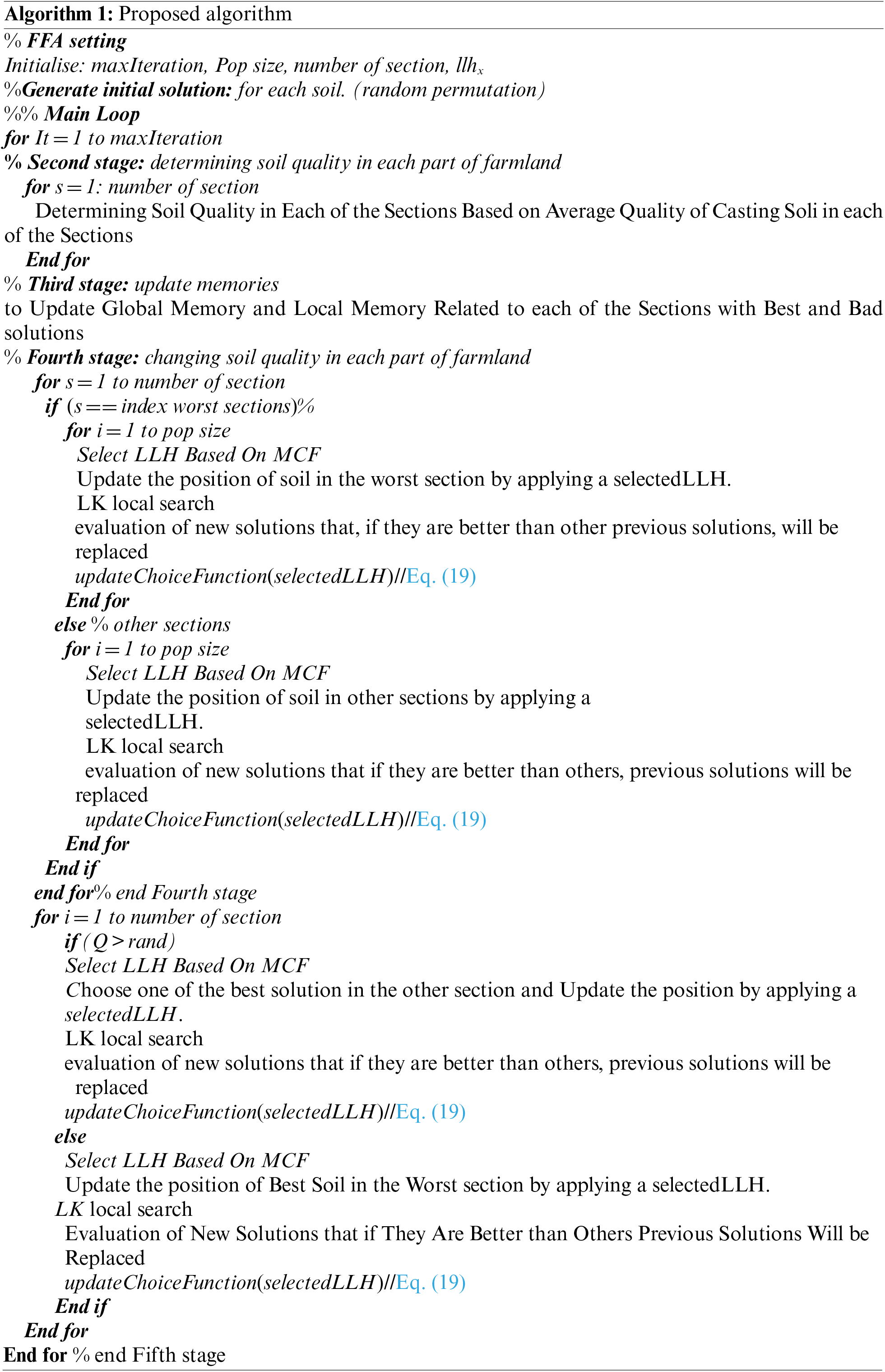
•    The FFA algorithm’s soil composition section is replaced by another better method to solve the TSP problem. In this section’s model, the best solutions in the worst part of the best solutions in the other parts are that these parameters determine the number of parts of the search space and are updated again according to the number of parameters K using MCF improved by local search. The parameter Q value determines the best solution for the wrong parts in each iteration, between 0 and 1. This parameter must be initialized before the optimization operations. The best global solution is improved using this mechanism. The best global solution is one of the best solutions in one of the sections. This section in the algorithm focuses more on the selected solutions in the search space to improve the optimization operation. Our proposed algorithm is described as pseudo-code in Algorithm 1 and the flowchart in Fig. 1.

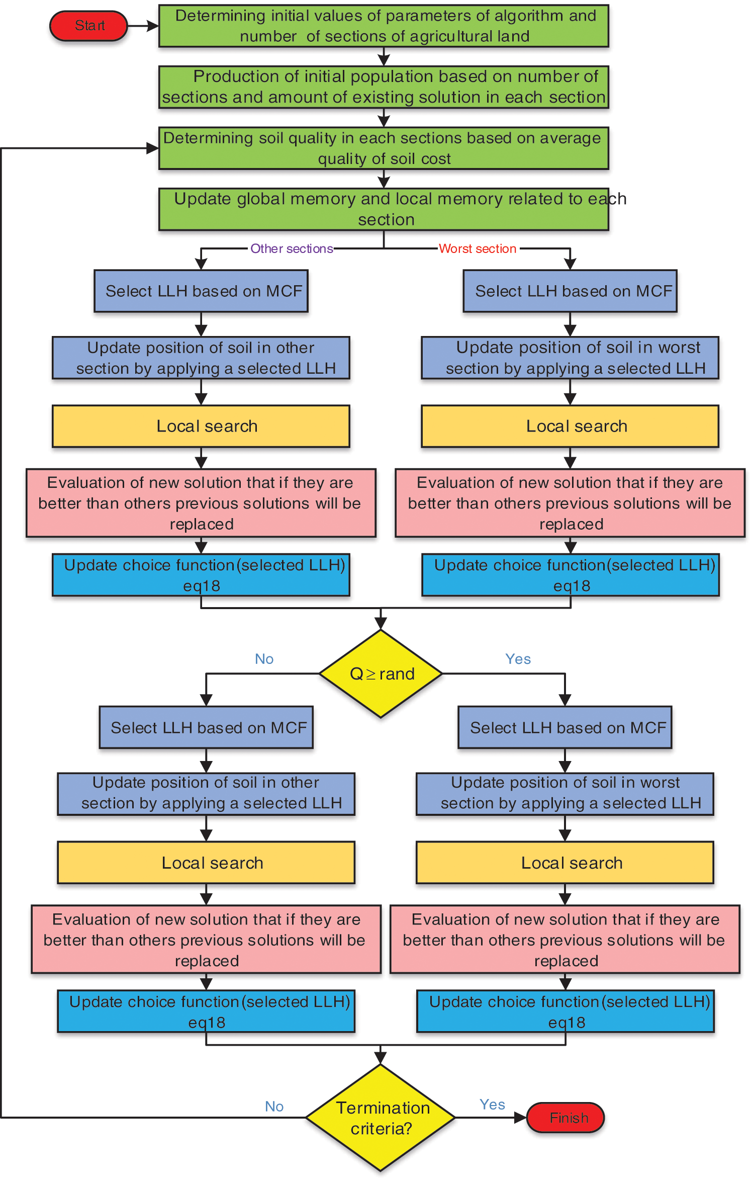
Figure 1: Flowchart of proposed algorithm

5  Result and Discussion

The experimental setting, comparison studies, and experimental results are presented in this section.

5.1 Experimental Settings

A computer with an Intel Core i7-7700k processor 4.50 GHz (CPU) and 16 GB RAM has been used to test the proposed algorithm. It is implemented using the C programming language, and the Concorde [59] is used to implement the LK local search in the proposed algorithm. Seventy-one instances from the TSPLIB [32] with dimensions of 100 to 85,900 cities were used to evaluate the proposed algorithm’s performance. The number of instance names represents the number of cities in an instance. For example, the number of cities equals 100 in the instance kroA100. Two criteria, such as percentage deviation from optimal solution and computational time, were used to obtain the best tour (measured in seconds) to evaluate the performance of the proposed algorithm.

Each of the TSP instances has been investigated for 30 iterations. It was placed the best tour per implementation in the set X = {c1, c2, …, c30} and the computational time to obtain the best tour was placed in another set called T = {t1, t2, …, t30}, where X is the set of best tours, and T is the set of computational time to obtain the best tours, and finally, an average is obtained for these two sets, which µT is used to represent the average of set T. Average represents the mean of the set X. Finally, Eq. (21) is used to describe the percentage deviations of the average solution (PDav) (%). In this equation, BKS is the optimal tour length.

PDav(%)=Average−BKSBKS×100(21)

5.2 Parameter Tuning

In the proposed algorithm, two main POP and K-Value parameters must be adjusted to obtain optimal performance before starting optimization. POP is the population, and K-Value is the number of segments. All the instances are grouped into four categories in terms of their dimensions: Instances with dimensions [1: 500] in category X and instances with dimensions [501: 1000] in category Y, and instances with dimensions [1001: 10000] in category Z and instances with dimensions larger than 10000 in category E. Then an instance is selected as representative of each class. Instances gr202, gr666, rl5915, and rl11849 are chosen to represent the X, Y, Z, and E categories, respectively. Finally, we apply settings related to representatives for all other instances about the best performance results. A decrease in repeats occurs with the increasing population to make a fair comparison. For example, repetition terminates testing the population (10 × 400). Moreover, the replay ends for testing the population size (20 × 200). Table 2 shows the results of different settings for parameters.

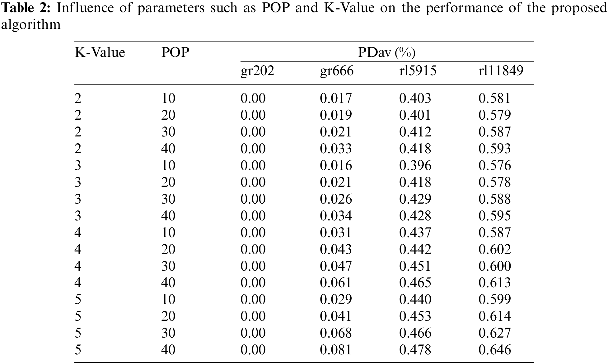
The proposed algorithm in the instance gr202 achieved the optimum for all possible situations in setting the parameters. However, the proposed algorithm’s best performance occurs with POP = 10 and K-Value = 3 in gr666, rl5915, and rl11849. Hence, POP values = ten and K = 3 are considered for solving the other instances.

5.3 Experimental Results

To investigate the performance of LLHs and the effect of integrating LLHs with MCF in this section, three modes of the proposed algorithm are presented below: Random selection of LLHs and integration of the four main LLHs (SS, PRS, RIS, and SS) with MCF, and integration of all LLHs with MCF have been compared to each other. Also, this comparison is performed to evaluate MCF’s performance when integrated with the FFA. Termination condition (400 iterations) is considered for all three modes (MCF-FFA, (LLH4) MCF-FFA and Random-FFA). In Table 3, to evaluate the performance of these three algorithms, we show the average tour length, PDav, and average computational time to obtain the best solution (μ_T).

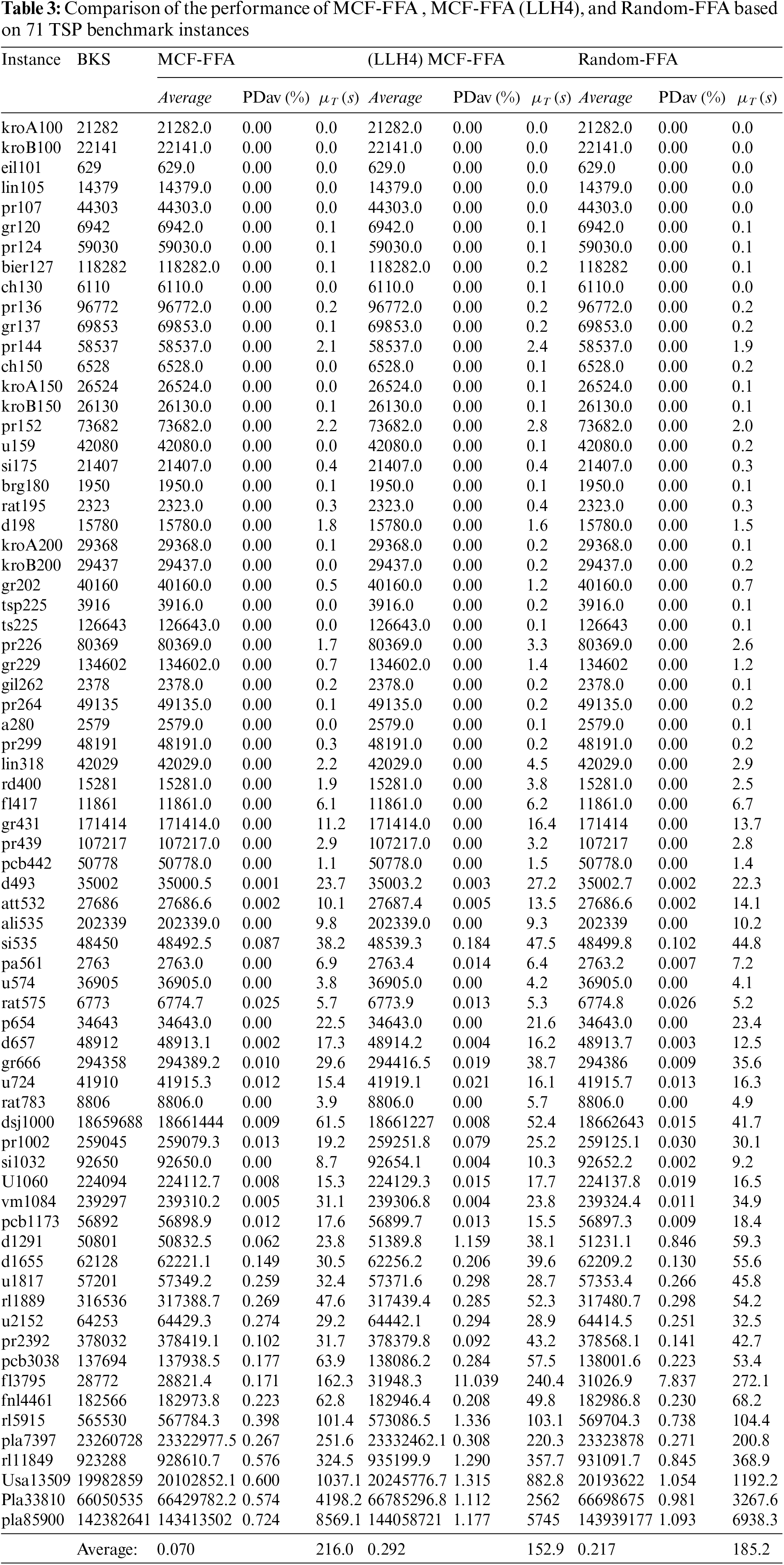
According to Table 3, MCF-FFA has the best performance in finding the best tour. MCF-FFA achieved an average of 0.070 PDav (%), while (LLH4) MCF-FFA and Random-FFA models obtained scores equal to 0.292 and 0.217, respectively, performed worse than the MCF-FFA. The MCF-FFA model solved 44 of 71 instances in 30 iterations. Moreover, in most cases, the model MCF-FFA had a better performance than other models. Of course, in some cases, the two models (LLH4), MCF-FFA and Random-FFA, performed better than others, some of which are shown in Fig. 2.

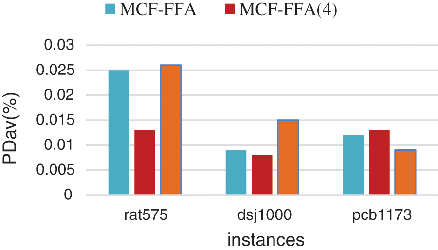
Figure 2: Exhibition of better performance of the two models (LLH4), MCF-FFA and Random-FFA

The most notable instance performed convergence analysis in a TSPLIB (pla85900). The best-so-far was calculated using Eq. (21), and its value in each iteration of three modes (Random-FFA and MCF-FFA and (LLH4) MCF-FFA) has been shown in Fig. 3. (LLH4) MCF-FFA has a fast convergence in the analysis of this chart. However, after a few iterations, it falls into the trap of local optima, but the MCF-FFA and Random-FFA modes are more capable of escaping local optimality. Finally, MCF-FFA has more potential to improve the solution.

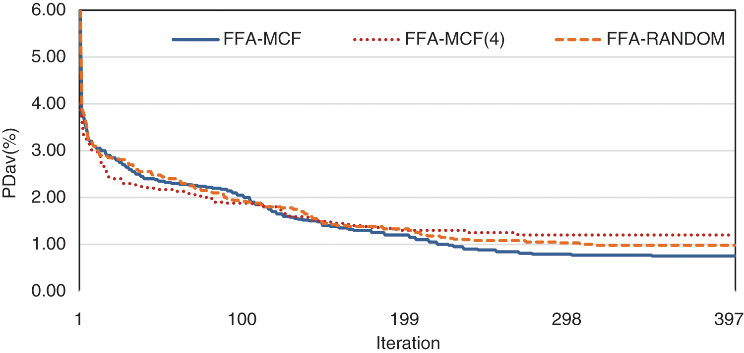
Figure 3: Convergence graph of MCF-FFA and (LLH4) MCF-FFA and random-FFA in solving pla85900

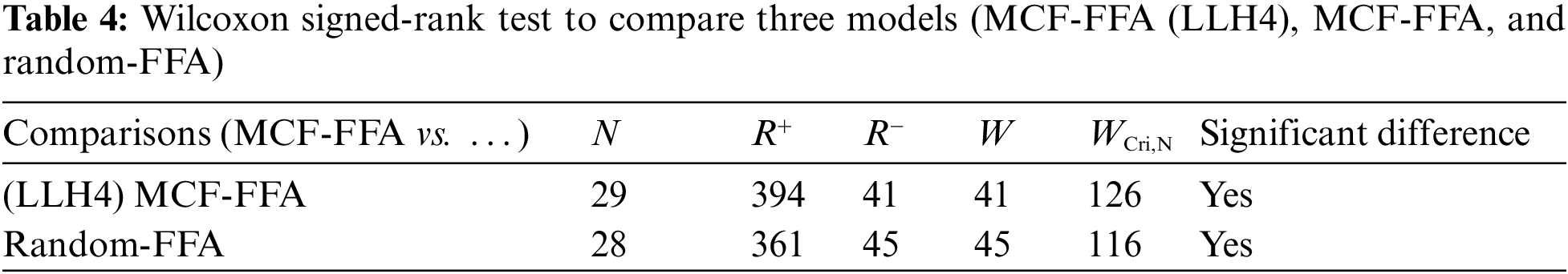
Wilcoxon signed-rank test [61] with 95% confidence interval was used for statistical comparison of the performance of three models (MCF-FFA, (LLH4) MCF-FFA, and Random-FFA). Wilcoxon signed-rank test has used the difference between the value of PDav (%) in two algorithms for comparison and ranking. Instances with similar values in the two algorithms are not used, regardless of similar cases. N denotes the number of sufficient cases, and R+ represents the scores for the cases with the best performance in the proposed algorithm. Whereas R− represents the sum of scores for the instances that the proposed algorithm performs worse than the comparative algorithm, and the value of W is compared with a critical value WCri,N in the Wilcoxon signed-rank test. If  W≤WCri,N, it indicates a significant difference in the performance of the two algorithms. But if W>WCri,N then there is no significant difference in the performance of the two algorithms. Table 4 presents the Wilcoxon signed-rank test for comparison of three models (MCF-FFA, (LLH4), MCF-FFA and Random-FFA) and the results of the Table show the remarkable performance of the MCF-FFA model.

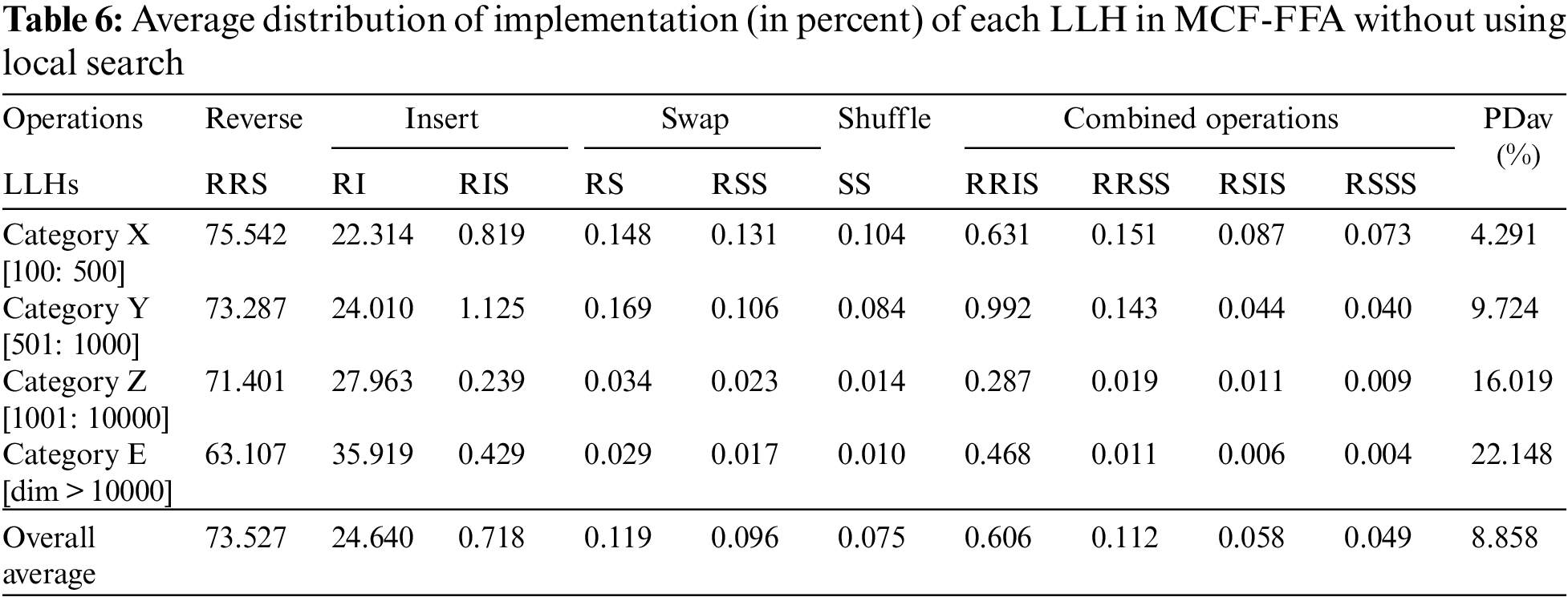
For further evaluation and investigation of the MCF-FFA model, the average distribution of the implementation of each LLH selected by the MCF is recorded in each model’s performance. The 71 TSP instances used to evaluate these are classified into four categories according to their dimensions. Table 5 shows the average distribution of each LLH implementation by MCF when the cases are solved in each class.

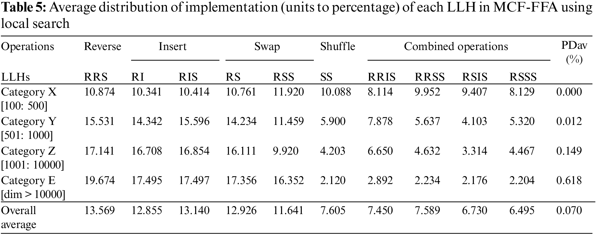
According to the results shown in Table 5, LH (RSS) is selected by MCF over other LLHs in Category X, and MCF prefers LLH (RIS) in comparison with other LLHs in Category Y. Moreover, LLH (RRS) is chosen by MCF in contrast with other LLHs in Category Z. Finally, MCF selects LLH (RRS) in comparison with other LLHs in Category E. In the proposed algorithm, LLHs (such as RRS, RI, RIS, RS, and RSS) are frequently selected by MCF for obtaining good scores from the criteria f1, f2. Because these LLHs create more improvements than other LLHs in a shorter computational time. If the control mechanism in the MCF causes the parameter δ to obtain more value and grow faster in the event of lousy movement, in this case, the diversification component f3 will be prioritized, and LLHs will most likely be selected that were not previously selected. This section has tested the proposed algorithm for further investigation without using LK local search. The results are shown in Table 6 indicate that if the LK local search is deleted, the MCF will select LLHs (RI and RRS) more than other LLHs.

5.4 Competitiveness MCF-FFA

In this subsection, we have compared the MCF-FFA model’s performance with other models. Due to the comparative models’ lack of sources, the published articles’ results were directly extracted and compared. The PDav (%) was used for comparison. In total, ten different models were used for this comparison. Finally, the proposed algorithm has been compared with CLK to evaluate the performance. The selected models for comparison include ESACO [62], written by C++ programming language and executed using an Intel CPU 2.0 GHz processor and 1.0G RAM. These models end with tenants and 300 reps. The SOS-SA model [12] was programmed using Matlab R2014b and run on a computer with a 2.83 GHz CPU Desktop with 2 GB of RAM. MCF-ABC [38] model has been written in C programming language and runs on a system with an Intel i7-3930K 3.20 GHz processor and 15.6 GB of memory. The pop-Size parameter is set to 10, the limit parameter is set to 200, and these parameters are terminated in 1000 iterations. The ECSDSOS model [44] has been implemented using a computer with Intel (R) Core (TM) CPU 2.6 GHz CPU and 4G RAM, and the size of the ecosystem equals 50, and it is terminated in 1,000 reps. The HDABC model [53] is written using Java programming language and is implemented on a computer with Intel Core i7-5600 2.60 GHz CPU and 8 GB RAM and is completed in 500 iterations. The SOM model [52] is implemented on the GPU using the CUDA platform and 1280 MBytes of memory. The PACO-3Opt [17] is written by Java programming language and is implemented on PC with Pentium i5 3.10 GHz processor, and 2 GB RAM and migration interval is set to 5, finished in 1000 iterations. The D-CLPSO [42] is finished in 1000 iterations, and the length of the temperature list and the swarm size are 140 and 20, respectively. The DSCA model [63] has been coded using MATLAB R2014a and implemented using a the computer with a CORE i3 CPU with 2.27 GHz.

Moreover, the population has been considered equal to 15, and the number of generations equals 200. Java programming language is used for coding the DPIO model [64] and is implemented on a computer with Intel Core i5-3470 CPU, with 3.2 GHz and a RAM of 4 GB, and is finished in 1000 iterations. The source of CLK [59] model code available in the Concorde TSP solver software is used to compare the proposed algorithm with CLK. Instances Z and E were used for comparison. CLK is a single solution-based model, and the number population is equal to 1 in this model; a pre-determined number of repetitions are equivalent to 10,000. Default settings in Concorde are maintained for execution, which are: initialization method (i.e., Quick-Boruvka), choice of the kick (i.e., 50-step random-walk kick) and the level of backtracking (i.e., (4, 3, 3, 2)-breadth).

Table 7 has compared the proposed algorithm’s performance with the other models. The proposed algorithm has shown the best performance compared to the different models and has been able to find the optimal tour in most cases. HDABC and MCF-ABC performed better than the proposed algorithm in some instances. MCF-ABC had similar performance in small-scale cases and was able to find optimal tours, and in some cases with different scales, it was able to find better tours than the proposed algorithm. Because the MCF-ABC model employs a strategy similar to the proposed algorithm, the HDABC model only performs well in small-scale instances. To further evaluate the proposed algorithm, a comparison with CLK [59] has been made in Table 8.

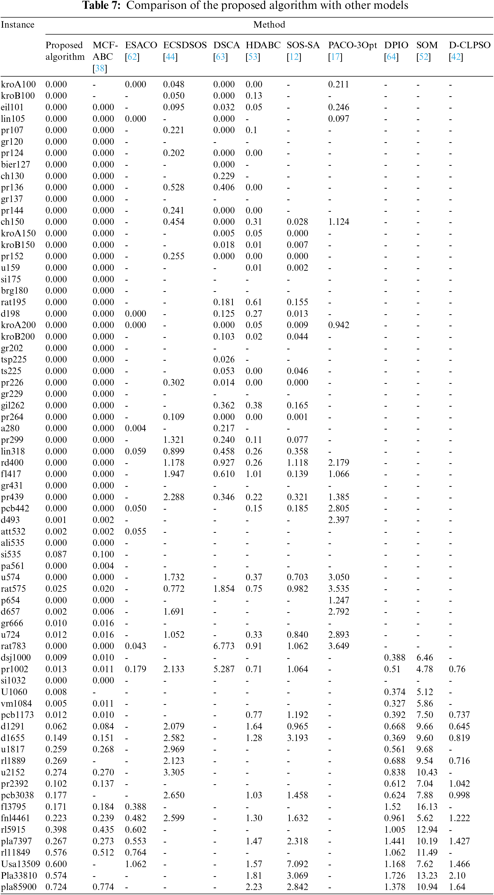
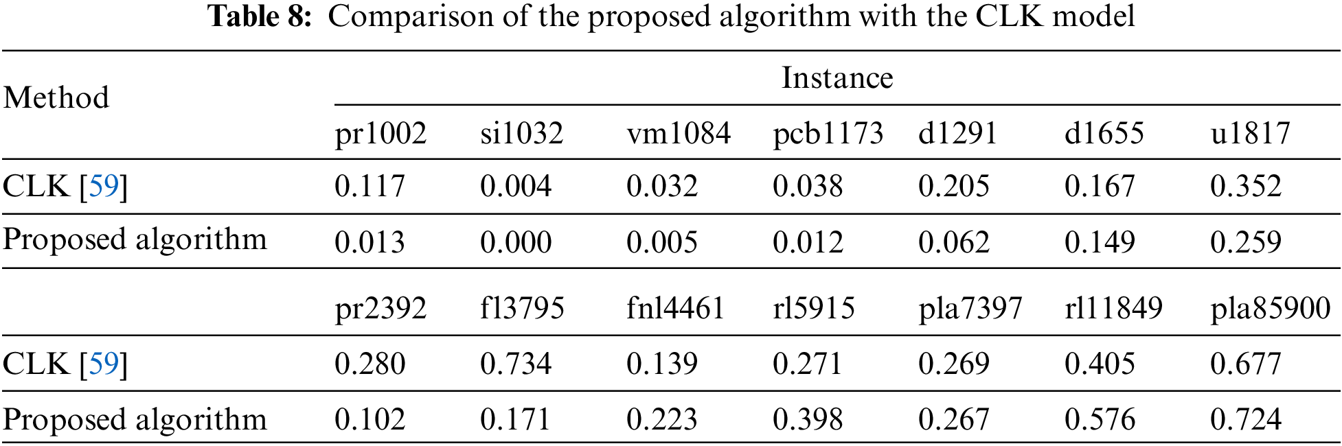
Table 8 compares the proposed algorithm with CLK. Both models use an LK local search strategy. By examining this comparison, it can be concluded that the proposed algorithm performs well in small-scale instances, while the CLK model performs better in large-scale cases. Wilcoxon signed-rank statistic test with a 95% confidence interval to evaluate the proposed algorithm’s performance compared to other algorithms.

The results of this test are shown in Table 9 based on the 95% confidence interval. These results show that the proposed algorithm performs well and significantly against the other 11 models: R+>R− and W≤WCri,N. Whereas we compared it with CLK, the result is as follows: W>WCri,N.

6  Conclusion and Future Works

This paper used the FFA algorithm to solve discrete problems such as the TSP problem. 10 LLHs were used to discretize this algorithm, which has generally led to the intelligent and automatic selection of LLHs using a hyper-heuristic mechanism based on MCF. Moreover, the following cases were performed: choosing the best solution in each sector and improving these solutions to focus more on the selected solutions. LK’s local search strategy improved the proposed algorithm’s performance. This paper presented and evaluated three models (MCF-FFA and (LLH4), MCF-FFA and Random-FFA). The MCF-FFA model showed better performance in most of the tested instances.

Due to the complex process of the proposed algorithm, it has been able to obtain quality solutions quickly. Achieving acceptable or quality results with simple procedures is no longer possible in the face of quality issues. We have tried to create a Multi-Start Local Search (MSLS) and Iterated Local Search (ILS) approach in the proposed algorithm. The proposed algorithm was tested with 71 cases with two criteria and compared with the 11 previously presented models, and the results indicated that the proposed algorithm is acceptable and appropriate. The proposed algorithm can be investigated and evaluated in the future to solve more advanced discrete problems such as travelling thief and vehicle routing problems (VRP). In addition, it is possible to design a version of the proposed algorithm to solve generic combinatorial optimization problems, which provides the ability to solve some well-known problems in the discrete problem space. Finally, the proposed algorithm can be generalized to solve discrete problems. To have the ability to solve multi-objective discrete problems and be evaluated.

Data Availability Statement (DAS): We use the available TSPLIB dataset for evaluation: http://comopt.ifi.uni-heidelberg.de/software/TSPLIB95/, 1991.

Funding Statement: The authors received no specific funding for this study.

Conflicts of Interest: The authors declare that they have no conflicts of interest to report regarding the present study.

References

1. Benyamin, A., Farhad, S. G., Saeid, B. (2021). Discrete farmland fertility optimization algorithm with metropolis acceptance criterion for traveling salesman problems. International Journal of Intelligent Systems, 36(3), 1270–1303. DOI 10.1002/int.22342. [Google Scholar] [CrossRef]
2. Gharehchopogh, F. S., Abdollahzadeh, B. (2022). An efficient Harris Hawk optimization algorithm for solving the travelling salesman problem. Cluster Computing, 25(3), 1981–2005. [Google Scholar]
3. Laporte, G., Nobert, Y. (1980). A cutting planes algorithm for the M-salesmen problem. Journal of the Operational Research Society, 31(11), 1017–1023. DOI 10.1057/jors.1980.188. [Google Scholar] [CrossRef]
4. Barnhart, C., Johnson, L. E., George, L. N., Martin, W. P. S., Pamela, H. V. (1998). Branch-and-price: Column generation for solving huge integer programs. Operations Research, 46(3), 316–329. DOI 10.1287/opre.46.3.316. [Google Scholar] [CrossRef]
5. Lawler, E. L., Wood, D. E. (1966). Branch-and-bound methods: A survey. Operations Research, 14(4), 699–719. DOI 10.1287/opre.14.4.699. [Google Scholar] [CrossRef]
6. Padberg, M., Rinaldi, G. (1987). Optimization of a 532-city symmetric traveling salesman problem by branch and cut. Operations Research Letters, 6(1), 1–7. DOI 10.1016/0167-6377(87)90002-2. [Google Scholar] [CrossRef]
7. Laporte, G. (1992). The traveling salesman problem: An overview of exact and approximate algorithms. European Journal of Operational Research, 59(2), 231–247. DOI 10.1016/0377-2217(92)90138-Y. [Google Scholar] [CrossRef]
8. Chakraborty, S., Saha, A. K., Chakraborty, R., Saha, M. (2021). An enhanced whale optimization algorithm for large scale optimization problems. Knowledge-Based Systems, 233, 107543. DOI 10.1016/j.knosys.2021.107543. [Google Scholar] [CrossRef]
9. Nama, S., Saha, A. K. (2019). A novel hybrid backtracking search optimization algorithm for continuous function optimization. Decision Science Letters, 8(2), 163–174. DOI 10.5267/j.dsl.2018.7.002. [Google Scholar] [CrossRef]
10. Zamani, H., Nadimi-Shahraki, M. H., Gandomi, A. H. (2021). QANA: Quantum-based avian navigation optimizer algorithm. Engineering Applications of Artificial Intelligence, 104, 104314. DOI 10.1016/j.engappai.2021.104314. [Google Scholar] [CrossRef]
11. Nadimi-Shahraki, M. H., Taghian, S., Mirjalili, S., Zamani, H., Bahreininejad, A. (2022). GGWO: Gaze cues learning-based grey wolf optimizer and its applications for solving engineering problems. Journal of Computational Science, 61, 101636. DOI 10.1016/j.jocs.2022.101636. [Google Scholar] [CrossRef]
12. Ezugwu, A. E. S., Adewumi, A. O., Fraoncu, M. E. (2017). Simulated annealing based symbiotic organisms search optimization algorithm for traveling salesman problem. Expert Systems with Applications, 77, 189–210. DOI 10.1016/j.eswa.2017.01.053. [Google Scholar] [CrossRef]
13. Saha, A. K. (2022). Multi-population-based adaptive sine cosine algorithm with modified mutualism strategy for global optimization. Knowledge-Based Systems, 109326. DOI 10.1016/j.knosys.2022.109326. [Google Scholar] [CrossRef]
14. Herrera, B. A. L. D. M., Coelho, L. D. S., Steiner, M. T. A. (2015). Quantum inspired particle swarm combined with Lin-Kernighan-Helsgaun method to the traveling salesman problem. Pesquisa Operacional, 35(3), 465–488. DOI 10.1590/0101-7438.2015.035.03.0465. [Google Scholar] [CrossRef]
15. Sahana, S. K. (2019). Hybrid optimizer for the travelling salesman problem. Evolutionary Intelligence, 12(2), 179–188. DOI 10.1007/s12065-019-00208-7. [Google Scholar] [CrossRef]
16. Marinakis, Y., Marinaki, M., Dounias, G. (2011). Honey bees mating optimization algorithm for the Euclidean traveling salesman problem. Information Sciences, 181(20), 4684–4698. DOI 10.1016/j.ins.2010.06.032. [Google Scholar] [CrossRef]
17. Gulcu, S., Mahi, M., Baykan, O. K., Kodaz, H. (2018). A parallel cooperative hybrid method based on ant colony optimization and 3-Opt algorithm for solving traveling salesman problem. Soft Computing, 22(5), 1669–1685. DOI 10.1007/s00500-016-2432-3. [Google Scholar] [CrossRef]
18. Burke, E. K., Gendreau, M., Hyde, M., Kendall, G., Ochoa, G. et al. (2013). Hyper-heuristics: A survey of the state of the art. Journal of the Operational Research Society, 64(12), 1695–1724. DOI 10.1057/jors.2013.71. [Google Scholar] [CrossRef]
19. Gharehchopogh, F. S. (2022). An improved tunicate swarm algorithm with best-random mutation strategy for global optimization problems. Journal of Bionic Engineering, 1–26. DOI 10.1007/s42235-022-00185-1. [Google Scholar] [CrossRef]
20. Gharehchopogh, F. S. (2022). Advances in tree seed algorithm: A comprehensive survey. Archives of Computational Methods in Engineering, 29, 3281–3330. DOI 10.1007/s11831-021-09698-0. [Google Scholar] [CrossRef]
21. Nadimi-Shahraki, M. H., Zamani, H. (2022). DMDE: Diversity-maintained multi-trial vector differential evolution algorithm for non-decomposition large-scale global optimization. Expert Systems with Applications, 198, 116895. DOI 10.1016/j.eswa.2022.116895. [Google Scholar] [CrossRef]
22. Zamani, H., Nadimi-Shahraki, M. H., Taghian, S., Dezfouli, M. B. (2020). Enhancement of bernstain-search differential evolution algorithm to solve constrained engineering problems. International Journal of Computer Science Engineering, 9, 386–396. [Google Scholar]
23. Zamani, H., Nadimi-Shahraki, M. H., Gandomi, A. H. (2019). CCSA: Conscious neighborhood-based crow search algorithm for solving global optimization problems. Applied Soft Computing, 85, 105583. DOI 10.1016/j.asoc.2019.105583. [Google Scholar] [CrossRef]
24. Nama, S., Sharma, S., Saha, A. K., Gandomi, A. H. (2022). A quantum mutation-based backtracking search algorithm. Artificial Intelligence Review, 55(4), 3019–3073. DOI 10.1007/s10462-021-10078-0. [Google Scholar] [CrossRef]
25. Chakraborty, S., Saha, A. K., Sharma, S., Chakraborty, R., Debnath, S. (2021). A hybrid whale optimization algorithm for global optimization. Journal of Ambient Intelligence and Humanized Computing. DOI 10.1007/s12652-021-03304-8. [Google Scholar] [CrossRef]
26. Nama, S., Saha, A. K. (2022). A bio-inspired multi-population-based adaptive backtracking search algorithm. Cognitive Computation, 14(2), 900–925. DOI 10.1007/s12559-021-09984-w. [Google Scholar] [CrossRef]
27. Nama, S., Saha, A. K., Sharma, S. (2022). A novel improved symbiotic organisms search algorithm. Computational Intelligence, 38(3), 947–977. DOI 10.1111/coin.12290. [Google Scholar] [CrossRef]
28. Azcan, E., Bilgin, B., Korkmaz, E. E. (2008). A comprehensive analysis of hyper-heuristics. Intelligent Data Analysis, 12(1), 3–23. DOI 10.3233/IDA-2008-12102. [Google Scholar] [CrossRef]
29. Lin, J., Wang, Z. J., Li, X. (2017). A backtracking search hyper-heuristic for the distributed assembly flow-shop scheduling problem. Swarm and Evolutionary Computation, 36, 124–135. DOI 10.1016/j.swevo.2017.04.007. [Google Scholar] [CrossRef]
30. Shayanfar, H., Gharehchopogh, F. S. (2018). Farmland fertility: A new metaheuristic algorithm for solving continuous optimization problems. Applied Soft Computing, 71, 728–746. DOI 10.1016/j.asoc.2018.07.033. [Google Scholar] [CrossRef]
31. Lin, S., Kernighan, B. W. (1973). An effective heuristic algorithm for the traveling-salesman problem. Operations Research, 21(2), 498–516. DOI 10.1287/opre.21.2.498. [Google Scholar] [CrossRef]
32. Reinelt, G. (1991). TSPLIB. http://www.iwr.uni-heidelberg.de/groups/comopt/software/TSPLIB95/. [Google Scholar]
33. Yong, W. (2015). Hybrid max–min ant system with four vertices and three lines inequality for traveling salesman problem. Soft Computing, 19(3), 585–596. DOI 10.1007/s00500-014-1279-8. [Google Scholar] [CrossRef]
34. Teng, L., Yin, S., Li, H. (2019). A new wolf colony search algorithm based on search strategy for solving travelling salesman problem. International Journal of Computational Science and Engineering, 18(1), 1–11. DOI 10.1504/IJCSE.2019.096970. [Google Scholar] [CrossRef]
35. Masutti, T. A., Decastro, L. N. (2009). A self-organizing neural network using ideas from the immune system to solve the traveling salesman problem. Information Sciences, 179(10), 1454–1468. DOI 10.1016/j.ins.2008.12.016. [Google Scholar] [CrossRef]
36. Luo, H., Xu, W., Tan, Y. (2018). A discrete fireworks algorithm for solving large-scale travel salesman problem. Proceedings of the 2018 IEEE Congress on Evolutionary Computation (CEC), pp. 1–7. Rio de Janeiro, Brazil, IEEE. [Google Scholar]
37. Cinar, A. C., Korkmaz, S., Kiran, M. S. (2019). A discrete tree-seed algorithm for solving symmetric traveling salesman problem. Engineering Science and Technology, An International Journal, 23(4), 879–890. DOI 10.1016/j.jestch.2019.11.005. [Google Scholar] [CrossRef]
38. Choong, S. S., Wong, L. P., Lim, C. P. (2019). An artificial bee colony algorithm with a modified choice function for the traveling salesman problem. Swarm and Evolutionary Computation, 44, 622–635. DOI 10.1016/j.swevo.2018.08.004. [Google Scholar] [CrossRef]
39. Ouaarab, A., Ahiod, B. D., Yang, X. S. (2015). Random-key cuckoo search for the travelling salesman problem. Soft Computing, 19(4), 1099–1106. DOI 10.1007/s00500-014-1322-9. [Google Scholar] [CrossRef]
40. Verma, O. P., Jain, R., Chhabra, V. (2014). Solution of travelling salesman problem using bacterial foraging optimisation algorithm. International Journal of Swarm Intelligence, 1(2), 179–192. DOI 10.1504/IJSI.2014.060243. [Google Scholar] [CrossRef]
41. Karaboga, D., Gorkemli, B. (2019). Solving traveling salesman problem by using combinatorial artificial Bee colony algorithms. International Journal on Artificial Intelligence Tools, 28(1), 1950004. DOI 10.1142/S0218213019500040. [Google Scholar] [CrossRef]
42. Zhong, Y., Lin, J., Wang, L., Zhang, H. (2018). Discrete comprehensive learning particle swarm optimization algorithm with metropolis acceptance criterion for traveling salesman problem. Swarm and Evolutionary Computation, 42, 77–88. DOI 10.1016/j.swevo.2018.02.017. [Google Scholar] [CrossRef]
43. Pook, M. F., Ramlan, E. I. (2019). The Anglerfish algorithm: A derivation of randomized incremental construction technique for solving the traveling salesman problem. Evolutionary Intelligence, 12(1), 11–20. DOI 10.1007/s12065-018-0169-x. [Google Scholar] [CrossRef]
44. Wang, Y., Wu, Y., Xu, N. (2019). Discrete symbiotic organism search with excellence coefficients and self-escape for traveling salesman problem. Computers & Industrial Engineering, 131, 269–281. DOI 10.1016/j.cie.2019.04.008. [Google Scholar] [CrossRef]
45. Ouaarab, A., Ahiod, B., Yang, X. S. (2014). Improved and discrete Cuckoo search for solving the travelling salesman problem. In: Cuckoo search and firefly algorithm, pp. 63–84. Springer, Cham. [Google Scholar]
46. Ezugwu, A. E. S., Adewumi, A. O. (2017). Discrete symbiotic organisms search algorithm for travelling salesman problem. Expert Systems with Applications, 87, 70–78. DOI 10.1016/j.eswa.2017.06.007. [Google Scholar] [CrossRef]
47. Yan, Y., Sohn, H. S., Reyes, G. (2017). A modified ant system to achieve better balance between intensification and diversification for the traveling salesman problem. Applied Soft Computing, 60, 256–267. DOI 10.1016/j.asoc.2017.06.049. [Google Scholar] [CrossRef]
48. Jiang, C., Wan, Z., Peng, Z. (2020). A new efficient hybrid algorithm for large scale multiple traveling salesman problems. Expert Systems with Applications, 139, 112867. DOI 10.1016/j.eswa.2019.112867. [Google Scholar] [CrossRef]
49. Chen, L., Sun, H. Y., Wang, S. (2012). A parallel ant colony algorithm on massively parallel processors and its convergence analysis for the travelling salesman problem. Information Sciences, 199, 31–42. DOI 10.1016/j.ins.2012.02.055. [Google Scholar] [CrossRef]
50. Ahmed, Z. H. (2014). Improved genetic algorithms for the travelling salesman problem. International Journal of Process Management and Benchmarking, 4(1), 109–124. DOI 10.1504/IJPMB.2014.059449. [Google Scholar] [CrossRef]
51. Lin, B. L., Sun, X., Salous, S. (2016). Solving travelling salesman problem with an improved hybrid genetic algorithm. Journal of Computer and Communications, 4(15), 98–106. DOI 10.4236/jcc.2016.415009. [Google Scholar] [CrossRef]
52. Wang, H., Zhang, N., Craoput, J. A. (2017). A massively parallel neural network approach to large-scale Euclidean traveling salesman problems. Neurocomputing, 240, 137–151. DOI 10.1016/j.neucom.2017.02.041. [Google Scholar] [CrossRef]
53. Zhong, Y., Lin, J., Wang, L., Zhang, H. (2017). Hybrid discrete artificial bee colony algorithm with threshold acceptance criterion for traveling salesman problem. Information Sciences, 421, 70–84. DOI 10.1016/j.ins.2017.08.067. [Google Scholar] [CrossRef]
54. Elkrari, M., Ahiod, B., Benani, E., Bouazza, Y. (2021). A pre-processing reduction method for the generalized travelling salesman problem. Operational Research, 21(4), 2543–2591. [Google Scholar]
55. Ayon; S. I., Akhand, M. A. H., Shahriyar, S. A., Siddique, N. (2019). Spider Monkey optimization to solve traveling salesman problem. 2019 International Conference on Electrical, Computer and Communication Engineering (ECCE), pp. 1–5. Cox’sBazar, Bangladesh, IEEE. [Google Scholar]
56. Cowling, P., Kendall, G., Soubeiga, E. (2000). A hyperheuristic approach to scheduling a sales summit. International Conference on the Practice and Theory of Automated Timetabling, pp. 176–190. Berlin, Heidelberg. [Google Scholar]
57. Cowling, P., Kendall, G., Soubeiga, E. (2001). A parameter-free hyperheuristic for scheduling a sales summit. Proceedings of the 4th Metaheuristic International Conference, pp. 127–131. Citeseer. [Google Scholar]
58. Marti, R. (2003). Multi-start methods. In: Handbook of metaheuristics, pp. 355–368. Boston, MA: Springer. [Google Scholar]
59. Applegate, D., Cook, W., Rohe, A. (2003). Chained Lin-kernighan for large traveling salesman problems. INFORMS Journal on Computing, 15(1), 82–92. DOI 10.1287/ijoc.15.1.82.15157. [Google Scholar] [CrossRef]
60. Martin, O., Otto, S. W., Felten, E. W. (1991). Large-step markov chains for the traveling salesman problem. Complex Systems, 5(3), 299–326. [Google Scholar]
61. Wilcoxon, F., Katti, S., Wilcox, R. A. (1970). Critical values and probability levels for the Wilcoxon rank sum test and the Wilcoxon signed rank test. Selected Tables in Mathematical Statistics, 1, 171–259. [Google Scholar]
62. Ismkhan, H. (2017). Effective heuristics for ant colony optimization to handle large-scale problems. Swarm and Evolutionary Computation, 32, 140–149. DOI 10.1016/j.swevo.2016.06.006. [Google Scholar] [CrossRef]
63. Tawhid, M. A., Savsani, P. (2019). Discrete sine-cosine algorithm (DSCA) with local search for solving traveling salesman problem. Arabian Journal for Science and Engineering, 44(4), 3669–3679. DOI 10.1007/s13369-018-3617-0. [Google Scholar] [CrossRef]
64. Zhong, Y., Wang, Y., Lin, M., Zhang, H. (2019). Discrete pigeon-inspired optimization algorithm with metropolis acceptance criterion for large-scale traveling salesman problem. Swarm and Evolutionary Computation, 48, 134–144. DOI 10.1016/j.swevo.2019.04.002. [Google Scholar] [CrossRef]
Cite This Article
Copyright © 2023 The Author(s). Published by Tech Science Press.
This work is licensed under a Creative Commons Attribution 4.0 International License , which permits unrestricted use, distribution, and reproduction in any medium, provided the original work is properly cited.
Downloads
Citation Tools