
 Submit a Paper
 Propose a Special lssue
 Open Access
ARTICLE

3D Vehicle Detection Algorithm Based on Multimodal Decision-Level Fusion
1 School of Mechanical Engineering, Anhui Polytechnic University, Wuhu, 241000, China
2 Department Polytechnic Institute of Zhejiang University, Hangzhou, 310000, China
* Corresponding Author: Peicheng Shi. Email:
Computer Modeling in Engineering & Sciences 2023, 135(3), 2007-2023. https://doi.org/10.32604/cmes.2023.022304
Received 03 March 2022; Accepted 01 August 2022; Issue published 23 November 2022
 View Full Text
 Download PDF
Abstract
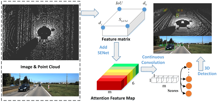
3D vehicle detection based on LiDAR-camera fusion is becoming an emerging research topic in autonomous driving. The algorithm based on the Camera-LiDAR object candidate fusion method (CLOCs) is currently considered to be a more effective decision-level fusion algorithm, but it does not fully utilize the extracted features of 3D and 2D. Therefore, we proposed a 3D vehicle detection algorithm based on multimodal decision-level fusion. First, project the anchor point of the 3D detection bounding box into the 2D image, calculate the distance between 2D and 3D anchor points, and use this distance as a new fusion feature to enhance the feature redundancy of the network. Subsequently, add an attention module: squeeze-and-excitation networks, weight each feature channel to enhance the important features of the network, and suppress useless features. The experimental results show that the mean average precision of the algorithm in the KITTI dataset is 82.96%, which outperforms previous state-of-the-art multimodal fusion-based methods, and the average accuracy in the Easy, Moderate and Hard evaluation indicators reaches 88.96%, 82.60%, and 77.31%, respectively, which are higher compared to the original CLOCs model by 1.02%, 2.29%, and 0.41%, respectively. Compared with the original CLOCs algorithm, our algorithm has higher accuracy and better performance in 3D vehicle detection.Graphic Abstract
Keywords
Nomenclature
| Camera external parameters | |
| Camera internal parameter |
With the development of autonomous driving in recent years, traditional 2D detection technology cannot support intelligent vehicle judgment of distance information, which affects the vehicle’s path planning and behavior decision-making. Therefore, 3D detection technology has attracted increasing attention from researchers. The 3D detection techniques include single-modality-based methods (camera and LiDAR) and multimodal fusion based methods. Camera images include rich color and texture information, but are sensitive to weather and lighting. LiDAR point clouds provide accurate depth and geometric structure information, which helps obtain the 3D pose of objects; however, point clouds are often sparse, and effectively extracting features becomes a challenge for LiDAR-based 3D detection. Hence, fusing the features of images and point clouds to achieve information redundancy and complementarity between modalities has become a current research focus.
According to the different locations where the fusion occurs, multimodal fusion methods can be divided into two classes according to [1]: feature fusion [2–4], and decision fusion [5–7], each of which has pros and cons. Feature fusion methods connect the information of different modes and perform joint reasoning, which allows cross-modal feature interactions. Prior MV3D [2] and AVOD [3] used region proposal networks (RPNs) to generate 3D regions of interest (ROI) by LiDAR specific views and image features and used them for class prediction and boundary box regression. However, LiDAR view selection is a core challenge in fusion. MVX-Net [8] projected point cloud voxel features into an image feature map and used RPNs to conduct 3D detection of the aggregated image and voxel features. This fusion method reduced the information loss caused by LiDAR view changes; however, the efficient alignment of point cloud features and images is challenging, and feature fusion often has a large computational complexity.
Decision-level fusion occurred in the final stage of the network and did not affect the individual predictions of each mode. Arnold et al. [9] evaluated three fusion methods and concluded that decision-level fusion has better performance than feature fusion methods. Cho et al. [5] introduced a new vision measurement model to obtain the target category and shape through vision, which improved the performance of data association and movement classification when the camera was fused with LiDAR. However, in complex scenarios, visual ranging shows large errors, resulting in decreased accuracy after fusion. Oh et al. [6] used convolutional neural networks (CNNs) to fuse the output results from LiDAR and image detectors, and finally output the category of each 2D detection result to achieve semantic consistency of visual category detection and LiDAR distance detection. This method provided a good idea for decision-level fusion, but did not verify the improvement of the algorithm for 3D detection performance. On this basis, the latest Camera-LiDAR object candidate fusion methods (CLOCs) [7] have been further explored by reducing the non-maximum suppression (NMS) [10] value of the two detectors, redundant candidate regions are obtained, and the 3D candidate regions are projected onto the RGB image. The fusion feature is established in the image, and then through a series of convolution operations, the score corresponding to each candidate area after the fusion is output, and the real vehicle target is finally detected based on the score. The core of CLOCs is to use 2D detection results to stimulate the detection potential of 3D detectors, which is efficient and flexible. However, CLOCs are based on data-driven fusion methods [11], and the challenge lies in the quantity and quality of input features. Specifically, the challenges of CLOCs are: (1) The features used to describe the relationship between 2D and 3D are single. (2) The importance of different features is ignored.
To address the challenges in CLOCs, we further improved CLOCs as shown in Fig. 1. For redundant LiDAR detection results, which include true positives with high confidence and false positives with low confidence, the key to CLOCs filtering false positives is to extract the intersection over union (IOU) of 2D and 3D detection boxes as fusion features. On this basis, we further explored the semantic consistency between 2D and 3D, enrich the number of fusion features by adding new

Figure 1: Further improvement of CLOCs
LiDAR point cloud-based methods dominate 3D object detection and are mainly divided into two categories: grid-based [12–14] and point-based methods [15–18]. These two methods are divided according to the different representations of the input data. Grid-based 3D detectors use a voxelized point cloud bird’s-eye view (BEV) perspective for detection, and in VoxelNet [12] and SECOND [13], they discretize the point cloud into a 3D grid, with each subspace called a voxel. Dense 3D points are represented using sparse voxels and applied to the network to learn features to detect. However, voxelization is expensive to process, and thus PointPillars [14] further reduce 3D voxels to 2D pillars for a BEV. The latest CenterPoint [19] uses this method as a backbone to extract features and uses a center point-based anchor-free detection head. For point-based methods, it mainly relies on PointNet++ [20] as the backbone to segment foreground points, and PointRCNN [15] and STD [16] perform two-stage detection boxes regression based on proposals generated by PointNet. Further, 3D SSD [17] proposes a point-based single-stage detector that handles upsampling layers and refinement modules. Point-based methods outperform grid-based methods in accuracy but require a higher computational load.
In recent years, multi-sensor fusion technology has shown great advantages. Based on the fusion stages that occur in the whole detection pipeline, they can be mainly divided into two categories: feature-level fusion [1–3] and decision-level fusion [5–7]. Feature-level fusion methods jointly perform joint inference on multi-sensor inputs. Early MV3D [2] and AVOD [3] fused point cloud features from different perspectives to generate two corresponding feature maps through feature extraction, and use RPN to generate the regional proposal. Wang et al. [1] added an attention module to the feature fusion. The network extracts multi-view features through three backbone networks, and then enters the attention mechanism module for fusion. It can be observed that adding an attention mechanism can effectively suppress noise interference. Feature-level fusion can fully perform feature interaction, but it is sensitive to the coordinate alignment accuracy between different modalities, and often cannot achieve modularity. Decision-level fusion, which is more flexible than feature fusion, utilizes image object detectors to generate 2D region proposals to compress ROI for 3D object detectors. The decision-level fusion method proposed by recent CLOCs [7] achieves state-of-the-art performance on the KITTI dataset [21], which exploits the spatial coherence of 2D and 3D, obtains fused features and uses continuous convolution to judge 3D detection results. However, CLOCs does not fully extract the relationship between point cloud and image, and do not further analyze the importance of point cloud and image features. On this basis, this study further enriches the fusion features of CLOCs and weights different feature channels.
To build a 3D vehicle detection network with good real-time performance and high accuracy, the backbone of the CLOCs [7] was selected and improved by adding feature dimensions and integrating attention modules. The improved network structure is shown in Fig. 2. First, the 2D image and 3D point cloud were input to each modal detector, and the fusion features were obtained according to the detection results. To enrich the fusion features of the network, based on the four-dimensional fusion features of the original CLOCs algorithm, in this study, we use the geometric consistency between different modalities to add a new one-dimensional distance feature. The feature is then convolved multiple times through our feature extraction networks and mapped to a higher-dimensional space. To improve the directivity of the feature, we use the channel attention module SENet [22] to assign weights to each feature channel, thereby enhancing important features in the network and suppressing useless features. Finally, the fused score map was outputted to judge the detection results. In this section, we describe our improvements in detail. Before that, we present and discuss the selection of 2D and 3D detectors.

Figure 2: Overall structure of improved CLOCs network
The selection of 2D and 3D detectors with excellent performance can provide high-quality input features for the network. In this study, we select YOLOv3 [23] as the 2D detector, and PointPillars [14] and PointRCNN [15] as 3D detectors based on weighing against the detection speed and mean average precision (mAP).
YOLOv3 is a detection network based on three prior bounding boxes, and its multi-scale prediction can provide more detailed features. YOLOv3 uses a 2D image as input, and outputs the bounding box, anchor point (center point) of the bounding box, and the confidence score of the detection target. As shown in Table 1, this evaluates YOLOv3 on the KITTI dataset [21]. The mAP can reach 89.54%, and the detection speed per frame is 0.07 s.
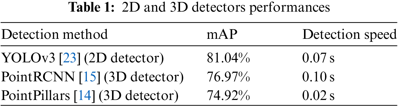
A 3D detector was used as the baseline for our network, combining the 2D detection results and generating the final 3D bounding box. To verify that our method is suitable for different 3D detectors, we select point-based PointRCNN and voxel-based PointPillars. PointRCNN uses PointNet++ [20] as the point cloud feature extractor, and proposes a bin-based 3D bounding box generation method that can provide accurate vehicle size and position information for our network. Different from PointRCNN, PointPillars implements 3D detection in a bird’s-eye-view. It extracts voxelized point cloud features and uses a feature pyramid network as a detection head for 3D detection box regression. Both 3D detectors take a 3D point cloud as input, and output the 3D bounding box, center point (anchor point) of the bounding box and confidence score of the detection object. As shown in Table 1, this study builds PointRCNN and PointPillars based on the OpenMMLab [24] platform to evaluate the KITTI dataset, their mAP can reach 76.97% and 74.92%, and the detection speed of each frame of the point cloud are 0.10 and 0.02 s, respectively.
3.2 Improved Fusion Features in CLOCs Algorithms
The main contributions of CLOCs include 1) proposing an effective decision-level fusion strategy, 2) obtaining redundant candidate regions by reducing the NMS threshold, and 3) constructing fusion features and learning the final prediction score. CLOCs will not affect the detection capacity of each modal at the decision-level, and simultaneously, they can fuse and correct the detection results; thus, the accuracy after fusion is superior compared to single-modal detection.
Following the CLOCs, we explored the impact of NMS on the 2D and 3D detection results. As shown in Fig. 2, 2D and 3D detectors are used to identify the point cloud and image in the same frame, and 3D and 2D bounding boxes are generated to determine the vehicle position and size. In CLOCs, it is believed that the detector suppresses true detection resulting in the later in NMS [10]; it is necessary to set a smaller NMS threshold to retain more candidate bounding boxes and reduce the missed detection of positive samples with low confidence. Hence, we further conducted a qualitative analysis. Fig. 3 shows the image and point cloud detection results for different NMS thresholds. As shown in Fig. 3a, YOLOv3 [23] is used for image detection. The upper side is the detection result when the NMS threshold is 0.5, and the lower side is the detection result when the NMS threshold is 0.25. It can be observed that when the NMS threshold is reduced, more bounding boxes with low confidence will be generated. Although the detection accuracy is reduced, redundancy of the candidate bounding boxes is achieved. In Fig. 3b, PointRCNN [15] is used for 3D detection; the left side shows the test result when NMS threshold is 0.7, and the right side shows the test result when NMS threshold is 0.2. It can be observed that after lowering the NMS threshold, there will be some positive test samples filtered out when the NMS threshold is 0.7, which can maximally increase the detection probability of potentially positive samples.

Figure 3: Change in NMS test results
After completing the 3D and 2D detections, the point cloud coordinates are onto the image according to the imaging principle of the camera. Assuming that the LiDAR coordinate system is the world coordinate system, according to Eq. (1), one point
where,
According to the output of the multimodal detector, the CLOCs proposed four fusion features. This study adds a one-dimensional distance feature on this basis. The specific acquisition steps of the fusion feature are as follows:
1) Fig. 4a shows a schematic of the projection of a 3D bounding box onto a 2D image, where the green bounding box is the 3D bounding box projection for point cloud detection and the red box is the 2D bounding box for image detection. The figure shows that when the 3D detection and 2D detection involve the same real sample, the box boundary overlaps and presents a large IoU. Therefore, the intersection ratio of the detection results of different modalities satisfies meets the requirements of the fusion feature, and a fusion feature can be formed.
2) Inspired by IoU features, in this study, we further explored the geometric relationship between 3D detection and 2D detection. The anchor point coordinates of the 3D detection bounding box are projected onto the image coordinate system using Eq. (1), as shown in Fig. 4b. Here, the green point represents the projection point of the anchor point of the 3D detection bounding box and the red point represents the anchor point of the 2D detection bounding box. It can be observed that the vehicle that is correctly detected by the 2D and 3D detectors simultaneously has a large IoU area and small anchor point spacing in the image. The IoU feature of the original CLOCs is the calculation of the intersection area of the 2D and 3D detection boxes (shaded area in Fig. 4c). Our

Figure 4: Obtaining fusion features
To verify the generalization of
3) To eliminate the interference of points located outside the camera’s field of view in network training, the normalized distance
4) The 2D and 3D detectors output the confidence score of each detection result based on the area of the target in the detection bounding box. The confidence score
By combining the above fusion features, we can build a sparse matrix, as shown in Eq. (3).

Figure 5: Anchor points spacing experiment
The dimension of the sparse matrix T is
3.3 SENet-Based Feature Extraction Networks
After completing the multimodal candidate feature collection, we construct a feature extraction network (FEN) to mine deeper semantics. Our FEN contains three layers of convolution and attention module SENet [22]. As shown in Fig. 2, the m non-empty element vectors are combined into a new feature matrix, and then three convolution operations are performed, all using
The high-dimensional features at this time have rich semantic information, but the features of these different modalities are messy, and thus we need to make the network adaptively learn more important features. Inspired by [1], adding an attention module can effectively estimate the importance of features and suppress noise features. Specifically, we consider the spatial attention module SAM [25], the channel attention module SENet [22], SPANet [26], and the combined attention module CBAM [27] in both ways. Through our experiments, SENet is finally selected as the attention module of our FEN. For a more detailed discussion, please refer to the experimental part of the next section.
The position of the SENet in the network is shown in Fig. 2. After the candidate feature matrix is convolved three times, the number of channels becomes 24, 48, and 96. The number of feature was the highest when the number of channels was 96. At this time, the addition of SENet results in maximum map region of the feature. After the weighted operation of SENet, features with different weights were outputted. The structure of the SENet module is shown in Fig. 6. The input feature layer size is

Figure 6: SENet structure diagram
Through the channel attention module SENet, each feature channel was weighted according to its role in the network. The feature vector was restored to the initial position of the sparse matrix according to the indicator. The score map containing each fusion target was mapped through max-pooling, and each vehicle fusion target corresponded to a probability of 0∼1 in the score map, which was used as the correct criterion for target detection.
4.1 Experimental Environment and Dataset
The operating system used in this experiment was Ubuntu 18.04, CPU was I7-10700, GeForce RTX 3060 graphics card was equipped, Python version 3.7.5, and the deep learning framework Pytorch 1.8.0.
The experiment adopted the KITTI dataset [21], which is a recognition algorithm evaluation dataset for an autonomous driving scenario. A total of 7,480 frames of images and point cloud data from different scenarios were selected as the dataset. During the training process, the dataset was divided into training set and validation set based on the ratio of 1:1. In the evaluation phase, the KITTI dataset was divided into three levels: easy, moderate, and hard, as evaluation metrics according to the degree of vehicle occlusion and truncation.
4.2 Optimizer, Loss Functions, and Metrics
In this study, a mini-batch was used on the optimizer to reduce the amount of calculation, the batch size was set to 1, the initial learning rate was 0.001, and Adam was used to optimizing the learning rate. After training 30 times, the learning rate was attenuated by 0.8 times. For instance, in Eq. (4), this study used the sigmoid focal loss function, which has superior performance in dealing with the problem of unbalanced simple samples and difficult samples, and has a good effect on the binary classification problems of vehicle detection [28].
where N represents the number of samples in the mini-batch,
To evaluate our method on the KITTI validation dataset, we used KITTI’s latest 3D object detection evaluation criteria with an average precision (AP) of 40-recall positions. For the average precision (AP) we follow the approach in [29] and define the AP as:
where
To verify the effectiveness of adding the


Figure 7: Loss curve comparison
To explore the influence of the number of convolution kernels and convolution layers on the network, we further adjusted different parameters to conduct orthogonal experiments. As shown in Table 3, we first used a smaller two-layer convolution and set the maximum number of channels to 36, as well as the mAP of the network to 81.11%. We then increased the number of convolutional layers and convolutional kernels to the parameters of the original CLOCs, at which time the mAP of the network increases by approximately two points. Increasing the number of convolution kernels, the mAP of the network changes less. However, note that when using three layers of convolution and a maximum of 96 convolution kernels, the network is effective for long distances (40∼50 m), and vehicle detection 3D AP is improved by 6.43% compared to the original CLOCs. Furthermore, when the number of convolutional layers is increased again, the mAP of the network and the 3D AP at different distance ranges no longer increase. This experiment guides the selection of our network parameters and verifies the effect of parameters on vehicle detection performance at different distances.

To quantitatively analyze the impact of different attention modules on our network, we compared SAM [25], CBAM [27], SENet [22] and SPANet [26] in terms of 3D AP and parameter size. As shown in Fig. 8, the spatial attention modules SAM and CBAM have a negative effect on the network, and the channel attention modules SENet and SPANet boost the benchmark 3D AP. SPANet outperforms SENet by 0.97% on 3D AP, but has three times as many parameters as SENet. Hence, after weighing the number of parameters and the improvement rate, we selected SENet as the attention module of our network.

Figure 8: Comparison of various attention modules
4.4 Algorithm Comparison Experiment
Currently, there are many types of 3D vehicle detection networks. To verify the effectiveness of the network in this study, a variety of popular 3D vehicle detection networks in the KITTI dataset list were selected for experimental comparison. In the single-modal detection, the SE-SSD [30], PointRCNN [15], SECOND [13] and PointPillars [14] networks were selected, whereas in the multimodal fusion network, PointPainting [31], 3D-CVF [32], AVOD [2] and CLOCs [7] networks were selected. For fuller quantitative analysis, we chose PointRCNN and PointPillars as 3D detector baselines to fuse with original CLOCs and our method. The evaluation results on the KITTI validation set are shown in Table 4. The bold numbers and blue numbers in Table 4 represent the first results and second results, respectively. Our method is slightly lower than the current state-of-the-art SE-SSD on vehicle detection on easy difficulty; however, it is worth noting that PointRCNN with our method outperforms SE-SSD on other metrics and achieves the best 82.95% 3D mAP and 90.42% BEV mAP. Whether it is PointRCNN or PointPillars baseline, our method yields a significant accuracy improvement, which proves the generalization of our method. In addition, we compare with the original CLOCs, for the PointPillars baseline, our method yields + 3.37% and + 3.07% gains on 3D mAP and BEV mAP (red numbers), respectively. In terms of running time, our method is efficient, the running time of the network mainly depends on the 3D detector with which it is fused, for PointRCNN and PointPillars, our method only slowed down by 12 and 17.9 ms, respectively.

Our method is also evaluated using the more challenging dataset: KITTI testing set; we submitted the test set prediction results to KITTI official for evaluation. In Table 5, it can be observed that our method mainly competes with AVOD-FPN [2] in a comprehensive performance. In the car class, our method is slightly lower than AVOD-FPN in car detection 3D AP on easy difficulty, where on moderate and hard difficulty, it outperforms other models.

4.5 Display of Detection Results
The detection results of this algorithm were tested visually. The image and point cloud data of the KITTI dataset were selected and detected using the network used in this study. The results are shown in Fig. 9. In the figure, the upper part is the point cloud detection result, and the red 3D bounding box is the real 3D bounding box. The green 3D bounding box is the detection of the 3D bounding box of this algorithm. For better visualization, the detected 3D bounding box is projected onto the 2D image below to generate a green 2D detection bounding box. Fig. 9a shows the 3D vehicle detection results for the unobstructed scenario. It can be observed that the network can correctly detect vehicles at different distances. Fig. 9b shows the detection results for the street scenario. It can be observed that the network can correctly detect vehicles with different degrees of occlusion and can detect positive samples without real labels. Fig. 9c shows the detection results for the road scenario. It can be observed that the network can correctly detect vehicles in different directions. However, for long-distance, heavily obscured incoming vehicles in the opposite direction, missed detections may occur. In summary, for vehicle targets in different scenarios, with different degrees of occlusion and distances, the network in this study can quickly and accurately complete the 3D detection of vehicles. Therefore, the improved CLOCs network proposed in this study is a multimodal fusion 3D vehicle detection network with good robustness and high accuracy.

Figure 9: Visualization of detection results
Because of the poor robustness and low accuracy of 3D vehicle detection in existing autonomous driving scenarios, a multimodal decision-level fusion method based on improved CLOCs was proposed.
(1) Project the 3D bounding box anchor points of the vehicle based on LiDAR detection into the 2D image and calculate the distance from the 2D bounding box anchor point of the vehicle detected by the camera; this distance is used as a new feature of the network to increase the input dimension of the network and enrich the integration characteristics of the network.
(2) Adding SENet-based feature extraction networks, adaptively adjusting the importance of each feature channel, assigning different weights to each feature channel, enhancing the important features of the network and suppressing useless special design can significantly improve the operating efficiency and learning capacity of the network.
(3) The experiments show that in 3D vehicle detection, the improved CLOCs algorithm can achieve average accuracies of 88.96%, 82.60%, and 77.31% in the three evaluation indicators of easy, moderate and hard, respectively, which are increased by 1.02%, 2.29% and 0.41%, respectively, compared with the original CLOCs algorithm.
(4) The algorithm proposed in this study uses only fixed 3D and 2D detectors for post-fusion. In future research, we will attempt to use different multimodal detectors to explore the impact of different detector performances on the algorithm and to optimize an optimal fusion strategy.
Funding Statement: This work was supported by the Financial Support of the Key Research and Development Projects of Anhui (202104a05020003), the Natural Science Foundation of Anhui Province (2208085MF173), and the Anhui Development and Reform Commission Supports R&D and Innovation Projects ([2020]479).
Conflicts of Interest: The authors declare that they have no conflicts of interest to report regarding the present study.
References
1. Wang, G., Tian, B., Zhang, Y., Chen, L., Cao, D. et al. (2020). Multi-view adaptive fusion network for 3D object detection. arXiv preprint arXiv:2011.00652. [Google Scholar]
2. Ku, J., Mozifian, M., Lee, J., Harakeh, A., Waslander, S. L. (2018). Joint 3D proposal generation and object detection from view aggregation. 2018 IEEE/RSJ International Conference on Intelligent Robots and Systems (IROS), pp. 1–8. Spain. [Google Scholar]
3. Chen, X., Ma, H., Wan, J., Li, B., Xia, T. (2017). Multi-view 3D object detection network for autonomous driving. Proceedings of the IEEE Conference on Computer Vision and Pattern Recognition, pp. 1907–1915. USA. [Google Scholar]
4. Liang, M., Yang, B., Chen, Y., Hu, R., Urtasun, R. (2019). Multi-task multi-sensor fusion for 3D object detection. Proceedings of the IEEE/CVF Conference on Computer Vision and Pattern Recognition, pp. 7345–7353. USA. [Google Scholar]
5. Cho, H., Seo, Y. W., Kumar, B. V., Rajkumar, R. R. (2014). A multi-sensor fusion system for moving object detection and tracking in urban driving environments. 2014 IEEE International Conference on Robotics and Automation (ICRA), pp. 1836–1843. Hong Kong, China. [Google Scholar]
6. Oh, S. I., Kang, H. B. (2017). Object detection and classification by decision-level fusion for intelligent vehicle systems. Sensors, 17(1), 207. DOI 10.3390/s17010207. [Google Scholar] [CrossRef]
7. Pang, S., Morris, D., Radha, H. (2020). CLOCs: Camera-LiDAR object candidates fusion for 3D object detection. 2020 IEEE/RSJ International Conference on Intelligent Robots and Systems (IROS), pp. 10386–10393. USA. [Google Scholar]
8. Sindagi, V. A., Zhou, Y., Tuzel, O. (2019). MVX-Net: Multimodal voxelnet for 3D object detection. 2019 International Conference on Robotics and Automation (ICRA), pp. 7276–7282. Canada. [Google Scholar]
9. Arnold, E., Al-Jarrah, O. Y., Dianati, M., Fallah, S., Oxtoby, D. et al. (2019). A survey on 3D object detection methods for autonomous driving applications. IEEE Transactions on Intelligent Transportation Systems, 20(10), 3782–3795. DOI 10.1109/TITS.6979. [Google Scholar] [CrossRef]
10. Neubeck, A., van Gool, L. (2006). Efficient non-maximum suppression. 18th International Conference on Pattern Recognition (ICPR), pp. 850–855. Hong Kong, China. [Google Scholar]
11. Chen, Q., Xie, Y., Ao, Y., Li, T., Chen, G. et al. (2021). A deep neural network inverse solution to recover pre-crash impact data of car collisions. Transportation Research Part C: Emerging Technologies, 126, 103009. DOI 10.1016/j.trc.2021.103009. [Google Scholar] [CrossRef]
12. Zhou, Y., Tuzel, O. (2018). VoxelNet: End-to-end learning for point cloud based 3D object detection. Proceedings of the IEEE Conference on Computer Vision and Pattern Recognition, pp. 4490–4499. USA. [Google Scholar]
13. Yan, Y., Mao, Y., Li, B. (2018). Second: Sparsely embedded convolutional detection. Sensors, 18(10), 3337. DOI 10.3390/s18103337. [Google Scholar] [CrossRef]
14. Lang, A. H., Vora, S., Caesar, H., Zhou, L., Yang, J. et al. (2019). PointPillars: Fast encoders for object detection from point clouds. Proceedings of the IEEE/CVF Conference on Computer Vision and Pattern Recognition, pp. 12697–12705. USA. [Google Scholar]
15. Shi, S., Wang, X., Li, H. (2019). PointRCNN: 3D object proposal generation and detection from point cloud. Proceedings of the IEEE/CVF Conference on Computer Vision and Pattern Recognition, pp. 770–779. USA. [Google Scholar]
16. Yang, Z., Sun, Y., Liu, S., Shen, X., Jia, J. (2019). STD: Sparse-to-dense 3D object detector for point cloud. Proceedings of the IEEE/CVF International Conference on Computer Vision, pp. 1951–1960. Korea. [Google Scholar]
17. Luo, Q., Ma, H., Tang, L., Wang, Y., Xiong, R. (2020). 3D-SSD: Learning hierarchical features from RGB-d images for amodal 3D object detection. Neurocomputing, 378, 364–374. DOI 10.1016/j.neucom.2019.10.025. [Google Scholar] [CrossRef]
18. Chen, P., Zhang, W., Xiao, Z., Tian, Y. (2022). Traffic accident detection based on deformable frustum proposal and adaptive space segmentation. Computer Modeling in Engineering & Sciences, 130(1), 97–109. DOI 10.32604/cmes.2022.016632. [Google Scholar] [CrossRef]
19. Yin, T., Zhou, X., Krahenbuhl, P. (2021). Center-based 3D object detection and tracking. Proceedings of the IEEE/CVF Conference on Computer Vision and Pattern Recognition, pp. 11784–11793. USA. [Google Scholar]
20. Qi, C. R., Yi, L., Su, H., Guibas, L. J. (2017). PointNet++: Deep hierarchical feature learning on point sets in a metric space. arXiv preprint arXiv:1706.02413, 2017. [Google Scholar]
21. Geiger, A., Lenz, P., Urtasun, R. (2012). Are we ready for autonomous driving? The KITTI vision benchmark suite. 2012 IEEE Conference on Computer Vision and Pattern Recognition, pp. 3354–3361. USA. [Google Scholar]
22. Hu, J., Shen, L., Sun, G. (2018). Squeeze-and-excitation networks. Proceedings of the IEEE Conference on Computer Vision and Pattern Recognition, pp. 7132–7141. USA. [Google Scholar]
23. Redmon, J., Farhadi, A. (2018). YOLOv3: An incremental improvement. arXiv preprint arXiv:1804.02767. [Google Scholar]
24. Chen, K., Wang, J., Pang, J., Cao, Y., Xiong, Y. et al. (2019). MMDetection: Open mmlab detection toolbox and benchmark. arXiv preprint arXiv:1906.07155. [Google Scholar]
25. Zhu, X., Cheng, D., Zhang, Z., Lin, S., Dai, J. (2019). An empirical study of spatial attention mechanisms in deep networks. Proceedings of the IEEE/CVF International Conference on Computer Vision, pp. 6688–6697. USA. [Google Scholar]
26. Guo, J., Ma, X., Sansom, A., McGuire, M., Kalaani, A. et al. (2020). Spanet: Spatial pyramid attention network for enhanced image recognition. 2020 IEEE International Conference on Multimedia and Expo (ICME), pp. 1–6. USA. [Google Scholar]
27. Woo, S., Park, J., Lee, J. Y., Kweon, I. S. (2018). Cbam: Convolutional block attention module. Proceedings of the European Conference on Computer Vision (ECCV), pp. 3–19. Germany. [Google Scholar]
28. Lin, T. Y., Goyal, P., Girshick, R., He, K., Dollár, P. (2017). Focal loss for dense object detection. Proceedings of the IEEE International Conference on Computer Vision, pp. 2980–2988. USA. [Google Scholar]
29. Simonelli, A., Bulo, S. R., Porzi, L., López-Antequera, M., Kontschieder, P. (2019). Disentangling monocular 3D object detection. Proceedings of the IEEE/CVF International Conference on Computer Vision, pp. 1991–1999. USA. [Google Scholar]
30. Zheng, W., Tang, W., Jiang, L., Fu, C. W. (2021). SE-SSD: Self-ensembling single-stage object detector from point cloud. Proceedings of the IEEE/CVF Conference on Computer Vision and Pattern Recognition, pp. 14494–14503. USA. [Google Scholar]
31. Vora, S., Lang, A. H., Helou, B., Beijbom, O. (2020). Pointpainting: Sequential fusion for 3D object detection. Proceedings of the IEEE/CVF Conference on Computer Vision and Pattern Recognition, pp. 4604–4612. USA. [Google Scholar]
32. Yoo, J. H., Kim, Y., Kim, J., Choi, J. W. (2020). 3D-CVF: Generating joint camera and lidar features using cross-view spatial feature fusion for 3D object detection. European Conference on Computer Vision, pp. 720–736. Glasgow. [Google Scholar]
33. Deng, J., Czarnecki, K. (2019). MLOD: A multi-view 3D object detection based on robust feature fusion method. 2019 IEEE Intelligent Transportation Systems Conference (ITSC), pp. 279–284. New Zealand. [Google Scholar]
34. Qi, C. R., Liu, W., Wu, C., Su, H., Guibas, L. J. (2018). Frustum pointnets for 3D object detection from RGB-D data. Proceedings of the IEEE Conference on Computer Vision and Pattern Recognition, pp. 918–927. USA. [Google Scholar]
Cite This Article
 Copyright © 2023 The Author(s). Published by Tech Science Press.
This work is licensed under a Creative Commons Attribution 4.0 International License , which permits unrestricted use, distribution, and reproduction in any medium, provided the original work is properly cited.
 Downloads
 Citation Tools