1 Introduction
The idea of metric dimension (MD) was firstly introduced by Melter et al. [1]. It has various applications in different areas such as the navigation system, image processing and drug discoveries. A network consists of nodes that are represented by vertices and connections between different vertices are denoted by edges. With the help of edges, an agent can change its position from one vertex to another. Some vertices are referred to as landmarks from which an agent can easily find its location in the network. The set with the minimum number of landmarks is known as the metric basis, and the cardinality of the aforesaid set is known as MD [2,3].
Moreover, the concept of MD in integer programming problem (IPP) was studied by Chartrand et al. [4]. Later on, Oellermann et al. [5,6] produced more refined results of (IPP) through MD. Fehr et al. [7] also derived various results for different graphs which are used to solve relaxation problems by using MD. For more results on MD, see [8,9].
The idea of fractional metric dimension (FMD) for different networks flourished through the work of Arumugam et al. [10]. Moreover, different networks are studied with the help of FMD such as hierarchical, Cartesian, corona, comb and lexicographic products [11–14]. Yi [15] and Liu et al. [16] calculated FMD for permutation and generalized Jahangir networks. Moreover, the sharps bounds of FMD for all the connected networks are studied in [17]. The idea of local fractional metric dimension (LFMD) came through the work of Aisyah et al. in which they computed the LFMD for the corona product of networks [18]. Later on, Liu et al. [19] discussed the LFMD for a particular class of planar networks called by circular ladders and rotationally symmetric networks. Recently, Javaid et al. calculated the bounds of LFMD of connected and prism related networks in [20,21].
In this paper, we find local resolving neighborhood sets (LRNs) of generalized Petersen network GP(n,3) for n≥5. After that, we calculated the sharp bounds of the local fractional metric dimension with the help of LRNs. The organization of paper is: Section 1 describes the introduction, Section 2 presents the preliminaries, Section 3 includes the local fractional metric dimensions of the Generalized Petersen network and Section 4 presents the discussion and conclusion.
2 Preliminaries
Mathematically, a network N consists of vertices set V(N)andedgessetE(N) with property E(N)⊆V(N)×V(N). In the present study, only the simple networks without any loop or parallel edges are considered. The distance between two vertices is considered as the length (number of edges) of the shortest path existing between them. For more basic notions, we refer to [22,23].
For any connected graph, y∈V(N) can resolve pair {v,w}∈V(N, if d(y,v)≠d(y,w). Let T be a set which is subset of V(N) known as resolving set of N if all pair of vertices in N are resolved by some vertices of T. The cardinality of resolving set is denoted by |T|. The set having minimum cardinality among all the resolving sets of N is called as metric dimension (MD).
For vw∈E(N), the local resolving neighborhood (LRN) set LR(vw) of vw is defined as LR(vw)={x∈V(N):d(x,v)≠d(x,w)}. A local resolving function (LRF) is a real valued function ϕ:V(N)→[0,1] such that ϕ(LR(vw))≥1 for each LR(vw) of N, where ϕ(LR(vw))=∑z∈LR(vw)ϕ(z). An LRF g is called minimal if there exists an other function ϕ:V(N)→[0,1] such that ϕ≤g and ϕ(u)≠g(u) for at least one u∈V, that is not a LRF of N. If |g|=∑y∈V(N)ϕ(x), then LFMD of N is defined as
dimlf(N)=min{|g|:g is a minimal LRF of N}. For more detail, see [1,10,19].
For n≥7, let GP(n,3) be a generalized Petersen network with vertex set V(GP(n,3))={xi,yj:1≤i,j≤n} and edge set E(GP(n,3))={xixi+1:1≤i≤n−1}∪{xiyi:1≤i≤n}∪{xnx1}∪{yiyi+3:1≤i≤n−3}∪{yn−2y1,yn−1y2,yny3}, where |V(GP(n,3))|=2n, |E(GP(n,3))|=3n (see Fig. 1).

Figure 1: Petersen graphs (a) GP(6, 3) and (b) GP(9, 3)
Now we present the following important result which will be frequently used in the main results.
Theorem 1: (see [15]) Let N(VN,E(N)) be a connected network and LR(c) be a local resolving neighborhood for some c∈E(N). If |LR(c)∩Y|≥α for all c∈E(N), then, dimlf(N)≤|Y|α, where, α=min{|LR(c)|:c∈E(N)}, Y=∪{LR(c):|LR(c)|=α}.
Theorem 2: (see [15]) For a connected network N, dimlf(N)=1 if N is bipartite.
Theorem 3: (see [20]) Let N(VN,E(N)) be a connected network and LR(c) be a local resolving neighborhood set. Then, |V(N|γ≤dimlf(N), where, γ=max{|LR(c)|:c∈E(N)} and 2≤γ≤|V(N)|.
3 Local Fractional Metric Dimension Generalized Petersen Network
This section deals with the main findings of the present studies.
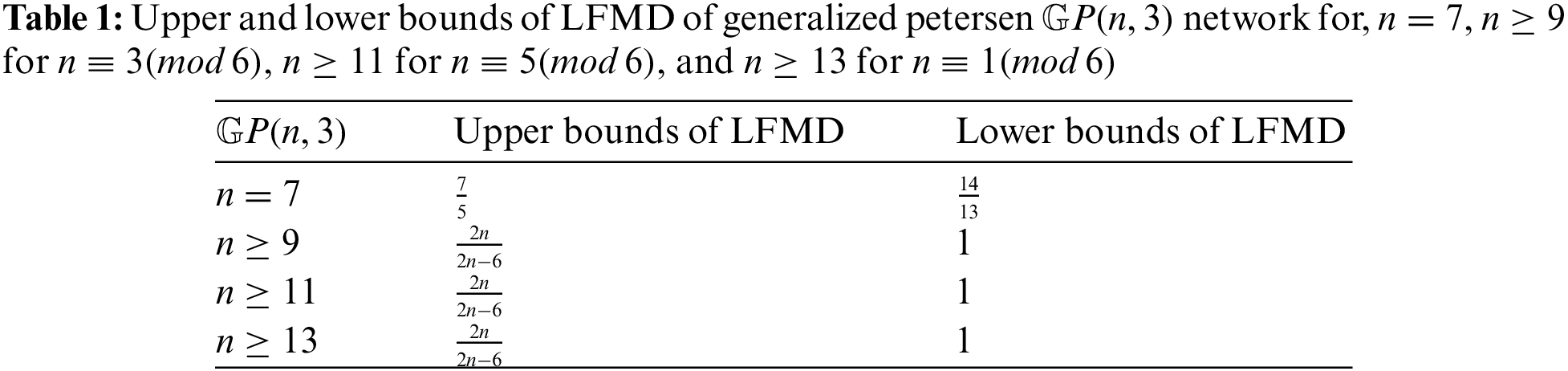
Theorem 4. The LFMD of generalized Petersen network GP(n,3) for n=7 is 1413≤dimlf(GP(7,3))≤75.
Proof: The LRNs of GP(n,3) for n=7 are given by:
LR1=LR(x1x2)=V(GP(7,3))−{x5,y5},LR2=LR(x2x3)=V(GP(7,3))−{x6,y6},
LR3=LR(x3x4)=V(GP(7,3))−{x7,y7},LR4=LR(x4x5)=V(GP(7,3))−{x1,y1},
LR5=LR(x5x6)=V(GP(7,3))−{x2,y2},LR6=LR(x6x7)=V(GP(7,3))−{x3,y3},
LR7=LR(x7x1)=V(GP(7,3))−{x4,y4},LR8=LR(y1y4)=V(GP(7,3))−{y6},
LR9=LR(y2y5)=V(GP(7,3))−{y7},LR10=LR(y3y6)=V(GP(7,3))−{y1},
LR11=LR(y4y7)=V(GP(7,3))−{y2},LR12=LR(y5y1)=V(GP(7,3))−{y3},
LR13=LR(y6y2)=V(GP(7,3))−{y4},LR14=LR(y7y3)=V(GP(7,3))−{y5},
LR(x1y1)=V(GP(7,3))−{y2,y3,y6,y7}=LR(e1),
LR(x2y2)=V(GP(7,3))−{y3,y4,y7,y1}=LR(e2),
LR(x3y3)=V(GP(7,3))−{y4,y5,y1,y2}=LR(e3),
LR(x4y4)=V(GP(7,3))−{y5,y6,y2,y3}=LR(e4),
LR(x5y5)=V(GP(7,3))−{y6,y7,y3,y4}=LR(e5),
LR(x6y6)=V(GP(7,3))−{y7,y1,y4,y5}=LR(e6),
LR(x7y7)=V(GP(7,3))−{y1,y2,y5,y6}=LR(e7).
For 1≤m≤14 and 1≤j≤7 LRN are |LR(ej)|=10<|LRm|. Furthermore, ∪j=17LR(ej)=V(GP(7,3)), |∪j=17LR(ej)|=14 and |LRm∩∪j=17LR(ej)|≥|LR(ej)|=10. Moreover, 1≤j≤7, LR(ej) are pairwise nonempty. There exist a minimal LRF ψ:V(GP(7,3))→[0,1] is defined as ψ(y)=110 for each y∈∪j=17LR(ej) and ψ(y)=0 for the vertices of GP(7,3) which are not in ∪j=17LR(ej). Therefore, by theorem 1, dimlf(GP(7,3))≤∑j=114110=1410. Since |V(GP(7,3))|=γ=13, then by Theorem 3 we have 1413≤dimlf(GP(7,3)) (as GP(7,3) is not bipartite network). Therefore, 1413≤dimlf(GP(n,3))≤75.
Lemma 1: Let GP(n,3) be Generalized Petersen network for, n≡3(mod6) and n≥9. Then, for 1≤i≤n−3, 1≤j≤n|LR(ej)|=|LR(ej=yiyi+3)|=2n−6=|LR(yn−2y1)|=|LR(yn−1y2)|=|LR(yny3)|. Moreover, ∪j=1nLR(ej)={xp:1≤p≤n}∪{yq:1≤q≤n} and |∪j=1nLR(ej)|=α=2n.
Proof: For, n≥9 and n≡3(mod6) the local resolving neighborhood of generalized Petersen network GP(n,3), for 1≤i≤n−3, 1≤j≤n, p,q≠n+32,n+52,n+72
LR(yiyi+3)={xp:1≤p≤nyq:1≤q≤n
with |LR(ej)|=2n−6 and ∪j=1nLR(ej)={xp:1≤p≤n}∪{yq:1≤q≤n} and we have |∪j=1nLR(ej)|=2n.
Lemma 2: Let GP(n,3) be generalized Petersen network with n≡3(mod6) and n≥9, then, for 1≤i≤n, 1≤j≤n. (a) |LR(ej)|<|LR(xixi+1)| and |LR(xixi+1)∩(∪j=1nLR(ej)|≥|LR(ej)|,
(b) |LR(ej)|<|LR(xiyi)| and |LR(xiyi)∩(∪j=1nLR(ej)|≥|LR(ej)|,
Proof: (a) The local resolving neighborhood for 1≤i≤n, 1≤j≤n, p,q≠n+32
LR(xixi+1)={xp:1≤p≤nyq:1≤q≤n
with |LR(xixi+1)|=2n−2>2n−6=|LR(ej)|, Therefore, |LR(xixi+1)∩(∪j=1nLRej)|=2n−2>|LR(ej)|.
(b) The local resolving neighborhood for 1≤i≤n, 1≤j≤n,
LR(xiyi)={xp:1≤p≤nyq:1≤q≤n
with |LR(xiyi)|=2n>2n−6=|LR(ej)|, Therefore, |LR(xiyi)∩(∪j=1nLRej)|=2n>|LR(ej)|.
Theorem 5: Let GP(n,3) with n≡3(mod6) be a generalized Petersen network, where |V(GP(n,3))|=2n and n≥9. Then, 1≤dimlf(GP(n,3))≤2n2n−6.
Proof:
Case 1: The LRNs of GP(n,3) for n=9 are given by:
LR1=LR(x1x2)=V(GP(9,3))−{x6,y6},LR2=LR(x2x3)=V(GP(9,3))−{x7,y7},
LR3=LR(x3x4)=V(GP(9,3))−{x8,y8},LR4=LR(x4x5)=V(GP(9,3))−{x9,y9},
LR5=LR(x5x6)=V(GP(9,3))−{x1,y1},LR6=LR(x6x7)=V(GP(9,3))−{x2,y2},
LR7=LR(x7x8)=V(GP(9,3))−{x3,y3},LR8=LR(x8x9)=V(GP(9,3))−{x4,y4},
LR9=LR(x9x1)=V(GP(9,3))−{x5,y5},LR10=LR(x1y1)=V(GP(9,3)),
LR11=LR(x2y2)=V(GP(9,3)),LR12=LR(x3y3)=V(GP(9,3)),
LR13=LR(x4y4)=V(GP(9,3)),LR14=LR(x5y5)=V(GP(9,3)),
LR15=LR(x6y6)=V(GP(9,3)),LR16=LR(x7y7)=V(GP(9,3)),
LR17=LR(x8y8)=V(GP(9,3)),LR18=LR(x9y9)=V(GP(9,3)),
LR(y1y4)=V(GP(9,3))−{x6,x7,x8,y6,y7,y8}=LR(e1),
LR(y2y5)=V(GP(9,3))−{x7,x8,x9,y7,y8,y9}=LR(e2),
LR(y3y6)=V(GP(9,3))−{x8,x9,x1,y8,y9,y1}=LR(e3),
LR(y4y7)=V(GP(9,3))−{x9,x1,x2,y9,y1,y2}=LR(e4),
LR(y5y8)=V(GP(9,3))−{x1,x2,x3,y1,y2,y3}=LR(e5),
LR(y6y9)=V(GP(9,3))−{x2,x3,x4,y2,y3,y4}=LR(e6),
LR(y7y1)=V(GP(9,3))−{x3,x4,x5,y3,y4,y5}=LR(e7),
LR(y8y2)=V(GP(9,3))−{x4,x5,x6,y4,y5,y6}=LR(e8),
LR(y9y3)=V(GP(9,3))−{x5,x6,x7,y5,y6,y7}=LR(e9).
For 1≤m≤18 and 1≤j≤9 LRN are |LR(ej)|=12<|LRm|. Furthermore, ∪j=19LR(ej)=V(GP(9,3)), |∪j=19LR(ej)|=18 and |LRm∩∪j=19LR(ej)|≥|LR(ej)|=12. Moreover, 1≤j≤9, LR(ej) are pairwise nonempty. There exist a minimal LRF ψ:V(GP(9,3))→[0,1] is defined as ψ(y)=112 for each y∈∪j=19LR(ej) and ψ(y)=0 for the vertices of GP(9,3) which are not in ∪j=19LR(ej). Therefore, by Theorem 1, dimlf(GP(9,3))≤∑j=1181812=32. Since |V(GP(9,3))|=γ=18, then by Theorem 3 1818≤dimlf(GP(9,3)) implies 1≤dimlf(GP(9,3)) (as GP(9,3) is not bipartite network). Therefore, 1≤dimlf(GP(9,3))≤32.
Case 2: The LRNs of GP(n,3) for n=15 are given by:
LR1=LR(x1x2)=V(GP(15,3))−{x9,y9},LR2=LR(x2x3)=V(GP(15,3))−{x10,y10},
LR3=LR(x3x4)=V(GP(15,3))−{x11,y11},LR4=LR(x4x5)=V(GP(15,3))−{x12,y12},
LR5=LR(x5x6)=V(GP(15,3))−{x13,y13},LR6=LR(x6x7)=V(GP(15,3))−{x14,y14},
LR7=LR(x7x8)=V(GP(15,3))−{x15,y15},LR8=LR(x8x9)=V(GP(15,3))−{x1,y1},
LR9=LR(x9x10)=V(GP(15,3))−{x2,y2},LR10=LR(x10x11)=V(GP(15,3))−{x3,y3},
LR11=LR(x11x12)=V(GP(15,3))−{x4,y4},LR12=LR(x12x13)=V(GP(15,3))−{x5,y5},
LR13=LR(x13x14)=V(GP(15,3))−{x6,y6},LR14=LR(x14x15)=V(GP(15,3))−{x7,y7},
LR15=LR(x15x1)=V(GP(15,3))−{x8,y8},LR16=LR(x1y1)=V(GP(15,3)),
LR17=LR(x2y2)=V(GP(15,3)),LR18=LR(x3y3)=V(GP(15,3)),
LR19=LR(x4y4)=V(GP(15,3)),LR20=LR(x5y5)=V(GP(15,3)),
LR21=LR(x6y6)=V(GP(15,3)),LR22=LR(x7y7)=V(GP(15,3)),
LR23=LR(x8y8)=V(GP(15,3)),LR24=LR(x9y9)=V(GP(15,3)),
LR25=LR(x10y10)=V(GP(15,3)),LR26=LR(x11y11)=V(GP(15,3)),
LR27=LR(x12y12)=V(GP(15,3)),LR28=LR(x13y13)=V(GP(15,3)),
LR29=LR(x14y14)=V(GP(15,3)),LR30=LR(x15y15)=V(GP(15,3)),
LR(y1y4)=V(GP(15,3))−{x9,x10,x11,y9,y10,y11}=LR(e1),
LR(y2y5)=V(GP(15,3))−{x10,x11,x12,y10,y11,y12}=LR(e2),
LR(y3y6)=V(GP(15,3))−{x11,x12,x13,y11,y12,y13}=LR(e3),
LR(y4y7)=V(GP(15,3))−{x12,x13,x14,y12,y13,y14}=LR(e4),
LR(y5y8)=V(GP(15,3))−{x13,x14,x15,y13,y14,y15}=LR(e5),
LR(y6y9)=V(GP(15,3))−{x14,x15,x1,y14,y15,y1}=LR(e6),
LR(y7y10)=V(GP(15,3))−{x15,x1,x2,y15,y1,y2}=LR(e7),
LR(y8y11)=V(GP(15,3))−{x1,x2,x3,y1,y2,y3}=LR(e8),
LR(y9y12)=V(GP(15,3))−{x2,x3,x4,y2,y3,y4}=LR(e9),
LR(y10y13)=V(GP(15,3))−{x3,x4,x5,y3,y4,y5}=LR(e10),
LR(y11y14)=V(GP(15,3))−{x4,x5,x6,y4,y5,y6}=LR(e11),
LR(y12y15)=V(GP(15,3))−{x5,x6,x7,y5,y6,y7}=LR(e12),
LR(y13y1)=V(GP(15,3))−{x6,x7,x8,y6,y7,y8}=LR(e13),
LR(y14y2)=V(GP(15,3))−{x7,x8,x9,y7,y8,y9}=LR(e14),
LR(y15y3)=V(GP(15,3))−{x8,x9,x10,y8,y9,y10}=LR(e15).
For 1≤m≤30 and 1≤j≤15 LRN are |LR(ej)|=24<|LRm|. Furthermore, ∪j=115LR(ej)=V(GP(15,3)), |∪j=115LR(ej)|=30 and |LRm∩∪j=115LR(ej)|≥|LR(ej)|=24. Moreover, 1≤j≤15, LR(ej) are pairwise nonempty. There exist a minimal LRF ψ:V(GP(15,3))→[0,1] is defined as ψ(y)=124 for each y∈∪j=115LR(ej) and ψ(y)=0 for the vertices of GP(15,3) which are not in ∪j=115LR(ej). Therefore, by Theorem 1, dimlf(GP(15,3))≤∑j=1303020=54. Since |V(GP(15,3))|=γ=30, then by Theorem 3 we have 3030≤dimlf(GP(15,3)) implies 1≤dimlf(GP(15,3)). As GP(15,3) is not bipartite network therefore, 1≤dimlf(GP(15,3))≤54.
Case 3: For 1≤i≤n, 1≤j≤n and n≥19, LR(ej)=LR(yiyi+3), LR(xixi+1), LR(xiyi). By Lemmas 1, 2, we have (i) |LR(xixi+1)|,LR(xiyi)≥|LR(ej)|=2n−6=α, (ii) |LR(xixi+1)∩∪j=1nLR(ej)|, |LR(xiyi)∩∪j=1nLR(ej)|≥|LR(ej)| and ∪j=1nLR(ej)=2n=β. The intersection of LRS having minimum cardinality is not empty. Therefore, there exist a mimimal local resolving ψ′:V(GP(n,3))→[0,1] such that |ψ′|<|ψ|, where the minimal LRF ψ:V(GP(n,3))→[0,1] is defined as ϕ(v)={1αforv∈∪j=1nLR(ej)}.
Therefore, by Theorem 1, dimlf(GP(n,3))≤∑t=1β1α=2n2n−6. Since |V(GP(n,3))|=γ=2n, then by Theorem 3 we have 2n2n≤dimlf(GP(n,3)) implies 1≤dimlf(GP(n,3)). As GP(n,3) is not bipartite network therefore, 1≤dimlf(GP(n,3))≤2n2n−6.
Lemma 3: Let GP(n,3) be Generalized Petersen network for, n≡3(mod6) and n≥11. Then, for 1≤i≤n−3, 1≤j≤n|LR(ej)|=|LR(ej=yiyi+3)|=2n−6=|LR(yn−2y1)|=|LR(yn−1y2)|=|LR(yny3)|. Moreover, ∪j=1nLR(ej)={xp:1≤p≤n}∪{yq:1≤q≤n} and |∪j=1nLR(ej)|=α=2n.
Proof: For, n≥11 and n≡3(mod6) the local resolving neighborhood of generalized Petersen network GP(n,3), for 1≤i≤n−3, 1≤j≤n, p≠n+12,n+52,n+92, q≠n−52,n+52,n+152,
LR(yiyi+3)={xp:1≤p≤nyq:1≤q≤n
with |LR(ej)|=2n−6 and ∪j=1nLR(ej)={xp:1≤p≤n}∪{yq:1≤q≤n} and we have |∪j=1nLR(ej)|=2n.
Lemma 4: Let GP(n,3) be generalized Petersen network with n≡3(mod6) and n≥11, then, for 1≤i≤n, 1≤j≤n.
(a) |LR(ej)|<|LR(xixi+1)| and |LR(xixi+1)∩(∪j=1nLR(ej)|≥|LR(ej)|,
(b) |LR(ej)|<|LR(xiyi)| and |LR(xiyi)∩(∪j=1nLR(ej)|≥|LR(ej)|,
Proof: (a) The local resolving neighborhood for 1≤i≤n, 1≤j≤n, p,q≠n+32
LR(xixi+1)={xp:1≤p≤nyq:1≤q≤n
with |LR(xixi+1)|=2n−2>2n−6=|LR(ej)|, Therefore, |LR(xixi+1)∩(∪j=1nLRej)|=2n−2>|LR(ej)|.
(b) The local resolving neighborhood for 1≤i≤n, 1≤j≤n,
LR(xiyi)={xp:1≤p≤nyq:1≤q≤n
with |LR(xiyi)|=2n>2n−6=|LR(ej)|, Therefore, |LR(xiyi)∩(∪j=1nLRej)|=2n>|LR(ej)|.
Theorem 6: Let GP(n,3)n≡5(mod6) be a generalized Petersen network, where |V(GP(n,2))|=2n and n≥11. Then, 1≤dimlf(GP(n,3))≤2n2n−6.
Proof:
The LRNs of GP(n,3) for n=11 are given by:
LR1=LR(x1x2)=V(GP(11,3))−{x7,y7},LR2=LR(x2x3)=V(GP(11,3))−{x8,y8},
LR3=LR(x3x4)=V(GP(11,3))−{x9,y9},LR4=LR(x4x5)=V(GP(11,3))−{x10,y10},
LR5=LR(x5x6)=V(GP(11,3))−{x11,y11},LR6=LR(x6x7)=V(GP(11,3))−{x1,y1},
LR7=LR(x7x8)=V(GP(11,3))−{x2,y2},LR8=LR(x8x9)=V(GP(11,3))−{x3,y3},
LR9=LR(x9x10)=V(GP(11,3))−{x4,y4},LR10=LR(x10x11)=V(GP(11,3))−{x5,y5},
LR11=LR(x11x1)=V(GP(11,3))−{x6,y6},LR12=LR(x1y1)=V(GP(11,3)),
LR13=LR(x2y2)=V(GP(11,3)),LR14=LR(x3y3)=V(GP(11,3)),
LR15=LR(x4y4)=V(GP(11,3)),LR16=LR(x5y5)=V(GP(11,3)),
LR17=LR(x6y6)=V(GP(11,3)),LR18=LR(x7y7)=V(GP(11,3)),
LR19=LR(x8y8)=V(GP(11,3)),LR20=LR(x9y9)=V(GP(11,3)),
LR21=LR(x10y10)=V(GP(11,3)),LR22=LR(x11y11)=V(GP(11,3)),
LR(y1y4)=V(GP(11,3))−{x6,x8,x10,y2,y3,y8}=LR(e1),
LR(y2y5)=V(GP(11,3))−{x7,x9,x11,y3,y4,y9}=LR(e2),
LR(y3y6)=V(GP(11,3))−{x8,x10,x1,y4,y5,y10}=LR(e3),
LR(y4y7)=V(GP(11,3))−{x9,x11,x2,y5,y6,y11}=LR(e4),
LR(y5y8)=V(GP(11,3))−{x10,x1,x3,y6,y7,y1}=LR(e5),
LR(y6y9)=V(GP(11,3))−{x11,x2,x4,y7,y8,y2}=LR(e6),
LR(y7y10)=V(GP(11,3))−{x1,x3,x5,y8,y9,y3}=LR(e7),
LR(y8y11)=V(GP(11,3))−{x2,x4,x6,y9,y10,y4}=LR(e8),
LR(y9y1)=V(GP(11,3))−{x3,x5,x7,y10,y11,y5}=LR(e9),
LR(y10y2)=V(GP(11,3))−{x4,x6,x8,y11,y1,y6}=LR(e10),
LR(y11y3)=V(GP(11,3))−{x5,x7,x9,y1,y2,y7}=LR(e11).
For 1≤m≤22 and 1≤j≤11 LRN are |LR(ej)|=16<|LRm|. Furthermore, ∪j=111LR(ej)=V(GP(11,2)), |∪j=111LR(ej)|=22 and |LRm∩∪j=111LR(ej)|≥|LR(ej)|=16. Moreover, 1≤j≤11, LR(ej) are pairwise nonempty. There exist a minimal LRF ψ:V(GP(14,2))→[0,1] is defined as ψ(y)=116 for each y∈∪j=111LR(ej) and ψ(y)=0 for the vertices of GP(11,3) which are not in ∪j=114LR(ej). Therefore, by Theorem 1, dimlf(GP(11,3))≤∑j=122116=118. Since |V(GP(11,3))|=γ=22, then by Theorem 3 we have 2222≤dimlf(GP(11,3)) implies 1≤dimlf(GP(11,3)). As GP(11,3) is not bipartite network therefore, 1≤dimlf(GP(11,3))≤118.
Case 2: The LRNs of GP(n,3) for n=17 are given by:
LR1=LR(x1x2)=V(GP(17,3))−{x10,y10},LR2=LR(x2x3)=V(GP(17,3))−{x11,y11},
LR3=LR(x3x4)=V(GP(17,3))−{x12,y12},LR4=LR(x4x5)=V(GP(17,3))−{x13,y13},
LR5=LR(x5x6)=V(GP(17,3))−{x14,y14},LR6=LR(x6x7)=V(GP(17,3))−{x15,y15},
LR7=LR(x7x8)=V(GP(17,3))−{x16,y16},LR8=LR(x8x9)=V(GP(17,3))−{x17,y17},
LR9=LR(x9x10)=V(GP(17,3))−{x1,y1},LR10=LR(x10x11)=V(GP(17,3))−{x2,y2},
LR11=LR(x11x12)=V(GP(17,3))−{x3,y3},LR12=LR(x12x13)=V(GP(17,3))−{x4,y4},
LR13=LR(x13x14)=V(GP(17,3))−{x5,y5},LR14=LR(x14x15)=V(GP(17,3))−{x6,y6},
LR15=LR(x15x16)=V(GP(17,3))−{x7,y7},LR16=LR(x16x17)=V(GP(17,3))−{x8,y8},
LR17=LR(x17x1)=V(GP(17,3))−{x9,y9},LR18=LR(x1y1)=V(GP(17,3)),
LR19=LR(x2y2)=V(GP(17,3)),LR20=LR(x3y3)=V(GP(17,3)),
LR21=LR(x4y4)=V(GP(17,3)),LR22=LR(x5y5)=V(GP(17,3)),
LR23=LR(x6y6)=V(GP(17,3)),LR24=LR(x7y7)=V(GP(17,3)),
LR25=LR(x8y8)=V(GP(17,3)),LR26=LR(x9y9)=V(GP(17,3)),
LR27=LR(x10y10)=V(GP(17,3)),LR28=LR(x11y11)=V(GP(17,3)),
LR29=LR(x12y12)=V(GP(17,3)),LR30=LR(x13y13)=V(GP(17,3)),
LR31=LR(x14y14)=V(GP(17,3)),LR32=LR(x15y15)=V(GP(17,3)),
LR33=LR(x16y16)=V(GP(17,3)),LR34=LR(x17y17)=V(GP(17,3)),
LR(y1y4)=V(GP(17,3))−{x9,x11,x13,y6,y11,y16}=LR(e1),
LR(y2y5)=V(GP(17,3))−{x10,x12,x14,y7,y12,y17}=LR(e2),
LR(y3y6)=V(GP(17,3))−{x11,x13,x15,y8,y13,y1}=LR(e3),
LR(y4y7)=V(GP(17,3))−{x12,x14,x16,y9,y14,y2}=LR(e4),
LR(y5y8)=V(GP(17,3))−{x13,x15,x17,y10,y15,y3}=LR(e5),
LR(y6y9)=V(GP(17,3))−{x14,x16,x1,y11,y16,y4}=LR(e6),
LR(y7y10)=V(GP(17,3))−{x15,x17,x2,y12,y17,y5}=LR(e7),
LR(y8y11)=V(GP(17,3))−{x16,x1,x3,y13,y1,y6}=LR(e8),
LR(y9y12)=V(GP(17,3))−{x17,x2,x4,y14,y2,y7}=LR(e9),
LR(y10y13)=V(GP(17,3))−{x1,x3,x5,y15,y3,y8}=LR(e10),
LR(y11y14)=V(GP(17,3))−{x2,x4,x6,y16,y4,y9}=LR(e11),
LR(y12y15)=V(GP(17,3))−{x3,x5,x7,y17,y5,y10}=LR(e12),
LR(y13y16)=V(GP(17,3))−{x4,x6,x8,y1,y6,y11}=LR(e13),
LR(y14y17)=V(GP(17,3))−{x5,x7,x9,y2,y7,y12}=LR(e14),
LR(y15y1)=V(GP(17,3))−{x6,x8,x10,y3,y8,y13}=LR(e15),
LR(y16y2)=V(GP(17,3))−{x7,x9,x11,y4,y9,y14}=LR(e16),
LR(y17y3)=V(GP(17,3))−{x8,x10,x12,y5,y10,y15}=LR(e17).
For 1≤m≤34 and 1≤j≤17 LRN are |LR(ej)|=28<|LRm|. Furthermore, ∪j=117LR(ej)=V(GP(17,3)), |∪j=117LR(ej)|=34 and |LRm∩∪j=117LR(ej)|≥|LR(ej)|=28. Moreover, 1≤j≤17, LR(ej) are pairwise nonempty. There exist a minimal LRF ψ:V(GP(17,3))→[0,1] is defined as ψ(y)=128 for each y∈∪j=117LR(ej) and ψ(y)=0 for the vertices of GP(17,3) which are not in ∪j=117LR(ej). Therefore, by Theorem 1, dimlf(GP(17,3))≤∑j=134124=1714.
dimlf(GP(17,3))≤1714.
Case 3: For 1≤i≤n, 1≤j≤n and n≥23, LR(ej)=LR(yiyi+3), LR(xixi+1), LR(xiyi). By Lemmas 3, 4, we have (i) |LR(xixi+1)|, LR(xiyi)≥|LR(ej)|=2n−6=α, (ii) |LR(xixi+1)∩∪j=1nLR(ej)|, |LR(xiyi)∩∪j=1nLR(ej)|≥|LR(ej)| and ∪j=1nLR(ej)=2n=β. The intersection of LRS having minimum cardinality is not empty. Therefore, there exist a mimimal local resolving ψ′:V(GP(n,3))→[0,1] such that |ψ′|<|ψ|, where the minimal LRF ψ:V(GP(n,3))→[0,1] is defined as ϕ(v)={1αforv∈∪j=1nLR(ej)}.
Therefore, by Theorem 1, dimlf(GP(n,3))≤∑t=1β1α=2n2n−6. Since |V(GP(n,3))|=γ=2n, then by Theorem 3 we have 2n2n≤dimlf(GP(n,3)) implies 1≤dimlf(GP(n,3)). As GP(n,3) is not bipartite network therefore, 1≤dimlf(GP(n,3))≤2n2n−6.
Lemma 5: Let GP(n,3) be Generalized Petersen network for, n≡1(mod6) and n≥13. Then, for 1≤i≤n−3, 1≤j≤n|LR(ej)|=|LR(ej=yiyi+3)|=2n−6=|LR(yn−2y1)|=|LR(yn−1y2)|=|LR(yny3)|. Moreover, ∪j=1nLR(ej)={xp:1≤p≤n}∪{yq:1≤q≤n} and |∪j=1nLR(ej)|=α=2n.
Proof: For, n≥13 and n≡3(mod6) the local resolving neighborhood of generalized Petersen network GP(n,3), for 1≤i≤n−3, 1≤j≤n, p≠n+32,n+52,n+72, q≠n−32,n+52,n+132,
LR(yiyi+3)={xp:1≤p≤nyq:1≤q≤n
with |LR(ej)|=2n−6 and ∪j=1nLR(ej)={xp:1≤p≤n}∪{yq:1≤q≤n} and we have |∪j=1nLR(ej)|=2n.
Lemma 6: Let GP(n,3) be generalized Petersen network with n≡3(mod6) and n≥13, then, for 1≤i≤n, 1≤j≤n. (a) |LR(ej)|<|LR(xixi+1)| and |LR(xixi+1)∩(∪j=1nLR(ej)|≥|LR(ej)|,
(b) |LR(ej)|<|LR(xiyi)| and |LR(xiyi)∩(∪j=1nLR(ej)|≥|LR(ej)|,
Proof: (a) The local resolving neighborhood for 1≤i≤n, 1≤j≤n, p,q≠n+32
LR(xixi+1)={xp:1≤p≤nyq:1≤q≤n
with |LR(xixi+1)|=2n−2>2n−6=|LR(ej)|, Therefore, |LR(xixi+1)∩(∪j=1nLRej)|=2n−2>|LR(ej)|.
(b) The local resolving neighborhood for 1≤i≤n, 1≤j≤n,
LR(xiyi)={xp:1≤p≤nyq:1≤q≤n
with |LR(xiyi)|=2n>2n−6=|LR(ej)|, Therefore, |LR(xiyi)∩(∪j=1nLRej)|=2n>|LR(ej)|.
Theorem 6: Let GP(n,3) with n≡3(mod6) be a generalized Petersen network, where |V(GP(n,3))|=2n and n≥13. Then, 1≤dimlf(GP(n,3))≤2n2n−6.
Proof:
The LRNs of GP(n,3) for n=13 are given by:
LR1=LR(x1x2)=V(GP(13,3))−{x8,y8},LR2=LR(x2x3)=V(GP(13,3))−{x9,y9},
LR3=LR(x3x4)=V(GP(13,3))−{x10,y10},LR4=LR(x4x5)=V(GP(13,3))−{x11,y11},
LR5=LR(x5x6)=V(GP(13,3))−{x12,y12},LR6=LR(x6x7)=V(GP(13,3))−{x13,y13},
LR7=LR(x7x8)=V(GP(13,3))−{x1,y1},LR8=LR(x8x9)=V(GP(13,3))−{x2,y2},
LR9=LR(x9x10)=V(GP(13,3))−{x3,y3},LR10=LR(x10x11)=V(GP(13,3))−{x4,y4},
LR11=LR(x11x12)=V(GP(13,3))−{x5,y5},LR12=LR(x12x13)=V(GP(13,3))−{x6,y6},
LR13=LR(x13x1)=V(GP(13,3))−{x7,y7},LR14=LR(x1y1)=V(GP(13,3)),
LR15=LR(x2y2)=V(GP(13,3)),LR16=LR(x3y3)=V(GP(13,3)),
LR17=LR(x4y4)=V(GP(13,3)),LR18=LR(x5y5)=V(GP(13,3)),
LR19=LR(x6y6)=V(GP(13,3)),LR20=LR(x7y7)=V(GP(13,3)),
LR21=LR(x8y8)=V(GP(13,3)),LR22=LR(x9y9)=V(GP(13,3)),
LR23=LR(x10y10)=V(GP(13,3)),LR24=LR(x11y11)=V(GP(13,3)),
LR25=LR(x12y12)=V(GP(13,3)),LR26=LR(x13y13)=V(GP(13,3)),
LR(y1y4)=V(GP(13,3))−{x8,x9,x10,y5,y9,y13}=LR(e1),
LR(y2y5)=V(GP(13,3))−{x9,x10,x11,y6,y10,y1}=LR(e2),
LR(y3y6)=V(GP(13,3))−{x10,x11,x12,y7,y11,y2}=LR(e3),
LR(y4y7)=V(GP(13,3))−{x11,x12,x13,y8,y12,y3}=LR(e4),
LR(y5y8)=V(GP(13,3))−{x12,x13,x1,y9,y13,y4}=LR(e5),
LR(y6y9)=V(GP(13,3))−{x13,x1,x2,y10,y1,y5}=LR(e6),
LR(y7y10)=V(GP(13,3))−{x1,x2,x3,y11,y2,y6}=LR(e7),
LR(y8y11)=V(GP(13,3))−{x2,x3,x4,y12,y3,y7}=LR(e8),
LR(y9y12)=V(GP(13,3))−{x3,x4,x5,y13,y4,y8}=LR(e9),
LR(y10y13)=V(GP(13,3))−{x4,x5,x6,y1,y5,y9}=LR(e10),
LR(y11y1)=V(GP(13,3))−{x5,x6,x7,y2,y6,y10}=LR(e11),
LR(y12y2)=V(GP(13,3))−{x6,x7,x8,y3,y7,y11}=LR(e12),
LR(y13y3)=V(GP(13,3))−{x7,x8,x9,y4,y8,y12}=LR(e13).
For 1≤m≤26 and 1≤j≤13 LRN are |LR(ej)|=20<|LRm|. Furthermore, ∪j=113LR(ej)=V(GP(13,3)), |∪j=113LR(ej)|=26 and |LRm∩∪j=113LR(ej)|≥|LR(ej)|=20. Moreover, 1≤j≤13, LR(ej) are pairwise nonempty. There exist a minimal LRF ψ:V(GP(13,2))→[0,1] is defined as ψ(y)=120 for each y∈∪j=113LR(ej) and ψ(y)=0 for the vertices of GP(13,3) which are not in ∪j=113LR(ej). Therefore, by Theorem 1, dimlf(GP(13,3))≤∑j=126120=1310. Since |V(GP(13,3))|=γ=26, then by Theorem 3 we have 2626≤dimlf(GP(13,3)) implies 1≤dimlf(GP(13,3)). As GP(13,3) is not bipartite network, therefore, 1≤dimlf(GP(13,3))≤1310.
Case 2: The LRNs of GP(n,3) for n=19 are given by:
LR1=LR(x1x2)=V(GP(19,3))−{x11,y11},LR2=LR(x2x3)=V(GP(19,3))−{x12,y12},
LR3=LR(x3x4)=V(GP(19,3))−{x13,y13},LR4=LR(x4x5)=V(GP(19,3))−{x14,y14},
LR5=LR(x5x6)=V(GP(19,3))−{x15,y15},LR6=LR(x6x7)=V(GP(19,3))−{x16,y16},
LR7=LR(x7x8)=V(GP(19,3))−{x17,y17},LR8=LR(x8x9)=V(GP(19,3))−{x18,y18},
LR9=LR(x9x10)=V(GP(19,3))−{x19,y19},LR10=LR(x10x11)=V(GP(19,3))−{x1,y1},
LR11=LR(x11x12)=V(GP(19,3))−{x2,y2},LR12=LR(x12x13)=V(GP(19,3))−{x3,y3},
LR13=LR(x13x14)=V(GP(19,3))−{x4,y4},LR14=LR(x14x15)=V(GP(19,3))−{x5,y5},
LR15=LR(x15x16)=V(GP(19,3))−{x6,y6},LR16=LR(x16x17)=V(GP(19,3))−{x7,y7},
LR17=LR(x17x18)=V(GP(19,3))−{x8,y8},LR18=LR(x18x19)=V(GP(19,3))−{x9,y9},
LR19=LR(x19x1)=V(GP(19,3))−{x10,y10},
LR20=LR(x1y1)=V(GP(19,3)),
LR21=LR(x2y2)=V(GP(19,3)),LR22=LR(x3y3)=V(GP(19,3)),
LR23=LR(x4y4)=V(GP(19,3)),LR24=LR(x5y5)=V(GP(19,3)),
LR25=LR(x6y6)=V(GP(19,3)),LR26=LR(x7y7)=V(GP(19,3)),
LR27=LR(x8y8)=V(GP(19,3)),LR28=LR(x9y9)=V(GP(19,3)),
LR29=LR(x10y10)=V(GP(19,3)),LR30=LR(x11y11)=V(GP(19,3)),
LR31=LR(x12y12)=V(GP(19,3)),LR32=LR(x13y13)=V(GP(19,3)),
LR33=LR(x14y14)=V(GP(19,3)),LR34=LR(x15y15)=V(GP(19,3)),
LR35=LR(x16y16)=V(GP(19,3)),LR36=LR(x17y17)=V(GP(19,3)),
LR37=LR(x18y18)=V(GP(19,3)),LR38=LR(x19y19)=V(GP(19,3)),
LR(y1y4)=V(GP(19,3))−{x11,x12,x13,y8,y12,y16}=LR(e1),
LR(y2y5)=V(GP(19,3))−{x12,x13,x14,y9,y13,y17}=LR(e2),
LR(y3y6)=V(GP(19,3))−{x13,x14,x15,y10,y14,y18}=LR(e3),
LR(y4y7)=V(GP(19,3))−{x14,x15,x16,y11,y15,y19}=LR(e4),
LR(y5y8)=V(GP(19,3))−{x15,x16,x17,y12,y16,y1}=LR(e5),
LR(y6y9)=V(GP(19,3))−{x16,x17,x18,y13,y17,y2}=LR(e6),
LR(y7y10)=V(GP(19,3))−{x17,x18,x19,y14,y18,y3}=LR(e7),
LR(y8y11)=V(GP(19,3))−{x18,x19,x1,y15,y19,y4}=LR(e8),
LR(y9y12)=V(GP(19,3))−{x19,x1,x2,y16,y1,y5}=LR(e9),
LR(y10y13)=V(GP(19,3))−{x1,x2,x3,y17,y2,y6}=LR(e10),
LR(y11y14)=V(GP(19,3))−{x2,x3,x4,y18,y3,y7}=LR(e11),
LR(y12y15)=V(GP(19,3))−{x3,x4,x5,y19,y4,y8}=LR(e12),
LR(y13y16)=V(GP(19,3))−{x4,x5,x6,y1,y5,y9}=LR(e13),
LR(y14y17)=V(GP(19,3))−{x5,x6,x7,y2,y6,y10}=LR(e14),
LR(y15y18)=V(GP(19,3))−{x6,x7,x8,y3,y7,y11}=LR(e15),
LR(y16y19)=V(GP(19,3))−{x7,x8,x9,y4,y8,y12}=LR(e16),
LR(y17y1)=V(GP(19,3))−{x8,x9,x10,y5,y9,y13}=LR(e17),
LR(y18y2)=V(GP(19,3))−{x9,x10,x11,y6,y10,y14}=LR(e18),
LR(y19y3)=V(GP(19,3))−{x10,x11,x12,y7,y11,y15}=LR(e19).
For 1≤m≤38 and 1≤j≤19 LRN are |LR(ej)|=32<|LRm|. Furthermore, ∪j=119LR(ej)=V(GP(19,3)), |∪j=119LR(ej)|=38 and |LRm∩∪j=119LR(ej)|≥|LR(ej)|=32. Moreover, 1≤j≤19, LR(ej) are pairwise nonempty. There exist a minimal LRF ψ:V(GP(19,3))→[0,1] is defined as ψ(y)=132 for each y∈∪j=119LR(ej) and ψ(y)=0 for the vertices of GP(19,3) which are not in ∪j=119LR(ej). Therefore, by Theorem 1, dimlf(GP(19,3))≤∑j=138120=1916. Since |V(GP(19,3))|=γ=38, then by Theorem 3 we have 3838≤dimlf(GP(19,3)) implies 1≤dimlf(GP(19,3)). As GP(19,3) is not bipartite network therefore, 1≤dimlf(GP(19,3))≤1916.
Case 3: For 1≤i≤n, 1≤j≤n and n≥25, LR(ej)=LR(yiyi+3), LR(xixi+1), LR(xiyi). By Lemma 5, 6, we have (i) |LR(xixi+1)|, LR(xiyi)≥|LR(ej)|=2n−6=α, (ii) |LR(xixi+1)∩∪j=1nLR(ej)|, |LR(xiyi)∩∪j=1nLR(ej)|≥|LR(ej)| and ∪j=1nLR(ej)=2n=β. The intersection of LRS having minimum cardinality is not empty. Therefore, there exist a mimimal local resolving ψ′:V(GP(n,3))→[0,1] such that |ψ′|<|ψ|, where the minimal LRF ψ:V(GP(n,3))→[0,1] is defined as ϕ(v)={1αforv∈∪j=1nLR(ej)}.
Therefore, by Theorem 1, dimlf(GP(n,3))≤∑t=1β1α=2n2n−6. Since |V(GP(n,3))|=γ=2n, then by Theorem 3 we have 2n2n≤dimlf(GP(n,3)) implies 1≤dimlf(GP(n,3)). As GP(n,3) is not bipartite network therefore, 1≤dimlf(GP(n,3))≤2n2n−6.
Theorem 7. The LFMD of generalized Petersen network GP(n,3) for n≥8 and n≡0(mod2) is 1.
Proof: As generalized Petersen network GP(n,3) for n≥8 and n≡0(mod2) is bipartite network. Therefore, by Theorem 2 we have dimlf(GP(n,3))=1.
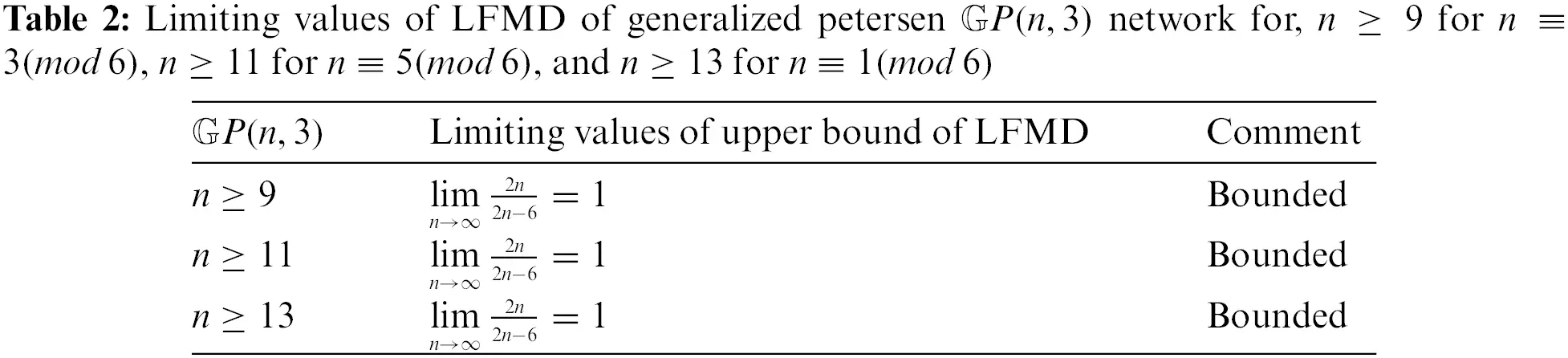
4 Discussion and Conclusion
In this paper, we have investigated the LFMD generalized Petersen network GP(n,3) for n≥7 with the exact value of lower and upper bounds. We have also checked the bounded and unbounded behavior of networks and found that for n≥8 and n≡0(mod2)GP(n,3) is bipartite Network having LFMD is 1. The details of computed values of LFMD are given in Tables 1 and 2. Even before the aforementioned tables, we illustrate Theorem 5 with the help of a example finding LFMD for the generalized Petersen graph with n=9. By Fig. 1b and Theorem 5 (Case A), it can be observed that the LRN sets of thee edges y1y4,y2y5,y3y6,y4y7,y5y8,y7y8,y8y2,y9y3 have the cardinality of 12 which is minimum among all the other LRNs. Moreover, the union of these LRNs is equal to the order of GP(n,3). The cardinality of the other LRNs with the intersection of this union is larger or equal to 12. By Theorem 1, dimlfGP(9,3)≤1812=32. In addition, the cardinality of LRNs with maximum cardinality is 18 consequently by Theorem 3, dimlfGP(9,3)≥1818=1. Therefore, 1≤dimlfGP(9,3)≤32.

Acknowledgement: The authors pay their sincerest thanks and deepest gratitude towards the referees for their valuable and precious comments that has helped us to soar up the manuscript to present level.
Funding Statement: The first author (Dalal Awadh Alrowali) was funded by the Deanship of Scientific Research at Jouf University under Grant No. DSR-2021-03-0301. The third author (Muhammad Javaid) is supported by the Higher Education Commission of Pakistan through the National Research Program for Universities Grant No. 20-16188/NRPU/R&D/HEC/2021 2021.
Conflicts of Interest: The authors declare that they have no conflicts of interest to report regarding the present study.
References
1. Harary, F., Melter, R. A. (1976). The metric dimension of a graph. Ars Combinatorica, 2(1), 191–195. [Google Scholar]
2. Khuller, S., Raghavachari, B., Rosenfeld, A. (1996). Landmarks in graphs. Discrete Applied Mathematics, 70(1), 217–229. DOI 10.1016/0166-218X(95)00106-2. [Google Scholar] [CrossRef]
3. Chvatal, V. (1983). Mastermind. Combinatorica, 3(1), 325–329. DOI 10.1007/BF02579188. [Google Scholar] [CrossRef]
4. Chartrand, G., Eroh, L., Oellermann, O. R. (2000). Resolvability in graphs and the metric dimension of a graph. Discrete Applied Mathematics, 105(1), 99–113. DOI 10.1016/S0166-218X(00)00198-0. [Google Scholar] [CrossRef]
5. Currie, J., Oellermann, O. R. (2001). The metric dimension and metric independence of a graph. Journal of Combinatorial Mathematics and Combinatorial Computing, 39(1), 157–167. [Google Scholar]
6. Beerliova, Z., Eberhard, F., Erlebach, T., Hall, A., Hoffman, M. et al. (2006). Network discovery and verification. IEEE Journal on Selected Areas in Communications, 24(1), 2168–2181. DOI 10.1109/JSAC.2006.884015. [Google Scholar] [CrossRef]
7. Fehr, M., Gosselin, S., Oellermann, O. R. (2006). The metric dimension of cayley digraphs. Discrete Mathematics, 306(1), 31–41. DOI 10.1016/j.disc.2005.09.015. [Google Scholar] [CrossRef]
8. Tomescu, I., Javaid, I. (2007). On the metric dimension of the jahangir graph. Bulletin Mathématique de la Société des Sciences Mathématiques de Roumanie, 50, 371–376. [Google Scholar]
9. Sebo, A., Tannier, E. (2004). On metric generators of graphs. Mathematics of Operations Research, 29(1), 383–393. DOI 10.1287/moor.1030.0070. [Google Scholar] [CrossRef]
10. Arumugam, S., Mathew, V. (2012). The fractional metric dimension of graphs. Discrete Mathematics, 312(1), 1584–1590. DOI 10.1016/j.disc.2011.05.039. [Google Scholar] [CrossRef]
11. Arumugam, S., Mathew, V. (2013). The fractional metric dimension of graphs. Discrete Mathematics, 5(1), 1–8. [Google Scholar]
12. Feng, M., Wang, K. (2013). On the metric dimension and fractional metric dimension of the hierarchical product of graphs. Applicable Analysis and Discrete Mathematics, 7(1), 302–313. DOI 10.2298/AADM130521009F. [Google Scholar] [CrossRef]
13. Feng, M., Kong, Q. (2018). On the fractional metric dimension of corona product graphs and lexicographic product graphs. Ars Combinatoria, 138, 249–260. [Google Scholar]
14. Saputro, S. W., Fenovcikova, A. S., Baca, M., Lascsakova, M. (2018). On fractional metric dimension of comb product graphs. Statistics, Optimization & Information Computing, 6, 150–158. [Google Scholar]
15. Yi, E. (2015). The fractional metric dimension of permutation graphs. Acta Mathematica Sinica, 31, 367–382. DOI 10.1007/s10114-015-4160-5. [Google Scholar] [CrossRef]
16. Liu, J. B., Kashif, A., Rashid, T., Javaid, M. (2019). Fractional metric dimension of generalized jahangir graph. Mathematics, 7, 1–10. DOI 10.3390/math7010100. [Google Scholar] [CrossRef]
17. Alkhaldi, A. H., Aslam, M. K., Javaid, M., Alanazi, A. M. (2021). Bounds of fractional metric dimension and applications with grid-related networks. Mathematics, 9, 2–18. DOI 10.3390/math9121383. [Google Scholar] [CrossRef]
18. Aisyah, S., Utoyo, M. I., Susilowati, L. (2019). On the local fractional metric dimension of corona product graphs, IOP conference series: Earth and environmental science. Hungarica, 243, 012043. DOI 10.1088/1755-1315/243/1/012043. [Google Scholar] [CrossRef]
19. Liu, J. B., Aslam, M. K., Javaid, M. (2020). Local fractional metric dimensions of rotationally symmetric and planar networks. IEE Access, 8, 82404–82420. DOI 10.1109/Access.6287639. [Google Scholar] [CrossRef]
20. Javaid, M., Zafar, H., Zhu, Q., Alanazi, A. M. (2021). Improved lower bound of LFMD with applications of prism-related networks. Mathematical Problems in Engineering, 2021, 9950310. DOI 10.1155/2021/9950310. [Google Scholar] [CrossRef]
21. Javaid, M., Raza, M., Kumam, P., Liu, J. B. (2020). Sharp bounds of local fractional metric dimensions of connected networks. IEE Access, 8(1), 172329–172342. DOI 10.1109/ACCESS.2020.3025018. [Google Scholar] [CrossRef]
22. West, D. B. (2000). Introduction to graph theory. 2nd edition. Prentice Hall, USA. [Google Scholar]
23. Ali, A., Chartrand, G., Zing, P. (2021). Irregularity in graphs. 1st edition. Springer. DOI 10.1007/978-3-030-67993-4. [Google Scholar] [CrossRef]

 Submit a Paper
 Propose a Special lssue
 Open Access
 View Full Text
 Download PDF
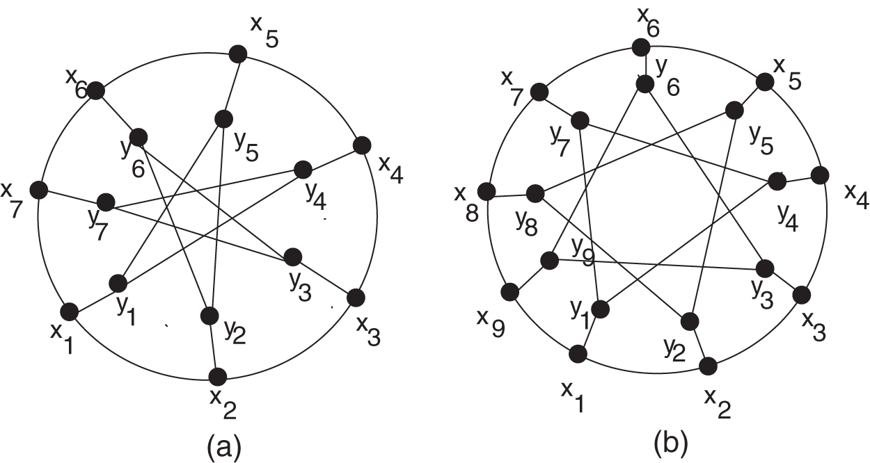

 Copyright © 2023 The Author(s). Published by Tech Science Press.
 Downloads
 Citation Tools