Brain Functional Networks with Dynamic Hypergraph Manifold Regularization for Classification of End-Stage Renal Disease Associated with Mild Cognitive Impairment

1  Introduction

In addition to renal failure, end-stage renal disease (ESRD) is usually accompanied by central nervous system abnormalities [1] and multiorgan dysfunction [2]. It may lead to cognitive dysfunction, including cognitive control abnormalities [3], memory impairment [4], and emotional impairment [5]. Cognitive impairment is a common comorbidity in ESRD cases [6], which may be caused by uremia, thiamine deficiency, hypertension, hemodialysis (HD), transplant rejection or electrolyte disorder. About 30%∼60% of ESRD patients will have cognitive impairment when receiving HD treatment [7]. Patients with mild cognitive impairment (MCI) have a higher risk of developing dementia, which may significantly reduce the odds of survival and prognosis [8]. The development of dementia in MCI patients may be delayed after certain cognitive training and rehabilitation treatment. Some patients can even return to a normal state, which not only relieves their own pain but also relieves the burden on family and society [9]. However, the exact neuropathological mechanism of ESRD associated with mild cognitive impairment (ESRDaMCI) remains unclear, hindering the development of effective treatment.

Nowadays, neuroimaging technology is developed in the detection and research of brain diseases, providing a valuable tool for the exploration of potential imaging biomarkers of ESRD-related neurological complications [10]. It allows us to effectively explore brains and their connectivity patterns in a noninvasive manner, revealing previously unrevealed aspects of brain function and brain structure. For example, previous voxel-based morphometrics, surface-based morphometrics, and diffusion tensor imaging studies have revealed defects in gray matter volume and reduced cortical thickness [11], as well as reduced white matter integrity [12] in ESRD patients. In addition, various analyses, including arterial spin labeling [13], magnetic resonance spectroscopy [14], and single-photon emission tomography [15], have found abnormalities in brain metabolism and function in ESRD patients treated with HD.

In recent years, resting-state functional magnetic resonance imaging (Rs-fMRI) has been attempted to detect changes in brain function behind neuropsychological injury in ESRD patients [16]. Brain functional networks (BFN) can describe the functional or structural interactions of the brain at the level of the whole brain connection [17], providing a new way to explore the function and structure of the brain. BFN construction and analysis are generally applied to early diagnosis and prediction of brain diseases. Previous Rs-fMRI studies [16] have shown that patients with ESRD show internal abnormalities in brain activity, with disruption of functional connectivity networks within and between regions, especially in certain key brain regions. In the context of cognitive decline in ESRD patients, changes in the global brain functional network have not been fully understood. In Rs-fMRI studies, BFN is generally constructed from a full time series of resting states. Studies have shown that the neural activity of the brain changes dynamically over time, and such dynamic changes will contain richer information [18]. This study of dynamic BFN (DBFN) helps to further explore the operation mode of the whole brain, which is conducive to the auxiliary diagnosis of brain diseases.

Manifold regularization (MR) has been widely used in constructing BFN. Li et al. [19] were inspired by the similar connection mode (internal similar structure) between adjacent brain regions in BFN, expanded MR by embedding sparse prior information, and obtained a BFN construction method called sparse MR (SMR). Xue et al. [20] constructed a BFN based on the same idea and introduced the distance information between brain regions into the manifold regular term. Most BFN construction methods only consider the paired association between brain regions, but ignore the higher-order relationship between multiple brain regions. Studies have shown that in BFN, a brain region usually interacts directly with several adjacent brain regions. Thus, higher-order relationships between brain regions may contain important information to improve classification performance. Zhou et al. [21] proposed a hypergraph-based learning method which introduced a hypergraph Laplacian operator to describe the higher-order relations between multiple samples. Yu et al. [22] adopted hypergraphs to depict higher-order relationships between multiple nodes and applied them in the study of BFN. Jie et al. [23] used sparse representation (SR) to form hypergraph, directly carried out feature extraction and feature selection in the diagnosis of MCI. Ji et al. [24] developed a manifold regularization term on the basis of hypergraph, and constructed a DBFN with hypergraph manifold regularization regularization (HMR) for MCI classification.

The relationship between nodes in most of the above models comes from the attributes of the data itself, which is a static relationship. If only the initial hypergraph structure is used and the dynamic modification of the hypergraph structure by the adjusted feature embedding is ignored, the model will ignore many implicit relationships that are not included in these static relationships. Recent studies have shown that the structure and function of brain networks are altered in ESRD patients [25,26]. Nevertheless, they did not focus on the topological organization features of the whole brain functional network in ESRDaMCI patients. To solve these problems, we proposed a DBFN construction method based on dynamic hypergraph manifold regularization (DHMR), and applied it to the classification of ESRDaMCI patients and normal people. Firstly, the optimization model of DBFN is constructed. Secondly, the dynamic hypergraph is constructed based on DBFN. Then, the DHMR and L1 norm regularization were introduced into the optimization model to obtain a DBFN (DDBFN) constructed based on DHMR method. Finally, the constructed DDBFN is used for the diagnosis and prediction of ESRDaMCI to verify the validity of the proposed method.

2  Data and Methods

2.1 Research Framework

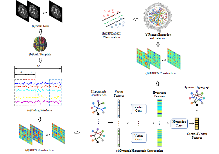
Fig. 1 shows our research framework, including the following steps: (a) Preprocessing the original resting state fMRI data obtained by scanning; (b) Registering preprocessed fMRI data to different brain regions according to the standard partition template to obtain the time series of all brain regions; (c) Dividing the whole time series into multiple overlapping subseries segments by the sliding windows; (d) Constructing a DBFN based on PC and converting it into an optimization model; (e) Forming hypergraphs based on DBFN, extracting features from the constructed hypergraphs by convolution operation, and forming new hypergraphs to obtain their Laplacian matrix; (f) Constructing the manifold regular terms using hypergraph Laplacian matrix, and introducing the manifold regular terms and sparse regular terms into the PC-based optimization model to obtain a DDBFN; (g) Extracting the network edge weights in DDBFN as features, and using t-test to select features to obtain discriminant features; (h) Training a linear kernel SVM classifier by the training set, and classifying the test sets and evaluating the classification performance.

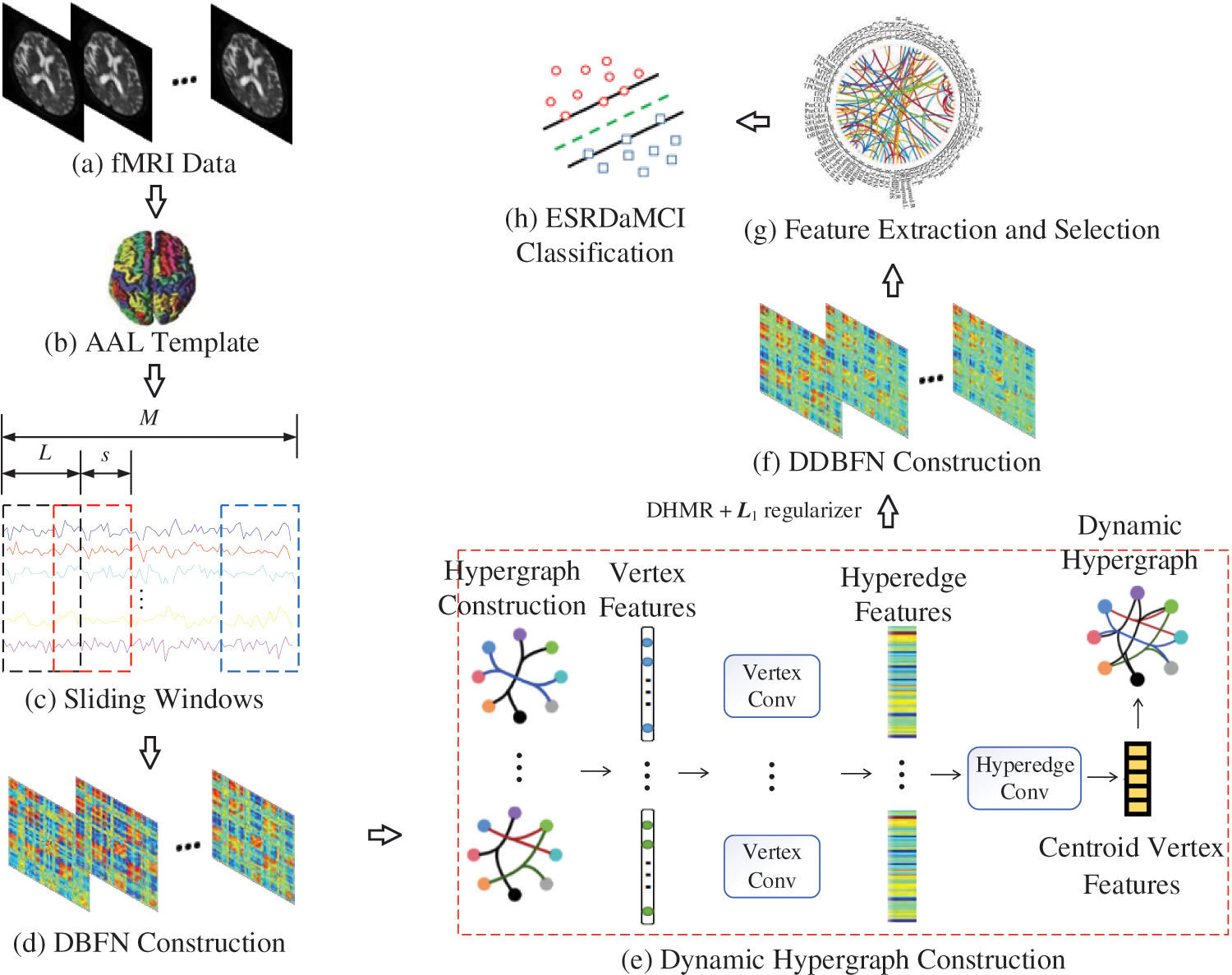
Figure 1: Research framework diagram

2.2 Data Acquisition and Processing

Fifty-one patients with ESRD who had been diagnosed with MCI (ESRDaMCI group) were included in the study. They were admitted to Changzhou Second People’s Hospital affiliated to Nanjing Medical University from February 2020 to June 2021. All of them were right-handed and had no previous cardiovascular disease. No neurological diseases; No infectious diseases; No diabetes mellitus; No contraindications for MRI examination. Besides, thirty-nine healthy volunteers (normal group) were recruited, all were right-handed; Previous good health; No contraindications for MRI examination. In the ESRDaMCI group and the normal group, five and three subjects were excluded due to excessive head movement, respectively. Finally, fifty-one patients and thirty-nine volunteers were included. This study was approved and supervised by the Ethics Committee of Changzhou Second People’s Hospital affiliated to Nanjing Medical University with the approval number KY039-01. All subjects voluntarily signed a written informed consent.

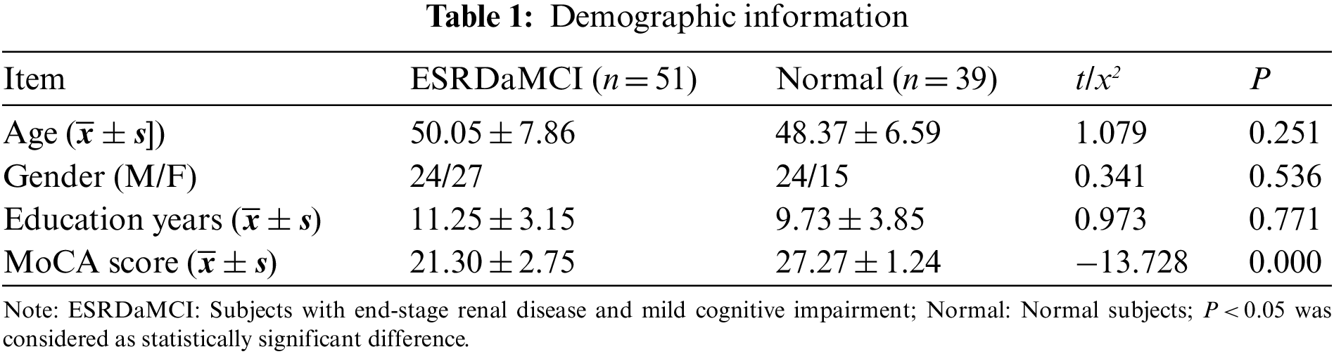
Montreal cognitive assessment scale (MoCA) is a tool for assessing cognitive abnormalities. It consists of eleven items, which are used to measure various cognitive domains. Such as memory, language, abstract thinking, executive function, visual-spatial skills, attention and concentration, calculation, and orientation. According to the statistics of Changzhou Second People’s Hospital Affiliated with Nanjing Medical University, MoCA was better completed and is more sensitive to identifying MCI in the memory clinic than other cognitive function assessment scales, considering such factors as patients’ temper and uncooperation [27]. Therefore, the cognitive functions of these ESRD patients were evaluated by MoCA. The full score of MoCA scale was 30, with 26 or more being normal, 18–26 being mild, 10–17 being moderate, and less than 10 being severe. All neuropsychological tests were evaluated by a neurologist with 20 years of experience prior to the MRI scan. The average score of ESRD subjects diagnosed with MCI was 21.30 ± 2.75. Table 1 shows the specific demographic information.

We used GE Discovery MR 750W 3.0 T superconducting MR scanner with 32 channel head and neck joint coils. Soft rubber plugs were used to fix the head to avoid artifacts caused by subjects’ head movement in the test. All subjects underwent routine MR examinations, including T2-weighted (T2WI), fluid-attenuated inversion recovery (FLAIR) sequence T2WI, and two imaging physicians ruled out organic craniocranial lesions. Gradient echo plane echo imaging (GRE-EPI) sequence to collect Rs-fMRI images, machine scanning parameters: Repetition time (TR) is 2000 ms, echo time (TE) is 40 ms, field of view (FOV) is 24 cm, flip angle (FA) is 90°, and matrix size is 64 × 64. The layer thickness is 6 mm. MoCA assessment was completed prior to scanning.

After obtaining Rs-fMRI data of patients and normal subjects, Data Processing Assistant for Resting-state fMRI (DPARSF) based on Matlab 2012b platform was used to preprocess the original data [28]. Preprocessing operations need to install beforehand SPM8 toolkit (http://www.fil.ion.ucl.ac.uk/spm/) and DPARSF toolkit (http://rfmri.org/dparsf). The specific steps are as follows: (a) Format conversion: Convert the Rs-fMRI data from DICOM format to NIFTI format using DICOM import of SPM8; (b) Slice timing: Delete the first ten time points of each subject, and use the remaining 230 time series for subsequent processing (since it takes a certain amount of time for both the instrument and the subject to enter the stable state); (c) Realign and normalize: Perform head correction using rigid registration, and congruence fMRI images to Montreal Neurological Institute (MNI) space, followed by standardized operations (Bounding Box: [−90,−126,−72; Voxel Size: [333]); (d) Space smoothing: Smooth the Gaussian kernel with full-width-at-half-maximum; (e) Detrend; (f) Band pass filtering: Set the frequency range from 0.01 to 0.08 Hz; (g) Regions partition: Partition each subject’s brain into 90 regions according to Automated Anatomical Labeling (AAL) standard template [29] and extract the time series of each brain region for subsequent research after the removal of covariates.

2.3 Dynamic Hypergraph

BFN was constructed using pairwise Pearson’s correlation coefficients (PCC) between brain pairs. We think of brain regions as nodes and PCC as the edges connecting them. PCC is calculated using the following method:

pij=corr{x(i),x(j)}(1)

where x(i) and x(j) represent the i-th and j-th brain regions, respectively, and corr is the pinional correlation coefficient of x(i) and x(j).

Sliding windows [30] were adopted to divide the entire Rs-fMRI time series into several subsequences to obtain a DBFN. Assume that the total number of time points of Rs-fMRI is M, D = [(M-L)/s]+1 is the number of subsequences that can be generated, X=[x1,x2,…,xp]∈RM×P is the matrix composed of time series, where L is the length of sliding window, s is the step length, and P is the number of brain regions. The time series of d-th window in i-th brain region was defined as xid∈RL(d=1,…,D), and the time series matrix of d-th window was obtained by connecting xid in series:

X(d)=[x1d,x2d,…,xpd]∈RL×P(2)

PCC between time series in each time window is calculated and a DBFN is constructed.

After the centralization and standardization of xid, the correlation coefficient matrix of the d-th window can be expressed as Z(d)≈(X(d))TX(d), which can be converted into the optimized form:

minZ(d)||Z(d)−X(d)TX(d)||F2(3)

For a given time series X, a hypergraph G(V, E, W) network can be used to describe the attribute relationships between brain regions. The set of nodes is represented as V, the set of hyperedges is represented as E, and the set of weights of each hyperedge is represented as W. In hypergraph G, each brain region corresponds to a node v∈V in the hypergraph, and each hyperedge contains more than two nodes to represent the simultaneous interaction of multiple brain regions.

Assume that H∈R|V|×|E| is the point-edge association matrix of the hypergraph G, where the values of matrix elements are defined as follows:

h(v,e)={1,v∈e0,v∉e(4)

where v∈V is a node of hypergraph G, and e∈E is a hyperedge of hypergraph G.

For an association matrix H, the node degree d(vi) of each node and the edge degree δ(ei) of each hyperedge are respectively expressed as:

d(vi)=∑ei∈Ew(ei)h(vi,ei),i=1,…,m(5)

δ(ei)=∑vi∈Vh(vi,ei),i=1,…,m(6)

where ei (i = 1,… , m; m is the number of hyperedges) is the i-th hyperedge, w(ei) is the weight of the hyperedge, and vi is the i-th node.

The DBFN is constructed based on sliding windows, that is, a complete time series is divided into several equal length window segments, and then the brain network matrix of each segment is calculated. Finally, these continuous brain network matrices form a dynamic brain network. Although constructing the DBFN is dynamic for the whole time series, the method of constructing the BFN on each window fragment is still static for each window fragment [31]. In other words, the relationship between traditional hypergraph nodes comes from the attributes of the data itself, which is a static relationship. Only the initial hypergraph structure is used, while the dynamic modification of the hypergraph structure by the adjusted feature embedding is ignored. This may cause the model to ignore many implicit relationships that are not included in these static relationships [32].

To obtain a dynamic hypergraph, the method of node convolution and hyperedge convolution superposition [32] is adopted to dynamically modify the structure of the hypergraph. First, node convolution is performed to aggregate node features to the hyperedge containing these nodes. The transformation matrix T is learned from the node features to replace and weight the node features in the hyperedge, the multilayer perceptron (MLP) is used to generate the transformation matrix T. Then we use the one-dimensional convolution to compress the transformed features:

T=MLP(Xu)xe=conv(T⋅MLP(Xu))(7)

where Xu represents the node feature set, xe represents the adjacent hyperedge feature.

Then, hyperedge convolution is performed to aggregate hyperedge features into centroid node features. Use MLP to generate the weight score of each super edge. The output centroid node features are calculated as the weighted sum of the input hyperedge features.

w∗=softmax(xeB+b)(8)

xu=∑i=0|A(u)|w∗ixei(9)

where w* is the weight of each super edge, B and b are learnable parameters, xu represents centroid node characteristics, and |A(u)| represents the size of the adjacent super edge set.

Node features are updated to embed new features, and a new hypergraph structure is constructed on this basis by combining with node convolution and hyperedge convolution. Table 2 shows the algorithm of dynamic hypergraph construction.

We initialize the hypergraph structure by embedding the input features. With the enhancement of feature embedding degree and the deepening of network embedding degree, the hyperedge set is also dynamically adjusted, so that a better hypergraph structure can be obtained. Finally, a new dynamic hypergraph G*(V*, E*, W*) is obtained.

2.4 DBFN Based on DHMR

Laplacian matrix can reflect the intrinsic geometric structure of a graph, so it is often used in the matrix representation of graph. The Laplacian matrix of a hypergraph can better reflect higher-order relations between nodes, which can be expressed as

L=Dv−Θ(10)

where Θ=HWDe−1HT is the adjacency matrix of the hypergraph, Dv is the node degree matrix with the diagonal element d(vi), De is the hyperedge degree matrix with the diagonal element δ(ei).

The standardized Laplacian matrix of the dynamic hypergraph is deduced and calculated according to the calculation method of Laplacian matrix of a simple graph, as shown in Eq. (11):

Ldh=I−Dv∗−12H∗W∗De−1H∗TDv∗−12(11)

where Ldh is the normalized Laplacian matrix of the dynamic hypergraph, and I is the identity matrix. Dv* is the node degree matrix of the dynamic hypergraph, De* is the hyperedge degree matrix of the dynamic hypergraph, W* is the diagonal matrix in which the diagonal elements are the weights of each hyperedge of the dynamic hypergraph, and H∗∈R|V∗|×|E∗| is the point-edge correlation matrix of the hypergraph G*.

Referring to the method of Shao et al.’s [33], a common k-nearest neighbor (KNN) algorithm is used to construct dynamic hypergraphs on the basis of DBFN, and popular regularization terms and L1 norm regularization terms are added to calculate the node degree and edge degree of dynamic hypergraphs, thus obtaining the regular terms of hypergraphs. Inspired by Jiang et al. [32] and Ji et al. [24], we added a hypergraph convolution method based on node convolution and hyperedge convolution superposition to dynamically update the hypergraph structure and obtained a new DBFN construction method, namely, DHMR. The objective function of this method is shown in Eq. (12):

minZ(d)||Z(d)−X(d)TX(d)||F2+λ||Z(d)||1+βtr(Z(d)TLdhZ(d))(12)

where X(d) represents the time series matrix of the d-th window, λ and β represent the regularization parameters of L1 norm regularization term and manifold regularization term, respectively, and Ldh is the normalized Laplacian matrix of the dynamic hypergraph.

The diagonal value of the DDBFN matrix finally obtained was changed to zero to make our method comparable with other methods. That is, the self-connection of the two regions was not calculated in this study.

2.5 Feature Extraction, Selection and Classification

After obtaining BFN of all subjects, the next task was to classify ESRDaMCI and normal subjects according to the estimated BFN. The problem then turns to determining which features [34] should be used for classification. In BFN analysis, two methods are commonly used to identify cognitive impairment. One is to extract features based on some graph measures, such as local clustering coefficients [35,36]. The other is to directly take network edge weights as features [37]. We adopted the second method, which can reduce the influence of different extracted features on the validation of BFN itself. The simplest t-test method is used to select features to avoid the confounding effect of feature extraction.

Support vector machine (SVM) has good generalization performance [38] and uses a kernel function to map samples to high-dimensional space during classification. It can simplify linear separable problems in high-dimensional space. Linear kernel SVM is easy to employ and easy to compare experimental results, and has been widely used in small-sample classification problems [39]. The t-test method selects features with discriminating ability, and uses the selected features to train SVM for recognition. The optimization objective function of SVM classifier can be expressed as

L(w,β,a)=∑p=1nap−12∑p,q=1nypyqapaqK⟨xp,xq⟩s.t.K⟨xp,xq⟩=xpTxqw=∑p=1lapypxp,∑p=1lapyp=00≤ap≤C,p=1,…,n(13)

where K⟨xp, xq⟩ is a linear kernel function, yp ∈ {−1, +1} represents the label, n is the training sample, and ap is the training parameter.

3  Experiment and Analysis

Due to the limited number of samples, the leave-one-out cross-validation (LOOCV) was adopted to evaluate the performance of the proposed method [40]. In simple terms, one is tried on the test, and the others are tried on the training model. The training set cannot participate in the testing process of the model, because such participation would result in information disclosure and artificially improve the performance of the model. We can unify the information of the brain region relationship and feature embedding relationship by constructing the dynamic hypergraph and then constructing the DDBFN. We firstly discuss the effects of different parameters on the classification performance of ESRDaMCI, and determine the optimal parameters of the proposed method, and then uses six different relevant approaches to construct DBFN for comparison, to evaluate the performance of the proposed method.

3.1 Parameter Selection

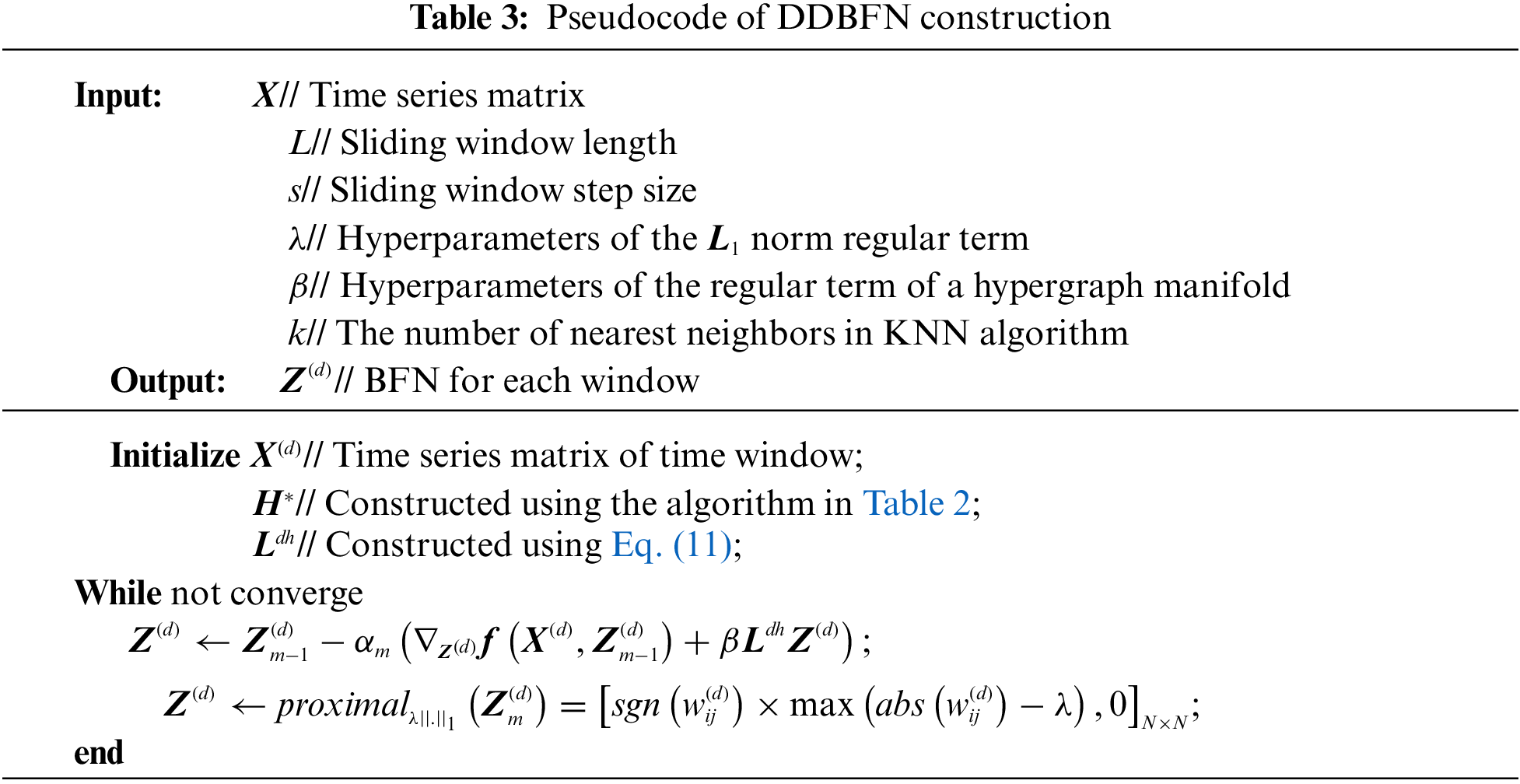
We set ten step sizes, s = 1, 2,… , 10, and ten sliding window lengths, L = 10, 20, …, 100. The nearest neighbor number k is 1, 3, 5, 6, 7, 8, 9, 10, and 15 [33]. The regularization parameters λ and β are in the range of {2−4, 2−3, 2−2, 2−1}. The significance level of t-test feature selection was set to 0.05, and the linear kernel classifier parameter C of SVM was set to one. Proximal operator method [19] is used to optimize and solve the L1 norm regularization terms, as shown in Table 3. Z(d) is updated m times using gradient descent, and αm is the step size in gradient descent. Then the nearest neighbor operator of the L1 norm regular term is calculated to apply soft threshold operation to the elements in Z(d). After each gradient descent calculation is completed, the proximal operator method is used to calculate the nearest neighbor operator of Z(d), which is updated in the next iteration. Thus, when the objective function converges, the optimal solution of Z(d), namely, DDBFN, is obtained.

Because of multiple parameters, the grid search method cannot find the optimal parameters directly. Our strategy is to work out the optimal parameters separately, that is, work out the optimal parameters step by step. In this study, the LOOCV method was adopted to gradually obtain the optimal parameter values of the model, that is, the window size and step size were determined according to DBFN first, and then the nearest neighbor number and regularization parameters were determined. The ESRDaMCI patient training set was used to find the optimal classification model and the test set was used to evaluate the model. In this way, the number of classifiers and test results corresponding to the sample size are obtained. The average of the test results is then calculated to measure the performance of the model. To avoid data leakage, the optimal hyperparameter is determined by a repeated training model, and the optimal hyperparameter model is verified by the original samples.

Classification accuracy (ACC), area under ROC curve (AUC), sensitivity (SEN), and specificity (SPE) were used to evaluate classification performance [41]. ACC is defined as the ratio of the number of correctly predicted tags to the number of the entire sample. The AUC measures the probability that the classifier will rank a randomly selected positive sample higher than a randomly selected negative sample. SEN and SPE are called true positive rate and false positive rate, respectively.

The length L and step s of the sliding window are important parameters of DDBFN analysis, which will greatly affect the reliability of DDBFN. Since DDBFN was optimized by DBFN, we first classified all DBFN of the subjects based on different L and s to determine the optimal L and s. In the classification, patients were treated as positive samples and normal subjects as negative samples. The classification performance with multiple groups of parameters was analyzed to determine the optimal L and s. For each window length, each index value and standard deviation of the group with higher classification performance are shown in Table 4, where the best classification results are highlighted in black bold.

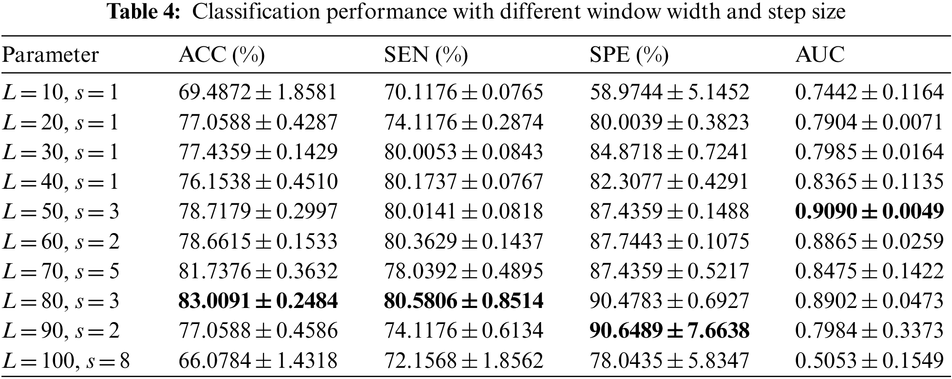
It can be seen from Table 4 that the classification effect is best when L is set to 80 and s is set to 3. The classification performance first gets better and then gets worse with the increase of L and s. Accordingly, the appropriate window length and step size should be selected, which is consistent with the conclusion in the study of Li et al. [41]. The reason may be that the information is too dense with the small window length, which makes the classification performance not very good. Large window size and large step size may lead to the loss of some dynamic information between brain regions over time, resulting in the decline of classification performance, while moderate window size and large step size correspond to considerable classification performance.

After determining the window size and step size, we determine the optimal neighbor number k and regularization parameters λ and β. KNN algorithm is used to select k nodes closest to the central node to form a hyperedge, so different neighbor numbers have a great impact on the classification performance. L1 regular term is mainly to remove redundant features and make DDBFN sparser. The regular term of a hypergraph manifold preserves the discriminant information of each subject and induces more discriminant features. In general, the regularization parameters λ and β are also important to regulate the complexity of constructing DBFN. Regularization parameters with better classification performance under each neighbor number k are shown in Table 5, by comparing the values of various classification indexes with different regularization parameters under the same k, where k = 1 means that no hypergraph is formed.

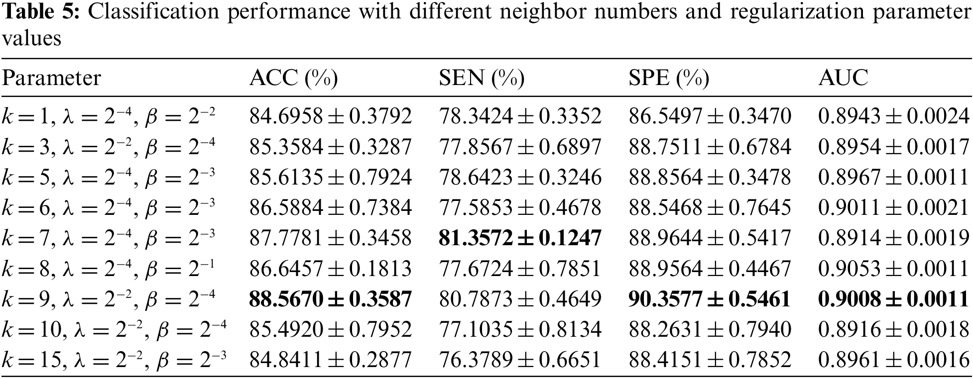
It can be seen from Table 5 that ACC, SPE, and AUC are the best when k = 9, and the error range is small, which is generally consistent with the research conclusion of Shao et al. [33]. The classification performance increases first and then decreases when the value of k changes from small to large. The possible reason is that when k is small, it depicts too many features. When the value of k is large, the hypergraph describes the overall structural features of BFN rather than local features. Many nodes on the edge may belong to different categories, so it is difficult to reflect the structural features of BFN well. It can be found that k = 9, λ = 2−2, β = 2−4 have the best classification performance. To sum up, we set the window length as 80, step size as 3, nearest neighbor number as 9, regularization parameters λ = 2−2 and β = 2−4 to construct DDBFN.

3.2 DBFN Construction

Several different BFN construction methods, including PC [19], SR [19], MR [19], SMR [19], HMR [24], and SHMR [24] (the nearest neighbor number corresponding to the optimal classification performance is 7), were used to construct DBFN, and these comparison methods were all relevant to the proposed method. Feature selection was carried out by t-test with a significance level of 0.05, and linear kernel SVM classifier was adopted to complete classification. Their classification performance for ESRDaMCI is shown in Table 6, where the optimal classification result is indicated in bold.

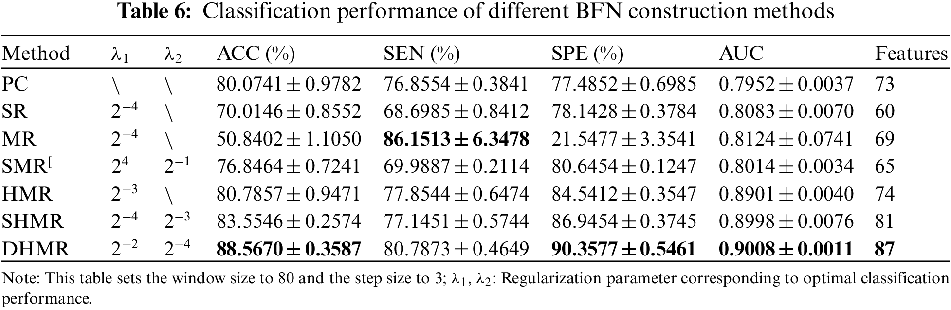
Fig. 2 visualizes the classification performance of different BFN construction methods. It can be seen intuitively that DHMR method has better classification performance for ESRDaMCI than six related methods except for SEN, thus achieving the best classification effect. The best ACC, SPE, and AUC are 88.5670% ± 0.3587%, 90.3577% ± 0.5461% and 0.9008 ± 0.0011, respectively. Compared with other methods, the error range of the proposed method is smaller, and the average of the selected features in LOOCV is the largest. It indicates that DBFN constructed by our method is more stable and may contain more potential information. The average ACC, SEN, SPE, and AUC of the SHMR method were 5.0124%, 3.6422%, 3.4123%, and 0.001 higher than those of the SHMR method, and six more than those of the SHMR method.

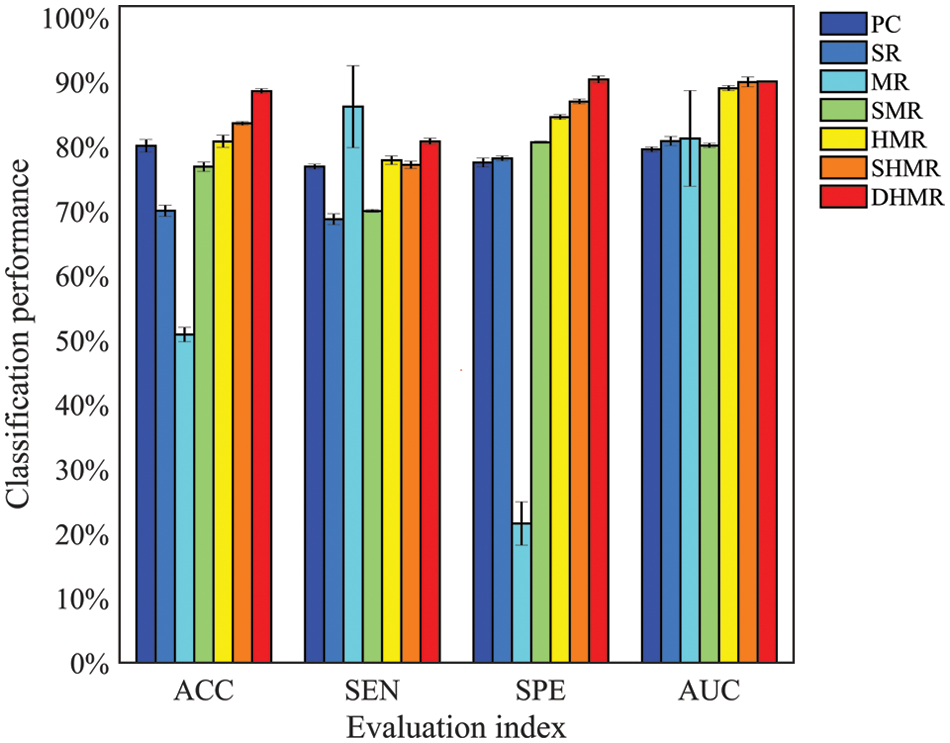
Figure 2: Visualization of classification performance

As can be seen from Fig. 2, the classification performance of SR is better than MR, that of SMR is better than SR, and that of HMR is better than SMR. This indicates that introducing L1 norm regularization and streamlining regularization on the basis of the SR method can effectively improve the quality of DBFN and increase the classification accuracy. Conversely, introducing only L1 norm regularization cannot improve the classification performance. These are consistent with the research conclusions of Li et al. [41]. The classification performances of the HMR method and SHMR method are better than those of the PC method, which proves the effectiveness of introducing the regular term of hypergraph manifold. The DHMR method is slightly better than SHMR, which also shows the effectiveness of dynamic hypergraph in BFN.

In essence, we focus only on the node-based functional connection approach, using network matrices to visualize the constructed BFN. An ESRDaMCI subject was randomly selected to visualize BFN of the same subject in the same time window after constructing DBFNs using our method and the other six methods. The results are shown in Fig. 3.

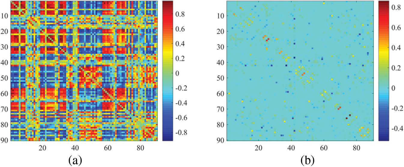
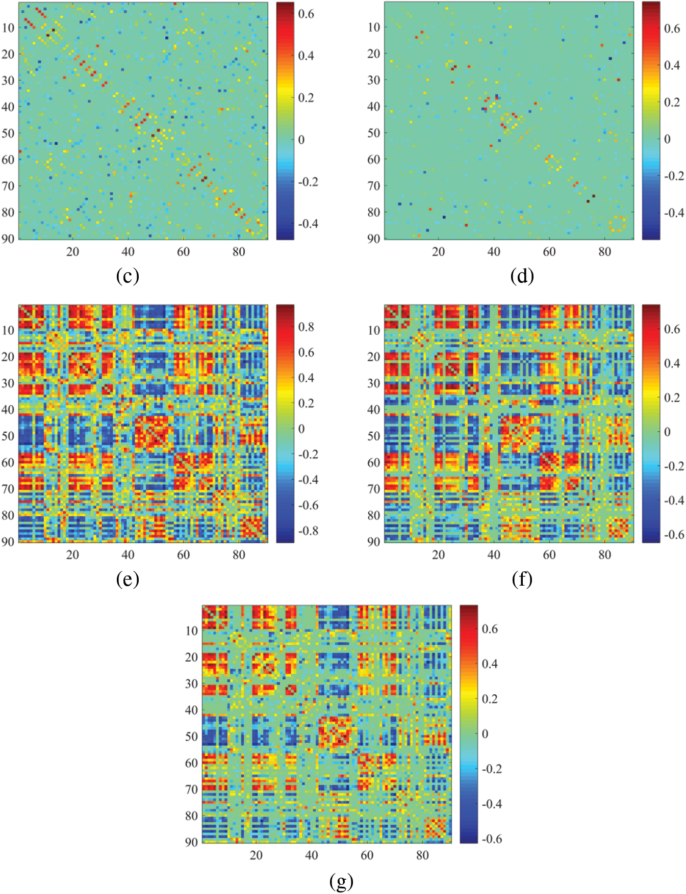
Figure 3: Visualization results of BFN in the same time window. (a) PC, (b) SR, (c) MR, (d) SMR, (e) HMR, (f) SHMR, (g) DHMR

It can be observed in Fig. 3 that the topologies of BFN with the same time window formed by PC and SR are quite different. The BFN of the same time window constructed based on PC tends to be dense, while the BFN of the same time window constructed based on SR is sparse, because they use different data fitting terms. We note that the traditional data deletion scheme has a significant impact on the network structure, but our proposed DHMR method can preserve the original network structure well. It weakens some possible noisy connections and makes the BFN matrix clearer, while maintaining the original sparse structure. Fig. 3g is sparser and has a clearer topology than Figs. 3a, 3e, 3f.

3.3 Discriminative Regions

We used connections in BFN to identify features from patients with ESRDaMCI. The main question, therefore, is which features contribute to the final classification. DDBFN was constructed based on the optimal classification performance to find some biomarkers for ESRDaMCI diagnosis. Then the features (i.e., network “connections”) were sorted by p-values to obtain 87 features with p-value less than 0.05 and high frequency in LOOCV. We also counted the features with a high frequency of each functional subnetwork in the cross validation, and finally obtained the 87 discriminating features involved in the classification task. They were visualized, as shown in Fig. 4.

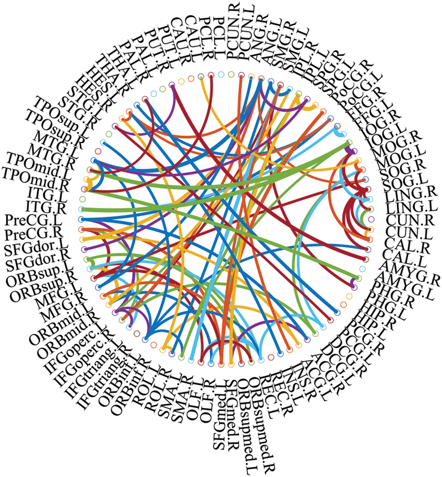
Figure 4: The most discriminating features (network connections)

In Fig. 4, the thickness of each arc is inversely proportional to the corresponding p-value, indicating the distinguishing ability of the corresponding feature (not its actual connectivity strength). The color of each arc is randomly assigned, just for better visualization. From the connections in Fig. 4, we found that the brain regions associated with the 87 most discriminating features mainly included 21 brain regions, such as the left middle temporal gyrus (MTG.L), right amygdala (AMYG.R), left superior marginal gyrus (SMG.L) and right hippocampus (HIP.R), which were called discriminative regions, as shown in Table 7. These findings are consistent with previous pathological studies of MCI and neuroimaging biomarkers [42,43], and are largely consistent with brain regions with significant differences in topological properties between the two groups of subjects studied by Wu et al. [44].

It can be seen from Table 7, the selected discriminative regions are mainly located in the left brain, which is considered for logical task processing, language, and analytical thinking. For example, left orbitofrontal superior frontal gyrus (ORBsup.L), left middle frontal gyrus (MFG.L), left insular inferior frontal gyrus (IFGoperc.L), left orbitofrontal inferior frontal gyrus (ORBinf.L) [45] are mainly related to creative and advanced mental activities such as thinking and consciousness. The right hippocampus (HIP.R) [46] plays an important role in short-term memory, long-term memory, and spatial localization. Right amygdala (AMYG.R) [47] mainly affects motivation, emotional control, fear, and interpretation of the nonverbal emotional expression. The occipital lobe includes the left superior occipital gyrus (SOG.L), left middle occipital gyrus (MOG.L), left inferior occipital gyrus (IOG.L), and right inferior occipital gyrus (IOG.R) [48], which are responsible for vision, image recognition and image perception. The middle left transverse temporal gyrus (HES.L), left middle temporal gyrus (MTG.L) and right temporal pole: middle temporal gyrus (TPOmid.R) [47] are closely related to short-term memory, balance and emotional, if these brain regions damage can lead to the change of personality. These brain regions were selected to indicate that ESRDaMCI subjects had changes in memory, language, spatial and visual processing, etc., compared with normal subjects.

Some selected discriminative regions, including the right hippocampus (HIP.R), left parietal and inferior angular gyrus (IPL.L), and left angular gyrus (ANG.L), belong to default mode network (DMN), and are related to memory, sensation, and visual language, respectively. DMN plays an important role in cognitive function and neuromodulation. Although the results of our experiment revealed that only three brain regions of ESRDaMCI subjects’ brain function changes were located in DMN, the specific DMN regions were different. The results indicate that our study may provide the most discriminating features and discriminative regions leading to ESRDaMCI, providing a reference for clinical diagnosis.

3.4 Refine and Differentiate the Degree of Cognitive Impairment

Bai et al. [49] found that some topological attributes of nodes with significant differences could be considered as neuroimaging biomarkers to evaluate the degree of ESRD associated with cognitive impairment. Hence, we analyzed the topological attributes of the discriminative regions in the two types of functional subnetworks, including degree, betweenness centrality, local efficiency, clustering coefficient, small-world attribute and shortest path length. Since the preprocessed Rs-fMRI data spans 230 time points, the length of a sliding window was 80 and the step size was 3, so each subject had 51 functional subnetworks. The specific steps are to extract the degree, intermediate centrality, local efficiency, clustering coefficient, small-world attribute, and shortest path length of the functional subnetworks, respectively. Then calculate the average value, respectively, and extract the topological attributes of discriminative regions, respectively. As a result, we can obtain the node topological attributes of discriminative regions of the two types of subjects. Independent sample t-test was used to compare the topological attributes of discriminative regions between the two groups, and p < 0.05 was considered as statistically significant. Table 8 shows the average topological properties of discriminative regions.

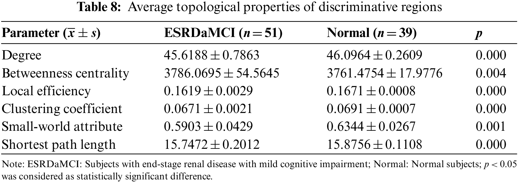
As can be seen from Table 8, the p-values of the average topological attributes of the discriminative regions of the two groups of subjects are all less than 0.05. Degree, betweenness centrality, local efficiency, clustering coefficient, small-world attribute, and shortest path length are statistically significant, which also proves the accuracy of the discriminative regions we selected for ESRDaMCI. Sequently, the degree, local efficiency, and clustering coefficient with p-values less than 0.001 were selected as neuroimaging biomarkers to evaluate the degree of cognitive impairment of ESRDaMCI. Degree, local efficiency, and clustering coefficient of discriminative regions are shown in Fig. 5, where the first 51 numbers belong to ESRDaMCI group and the last 39 belong to normal group.

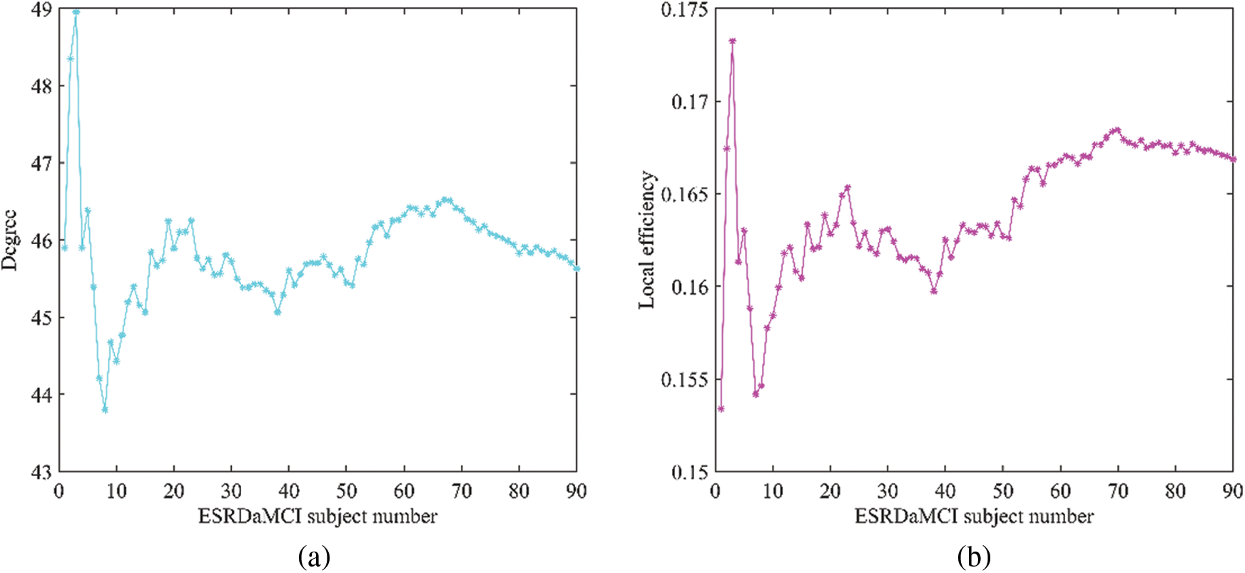
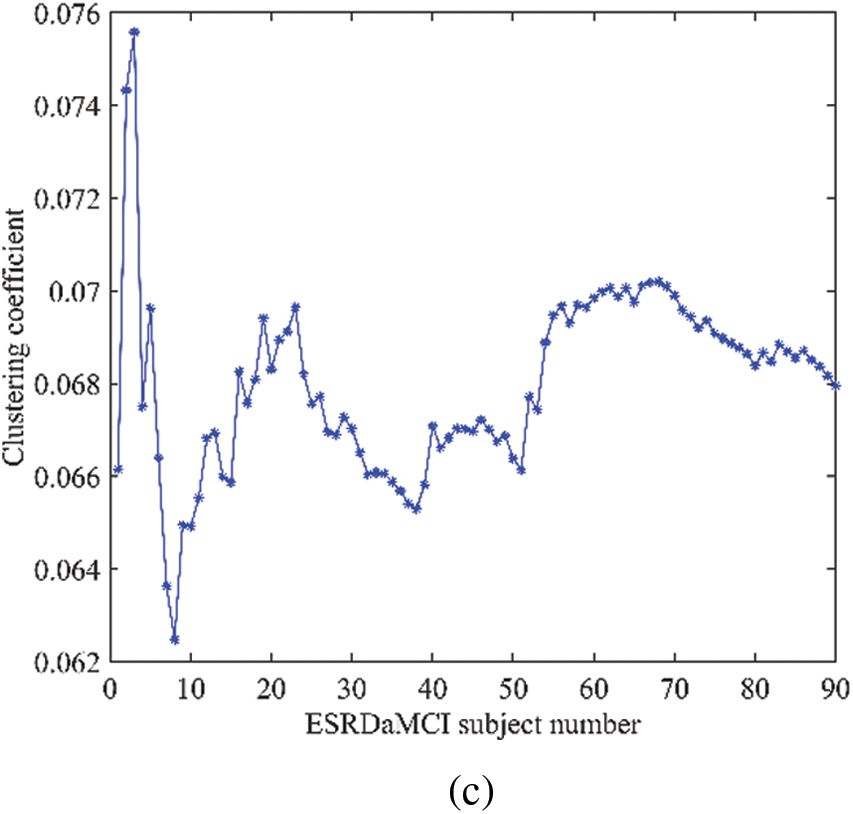
Figure 5: Topological attributes of discriminative regions (a) degree, (b) local efficiency, (c) clustering coefficient values

As can be seen from Fig. 5, the degree, local efficiency, and clustering coefficient of ESRDaMCI subjects are mostly lower than those of normal subjects. Among them, the values of the two subjects are higher than those of normal subjects, indicating that ESRD might be mixed in ESRDaMCI subjects without cognitive impairment. The possible reason is that the previous MoCA scale score is not very accurate. Multi-objective optimization [50,51] is adopted to rank 51 ESRDaMCI subjects according to degree, local efficiency, and clustering coefficient. The ESRDaMCI subjects are clustered to further refine and distinguish the cognitive impairment degree of ESRDaMCI subjects. The degree of cognitive impairment is defined as 0∼1, and the closer it is to 1. The higher the degree of cognitive impairment is. Fig. 6 shows the order of cognitive impairment degree of all subjects.

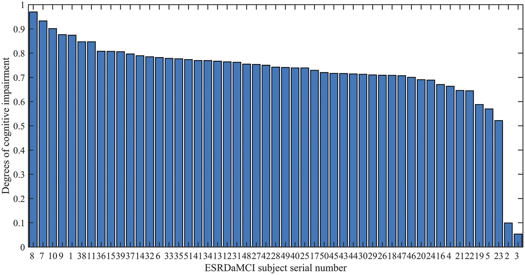
Figure 6: Ranking of cognitive impairment degree of ESRDaMCI subjects

As can be seen from Fig. 6, the degrees of cognitive impairment of ESRDaMCI subjects are significantly different from left to right. The specific classification is as follows: subjects 8, 7, 10, 9, 1, 38, and 11 have higher degrees of cognitive impairment, while subjects 19, 5, and 23 have lower degrees of cognitive impairment. Subjects 2 and 3 may be with ESRD but without cognitive impairment, while the other subjects suffer from moderate cognitive impairment. It indicates that the degrees of cognitive impairment are different in MCI patients. The possible reason is that MCI can further subdivide the degree of cognitive impairment, and the MoCA scale is limited, which cannot refine and distinguish the degrees of cognitive impairment in MCI patients. The degree of cognitive impairment in ESRDaMCI subjects is subdivided according to node topological attributes of the discriminative regions, providing a reference for clinical diagnosis.

4  Discussion

In recent years, there has been an increasing interest in epidemiology, clinical features, neuroimaging, biomarkers, disease mechanisms, neuropathology, and clinical trials of diseases associated with MCI. The threshold for such comorbidities remains a challenge, whereas these challenges may turn into opportunities to further explore the human brain with the development of new neuroimaging techniques and new research methods. Thus, there are relatively few studies on the classification of ESRDaMCI. Most studies are based on the attributes of the data themselves, and only consider the paired relationship between two brain regions. They do not take into account the non-negligible dynamic high-order relationship between the functional connections of multiple brain regions, which is also an important prior information.

At present, relevant studies have modeled the high-order relationship between multiple brain regions. For example, Chen et al. [52] introduced “correlation’s correlation” to construct high-order functional networks, and then employed the k-means clustering method to reduce the dimensionality of high-order functional networks, and verified the effectiveness of this method in MCI classification experiments. Zhou et al. [53] proposed a high-order functional network construction method based on the normal distribution of matrix variables. The DBFN of each subject was taken as samples and assumed to follow the normal distribution of matrix variables. These methods have some drawbacks. Chen et al.’s [52] method involving many parameters is easy to overfit in classification with limited training data, but it is not supported by a mathematical model. Zhou et al.’s [53] require strict assumptions so that subsequent conclusions can be established. Therefore, it is essential to describe the complex relationship between brain regions. In this study, node features in particular are updated to embed new features, and a new hypergraph structure is constructed on this basis. Many vertices are on the same hyperedge, so dynamic hypergraphs can well reflect this higher-order relation and make reasonable explanations. Compared with general networks, this model has high-order and dynamic characteristics and provides more feature information.

It is worth mentioning that Jie et al. [23] directly carried out feature extraction, feature selection, and classification of the formed a hypergraph. The relationship between nodes comes from the attributes of the data itself, which is a static relationship. This can cause the model to ignore many implicit relationships that are not included in these static relationships. After obtaining the hypergraph in DBFN based on PC, node convolution and hyperedge convolution superposition are adopted to dynamically modify the hypergraph structure to obtain the dynamic hypergraph, and then its node degree and edge degree are calculated to obtain the manifold regular term of the dynamic hypergraph and introduce it into BFN construction. The constructed BFN can simultaneously capture the dynamic correlations and complex high-order relationships between brain regions. Jie et al. only focused on high-order relationships between multiple brain regions in their study.

However, the proposed method also needs some improvement. Firstly, the KNN method is not interpretable in the field of neuroimaging, and the SR method [23] can be used to form hypergraphs in future work. Secondly, the simplest t-test and SVM are used for feature selection and classification. In the future, feature selection can be improved by iterating feature selection in the training set combined with the test set to gradually select the features which can improve the classification performance. SVM can also be optimized using the whale algorithm and other methods to optimize the classifier.

5  Conclusion

In summary, we proposed a DBFN construction method based on DHMR and applied it to the classification of ESRDaMCI. This method considers the higher-order characteristics of BFN and the richer information provided by DBFN. It extends the MR method, makes DBFN more biologically significant, and can effectively improve the classification performance of DBFN with ESRDaMCI. Firstly, a dynamic high-order BFN is constructed, a t-test is used to select the effective features, and SVM is used to classify the network features. Among the seven comparable BFN construction methods, this method achieves the best classification result. Furthermore, we also identified discriminative regions based on the selected features to better reflect the pathogenesis of ESRDaMCI, and refined and differentiated the cognitive impairment degree of ESRDaMCI subjects through the node topology attributes of discriminative regions.

Nevertheless, there are some limitations in our work. First of all, we did not consider biological mechanisms. The experiment was purely data-driven. Second, we only used single mode imaging (Rs-fMRI), and the data should be collected in a larger database. Next, we classified normal subjects and ESRDaMCI subjects and only considered the dichotomous problem. To break through these limitations, we will introduce multimodal imaging and more training samples to potentially improve classification accuracy. In addition, we will establish multiclassification tasks, such as adding ESRD subjects without cognitive impairment to form a three-classification problem, to verify our method more comprehensively.

Funding Statement: Our work was supported by the National Natural Science Foundation of China (No. 51877013), (ZJ), (http://www.nsfc.gov.cn/), the Jiangsu Provincial Key Research and Development Program (No. BE2021636), (ZJ), (http://kxjst.jiangsu.gov.cn/), and the Science and Technology Project of Changzhou City (No. CE20205056), (ZJ), (http://kjj.changzhou.gov.cn/). This work was also sponsored by Qing Lan Project of Jiangsu Province (no specific grant number), (ZJ), (http://jyt.jiangsu.gov.cn/).

Conflicts of Interest: The authors declare that they have no conflicts of interest to report regarding the present study.

References

1. de Deyn, P. P., Saxena, V. K., Abts, H., Borggreve, F., D’Hooge, R. et al. (1992). Clinical and pathophysiological aspects of neurological complications in renal failure. Acta Neurologica Belgica, 92(4), 191–206. [Google Scholar]
2. Li, S. M., Ma, X. F., Huang, R. W., Li, M., Tian, J. Z. et al. (2016). Abnormal degree centrality in neurologically asymptomatic patients with end-stage renal disease: A resting-state fMRI study. Clinical Neurophysiology: Official Journal of the International Federation of Clinical Neurophysiology, 127(1), 602–609. DOI 10.1016/j.clinph.2015.06.022. [Google Scholar] [CrossRef]
3. Tamura, M. K., Yaffe, K. (2011). Dementia and cognitive impairment in ESRD: Diagnostic and therapeutic strategies. Kidney International, 79(1), 14–22. DOI 10.1038/ki.2010.336. [Google Scholar] [CrossRef]
4. Ma, X. F., Jiang, G. H., Li, S. M., Wang, J. H., Zhan, W. F. et al. (2015). Aberrant functional connectome in neurologically asymptomatic patients with end-stage renal disease. PLoS One, 10(3), e0121085. DOI 10.1371/journal.pone.0121085. [Google Scholar] [CrossRef]
5. Chilcot, J., Wellsted, D., da Silva-Gane, M., Farrington, K. (2008). Depression on dialysis. Nephron Clinical Practice, 108(4), C256–C264. DOI 10.1159/000124749. [Google Scholar] [CrossRef]
6. Brouns, R., de Deyn, P. P. (2004). Neurological complications in renal failure: A review. Clinical Neurology and Neurosurgery, 107(1), 1–16. DOI 10.1016/j.clineuro.2004.07.012. [Google Scholar] [CrossRef]
7. Tyler, H. R. (1965). Neurological complications of dialysis, transplantation, and other forms of treatment in chronic uremia. Neurology, 15(12), 1081. DOI 10.1212/WNL.15.12.1081. [Google Scholar] [CrossRef]
8. Raphael, K. L., Guo, W., Greene, T., Baird, B. C., Beddhu, S. (2012). Cognitive function and the risk of death in chronic kidney disease. American Journal of Nephrology, 35(1), 49–57. DOI 10.1159/000334872. [Google Scholar] [CrossRef]
9. Wang, S. H., Zhang, Y. D., Li, Y. J., Jia, W. J., Liu, F. Y. et al. (2018). Single slice based detection for Alzheimer’s disease via wavelet entropy and multilayer perceptron trained by biogeography-based optimization. Multimedia Tools and Applications, 77(9), 10393–10417. DOI 10.1007/s11042-016-4222-4. [Google Scholar] [CrossRef]
10. Zhang, Y. D., Dong, Z. C., Wang, S. H., Yu, X., Gorriz, J. M. et al. (2020). Advances in multimodal data fusion in neuroimaging: Overview, challenges, and novel orientation. Information Fusion, 64, 149–187. DOI 10.1016/j.inffus.2020.07.006. [Google Scholar] [CrossRef]
11. Dong, J. W., Ma, X. F., Lin, W. H., Liu, M. C., Fu, S. S. et al. (2018). Aberrant cortical thickness in neurologically asymptomatic patients with end-stage renal disease. Neuropsychiatric Disease and Treatment, 14, 1929–1939. DOI 10.2147/NDT. [Google Scholar] [CrossRef]
12. Drew, D. A., Koo, B. B., Bhadelia, R., Weiner, D. E., Duncan, S. et al. (2017). White matter damage in maintenance hemodialysis patients: A diffusion tensor imaging study. BMC Nephrology, 18(1), 213. DOI 10.1186/s12882-017-0628-0. [Google Scholar] [CrossRef]
13. Jiang, X. L., Wen, J. Q., Zhang, L. J., Zheng, G., Li, X. et al. (2016). Cerebral blood flow changes in hemodialysis and peritoneal dialysis patients: An arterial-spin labeling MR imaging. Metabolic Brain Disease, 31(4), 929–936. DOI 10.1007/s11011-016-9829-7. [Google Scholar] [CrossRef]
14. Zhang, C. Y., Chen, Y., Chen, S., Kong, X. C., Liu, Y. et al. (2017). Evaluation of mental disorders using proton magnetic resonance spectroscopy in dialysis and predialysis patients. Kidney & Blood Pressure Research, 42(4), 686–696. DOI 10.1159/000484023. [Google Scholar] [CrossRef]
15. Polinder-Bos, H. A., Elting, J., Aries, M. J., García, D. V., Willemsen, A. T. et al. (2018). Changes in cerebral oxygenation and cerebral blood flow during hemodialysis-A simultaneous near-infrared spectroscopy and positron emission tomography study. Journal of Cerebral Blood Flow & Metabolism, 40(2), 328–340. DOI 10.1177/0271678X18818652. [Google Scholar] [CrossRef]
16. Peng, C., Luo, T. Y., Yang, H. (2019). Immediate abnormal intrinsic brain activity patterns in patients with end-stage renal disease during a single dialysis session: A resting-state functional MR imaging study. Proceedings of the 17th National Academic Conference of Medical Imaging Committee of Chinese Association of Integrated Traditional and Western Medicine, the 6th Annual Academic Conference of Medical Imaging Committee of Gansu Association of Integrated Traditional and Western Medicine, Lanzhou, China. [Google Scholar]
17. Jiao, Z. Q., Ji, Y. X., Zhang, J. H., Shi, H. F., Wang, C. (2020). Constructing dynamic functional networks via weighted regularization and tensor low-rank approximation for early mild cognitive impairment classification. Frontiers in Cell and Developmental Biology, 8, 610569. DOI 10.3389/fcell.2020.610569. [Google Scholar] [CrossRef]
18. Chang, C., Glover, G. H. (2010). Time–frequency dynamics of resting-state brain connectivity measured with fMRI. NeuroImage, 50(1), 81–98. DOI 10.1016/j.neuroimage.2009.12.011. [Google Scholar] [CrossRef]
19. Li, W. K., Xu, X. W., Jiang, W., Wang, P. J., Gao, X. (2020). Functional connectivity network estimation with an inter-similarity prior for mild cognitive impairment classification. Aging, 12(17), 17328–17342. DOI 10.18632/aging.103719. [Google Scholar] [CrossRef]
20. Xue, Y. F., Zhang, L. M., Qiao, L. S., Shen, D. G. (2020). Estimating sparse functional brain networks with spatial constraints for MCI identification. PLos One, 15(7), e0235039. DOI 10.1371/journal.pone.0235039. [Google Scholar] [CrossRef]
21. Zhou, D., Huang, J., Scholkopf, B. (2007). Learning with hypergraphs: Clustering, classification, and embedding. Proceedings of the 19th International Conference on Neural Information Processing Systems, pp. 1601–1608. Vancouver, British Columbia, Canada. [Google Scholar]
22. Yu, J., Rui, Y., Tang, Y. Y., Tao, D. (2014). High-order distance-based multi-view stochastic learning in image classification. IEEE Transactions on Cybernetics, 44(12), 2431–2442. DOI 10.1109/TCYB.2014.2307862. [Google Scholar] [CrossRef]
23. Jie, B., Wee, C. Y., Shen, D. G., Zhang, D. Q. (2016). Hyper-connectivity of functional networks for brain disease diagnosis. Medical Image Analysis, 84–100. DOI 10.1016/j.media.2016.03.003. [Google Scholar] [CrossRef]
24. Ji, Y. X., Zhang, Y. T., Shi, H. F., Jiao, Z. Q., Wang, S. H. et al. (2021). Constructing dynamic brain functional networks via hyper-graph manifold regularization for mild cognitive impairment classification. Frontiers in Neuroscience, 15, 669345. DOI 10.3389/fnins.2021.669345. [Google Scholar] [CrossRef]
25. Jin, M., Wang, L. Y., Wang, H., Han, X., Diao, Z. L. et al. (2021). Altered resting-state functional networks in patients with hemodialysis: A graph-theoretical based study. Brain Imaging and Behavior, 15(2), DOI 10.1007/s11682-020-00293-8. [Google Scholar] [CrossRef]
26. Park, B. S., Si, E. K., Lee, H. J., Yang, W. K., Kang, M. P. (2020). Alterations in structural and functional connectivities in patients with end-stage renal disease. Journal of Clinical Neurology, 16(3), 390–400. DOI 10.3988/jcn.2020.16.3.390. [Google Scholar] [CrossRef]
27. Xu, C. Y., Chen, C. C., Guo, Q. W., Lin, Y. W., Meng, X. Y. et al. (2021). Comparison of moCA-B and MES scales for the recognition of amnestic mild cognitive impairment. Journal of Alzheimer’s Disease and Related Disorders, 4(1), 33–36. [Google Scholar]
28. Rubinov, M., Sporns, O. (2010). Complex network measures of brain connectivity: Uses and interpretations. Neuroimage, 52, 1059–1069. DOI 10.1016/j.neuroimage.2009.10.003. [Google Scholar] [CrossRef]
29. Tzourio-Mazoyer, N., Landeau, B., Papathanassiou, D., Crivello, F., Etard, O. et al. (2002). Automated anatomical labeling of activations in SPM using a macroscopic anatomical parcellation of the MNI MRI single-subject brain. Neuroimage, 15(1), 273–289. DOI 10.1006/nimg.2001.0978. [Google Scholar] [CrossRef]
30. Lei, B. Y., Yu, S. Z., Zhao, X., Frangi, A. F., Tan, E. L. et al. (2020). Diagnosis of early Alzheimer’s disease based on dynamic high order networks. Brain Imaging and Behavior, 15(1), 276–287. DOI 10.1007/s11682-019-00255-9. [Google Scholar] [CrossRef]
31. Huang, J. S., Dai, B., Ding, W. P., Zhang, D. Q. (2021). Brain network analysis and its application. Data Acquisition and Processing, 36(4), 648–663. [Google Scholar]
32. Jiang, J., Wei, Y., Feng, Y. (2019). Dynamic hypergraph neural networks. International Joint Conferences on Artifical Intelligence (IJCAI), pp. 2635–2641. DOI 10.24963/ijcai.2019/366. [Google Scholar] [CrossRef]
33. Shao, W., Peng, Y., Zu, C., Wang, M. L., Zhang, D. Q. (2019). Hypergraph based multi-task feature selection for multimodal classification of Alzheimer’s disease. Computerized Medical Imaging and Graphics, 80, 101663. DOI 10.1016/j.compmedimag.2019.101663. [Google Scholar] [CrossRef]
34. Li, H. J., Wang, Z., Pei, J., Cao, J., Shi, Y. (2020). Optimal estimation of low-rank factors via feature level data fusion of multiplex signal systems. IEEE Transactions on Knowledge and Data Engineering, 34(6), 2860–2871. DOI 10.1109/TKDE.2020.3015914. [Google Scholar] [CrossRef]
35. Mahajan, S., Pandit, A. K. (2021). Hybrid method to supervise feature selection using signal processing and complex algebra techniques. Multimedia Tools and Applications. DOI 10.1007/s11042-021-11474-y. [Google Scholar] [CrossRef]
36. Li, H. J., Bu, Z., Wang, Z., Cao, J. (2019). Dynamical clustering in electronic commerce systems via optimization and leadership expansion. IEEE Transactions on Industrial Informatics, 16(8), 5327–5334. DOI 10.1109/TII.9424. [Google Scholar] [CrossRef]
37. Shuai, H., Jing, L., Liang, S., Ye, J., Fleisher, A. et al. (2010). Learning brain connectivity of Alzheimer’s disease by sparse inverse covariance estimation. Neuroimage, 50(3), 935–949. DOI 10.1016/j.neuroimage.2009.12.120. [Google Scholar] [CrossRef]
38. Wang, S. H., Nayak, D. R., Guttery, D. S., Zhang, X., Zhang, Y. D. (2021). COVID-19 classification by CCSHNet with deep fusion using transfer learning and discriminant correlation analysis. Information Fusion, 68, 131–148. DOI 10.1016/j.inffus.2020.11.005. [Google Scholar] [CrossRef]
39. Bi, X. A., Xie, Y., Wu, H., Xu, L. Y. (2021). Identification of differential brain regions in MCI progression via clustering-evolutionary weighted SVM ensemble algorithm. Frontiers of Computer Science, 15(6), 156903. DOI 10.1007/s11704-020-9520-3. [Google Scholar] [CrossRef]
40. Jiao, Z. Q., Xia, Z. W., Ming, X. L., Cheng, C., Wang, S. H. (2019). Multi-scale feature combination of brain functional network for eMCI classification. IEEE Access, 7(1), 74263–74273. DOI 10.1109/Access.6287639. [Google Scholar] [CrossRef]
41. Li, Y., Liu, J. Y., Gao, X. Q., Jie, B., Kim, M. et al. (2018). Multimodal hyper-connectivity of functional networks using functionally-weighted LASSO for MCI classification. Medical Image Analysis, 52(10), 80–96. [Google Scholar]
42. Mckhann, G., Chertkow, H., Hyman, B. T. (2011). The diagnosis of dementia due to Alzheimer’s disease: Recommendations from the national institute on aging-Alzheimer’s association workgroups on diagnostic guidelines for Alzheimer’s disease. Alzheimers Dement, 7(3), 263–269. DOI 10.1016/j.jalz.2011.03.005. [Google Scholar] [CrossRef]
43. Greicius, M. (2008). Resting-state functional connectivity in neuropsychiatric disorders. Current Opinion in Neurology, 21(4), 424–430. DOI 10.1097/WCO.0b013e328306f2c5. [Google Scholar] [CrossRef]
44. Wu, B. L., Yue, Z., Li, X. K., Li, L., Zhang, M. et al. (2020). Brain functional network changes in patients with end-stage renal disease and its correlation with cognitive function. Chinese Journal of Neuromedicine, 19(2), 181–187. [Google Scholar]
45. Zhang, Y. D., Wang, S. H., Phillips, P., Yang, J., Yuan, T. F. (2016). Three-dimensional eigenbrain for the detection of subjects and brain regions related with Alzheimer’s disease. Journal of Alzheimer’s Disease, 50(4), 1163–1179. DOI 10.3233/JAD-150988. [Google Scholar] [CrossRef]
46. Wang, S. H., Zhang, Y. D., Liu, G., Phillips, P., Yuan, T. F. (2016). Detection of Alzheimer’s disease by three-dimensional displacement field estimation in structural magnetic resonance imaging. Journal of Alzheimer’s Disease, 50(1), 233–248. DOI 10.3233/JAD-150848. [Google Scholar] [CrossRef]
47. Zhang, Y. D., Dong, Z. C., Phillips, P., Wang, S. H., Ji, G. L. et al. (2015). Detection of subjects and brain regions related to Alzheimer’s disease using 3D MRI scans based on eigen brain and machine learning. Frontiers in Computational Neuroscience, 9, 66. [Google Scholar]
48. Wang, S. H., Du, S., Zhang, Y., Phillips, P., Wu, L. N. et al. (2017). Alzheimer’s disease detection by pseudo zernike moment and linear regression classification. CNS & Neurological Disorders Drug Targets, 16(1), 11–15. DOI 10.2174/1871527315666161111123024. [Google Scholar] [CrossRef]
49. Bai, Z. G. (2016). Changes of brain function and DTI in patients with renal failure. Guangzhou, China: Southern Medical University. [Google Scholar]
50. Zhang, Y. D., Wang, S. H., Sui, Y. X., Yang, M., Liu, B. et al. (2018). Multivariate approach for Alzheimer’s disease detection using stationary wavelet entropy and predator-prey particle swarm optimization. Journal of Alzheimer’s Disease, 65(3), 855–869. DOI 10.3233/JAD-170069. [Google Scholar] [CrossRef]
51. Mahajan, S., Abualigah, L., Pandit, A. K., Altalhi, M. (2022). Hybrid aquila optimizer with arithmetic optimization algorithm for global optimization tasks. Soft Computing, 26, 4863–4881. DOI 10.1007/s00500-022-06873-8. [Google Scholar] [CrossRef]
52. Chen, X. B., Zhang, H., Lee, S. W., Shen, D. G. (2017). Hierarchical high-order functional connectivity networks and selective feature fusion for MCI classification. Neuroinformatics, 15, 271–284. DOI 10.1007/s12021-016-9321-x. [Google Scholar] [CrossRef]
53. Zhou, Y. Y., Qiao, L. S., Li, W. K., Zhang, L. M., Shen, D. G. (2018). Simultaneous estimation of lo-and high-order functional connectivity for identifying mild cognitive impairment. Frontiers in Neuroinformatics, 12(3), 1–8. DOI 10.3389/fninf.2018.00003. [Google Scholar] [CrossRef]
Cite This Article
Copyright © 2023 The Author(s). Published by Tech Science Press.
This work is licensed under a Creative Commons Attribution 4.0 International License , which permits unrestricted use, distribution, and reproduction in any medium, provided the original work is properly cited.
Downloads
Citation Tools