Remote Sensing Data Processing Process Scheduling Based on Reinforcement Learning in Cloud Environment

1  Introduction

With the advancement of remote sensing technology and the successful launch of various remote sensing satellites, remote sensing data has grown exponentially. Various remote sensing data processing methods emerge [1–3], and processing remote sensing data via remote sensing technology with cloud computing has become one of the most dazzling areas [4]. Since most remote sensing data are time-sensitive, making use of these remote sensing data has become necessary in the era of big data. At the same time, workflow technology is often introduced to form a remote sensing data processing process to deal with the management and control of the production process of remote sensing products.

Usually, the remote sensing data processing needs to perform multi-level segmentation on the distributed data divided by remote sensing image spatial blocks in cloud storage and adopt appropriate scheduling strategies. It usually has problems like considerable update delay and low access efficiency of remote data. Efficient scheduling algorithms are essential for remote sensing data processing systems. Task scheduling is a Non-deterministic Polynomial Complete problem in process processing, and the scheduling performance directly affects the performance of the remote sensing data processing system [5]. Remote sensing data processing is carried out in a cluster environment, and there is no suitable scheduling algorithm in the remote sensing data processing computing platform [6].

Heuristic methods are commonly used to solve scheduling problems at present, such as Heterogeneous Earliest Completion Time (HEFT) [7], Min-min [8], Max-min [9], Particle Swarm Optimization (PSO) [10], and Genetic Algorithm (GA) [11], etc. The application of Min-min and Max-min as greedy strategies can easily cause load imbalance; HEFT cannot effectively solve the large and complicated remote sensing data processing process. The standard PSO and GA methods easily fall into the local optimum solution. A learning-based method [12–14] could be used to improve the efficiency and effectiveness of cloud resource management. Besides, Reinforcement Learning (RL) is a popular learning method for improving resource utilization. Q-learning [15,16] can be used to explore the optimal solution for the scheduling problem. Due to the defect of the Q-value matrix dimension explosion, it has a high algorithm storage complexity. DQN uses value function approximation to solve the problem of Q-learning. For high-dimensional data storage problems, a fixed-dimensional environment state vector and a single type of workflow are used to train a reinforcement learning model. Still, its model generalization ability has limitations. This paper proposes a policy gradient method WDRL with a baseline to solve scheduling problem of the remote sensing data processing flow. This method improves upon Richard Sutton’s REINFORCE [17] approach for task scheduling. The optimal order of learning and selecting agent tasks is provided according to the matching degree of neural network computing tasks and resources. It then learns from experience through a trajectory-driven simulation to optimize the overall completion time of the processing flow and improve resource utilization.

The datasets used for this paper include remote sensing data workflow for water surface temperature inversion [18–20] and scientific workflow SIPHT for bioinformatics [21–23], which are of a more significant practical reference value. At the same time, traditional scheduling methods such as Heterogeneous Earliest Completion Time (HEFT), Min-min, Max-min, etc., which are more integrated types of algorithms in current commercial systems, are used to test the data, and then this study compares the results. It is proved that the algorithm proposed in this paper has a good optimization performance.

The WDRL proposed in this paper has the following contributions to the remote sensing data processing flow. First, the scheduling problem with the constraint of minimizing makespan of the remote sensing data processing flow is transformed into a continuous decision process, and a markov decision process is used to model it; second, the state space and the action space of the markov decision process problem are defined; the input parameter model, neural network model [24] and minimized time reward function are designed; third, proposes a dynamic workflow scheduling method based on deep reinforcement learning and real-world workflow templates. Many case studies have been carried out to verify the effectiveness of our method.

2  Problem Analysis

A scientific workflow is represented by a Directed Acyclic Graph (DAG) W = (T, E), as shown in Fig. 1, where T = {t1, t2,…,tn} is a set of n tasks, and E is a set of priority dependencies. Each task ti represents a single application with runtime at some task instance; the priority dependency eij = (ti, tj) indicates that tj starts after the task node ti receives data; the starting point of the dependency ei and the endpoints are called parent and child tasks, respectively. Workflows start and end by entering and exiting tasks, respectively. In a cloud environment, a task must be mapped to a set of resources that serve as a set of Virtual Machines (VMs) to execute a task; this set represents VM = {vm0, vm1,…,vmm}. Each virtual machine has a corresponding capacity {CPU, memory, bandwidth}.

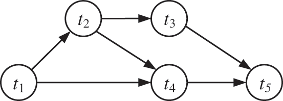
Figure 1: A workflow example with 5 tasks

Cloud computing provides an on-demand service model with available, convenient, and on-demand access to a configurable computing resource pool. It consists of networks, servers, memory, application software, services, and other resources, as shown in Fig. 2. Based on different levels of service provision, three cloud service models have been proposed, namely Infrastructure as a Service (IaaS), Platform as a Service (PaaS), and Software as a Service (SaaS). Simulation of the IaaS cloud is used as a support platform for workflows in the study. Cloud application service providers lease cloud resource nodes in virtual machines from IaaS service providers, and tasks submitted by users are scheduled to virtual machines with good fitness by the task scheduler. The physical host is transparent to users/the user. These virtual machines are heterogeneous in hardware and software facilities such as CPU, memory, operating system, etc., to handle different tasks. At the same time, virtual machines may exist in various geographical distributed data centres, and their power consumption, electricity price, and network delay vary.

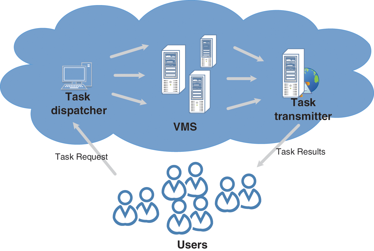
Figure 2: Cloud computing model

3  Background

Consider the general setup shown in Fig. 3, an agent interacts with the environment. At each step t, the agent observes state St and is asked to choose an action. After executing the action, the state of the environment is transferred to St + 1, and the agent simultaneously obtains the reward Rt. State transitions and rewards are random and assumed to have Markov properties; that is, the probability and rewards of state transitions depend only on the state St of the environment and the actions taken by the agent.

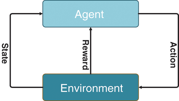
Figure 3: Markov decision model

The learning goal is to maximize the expected cumulative reward. An agent can only control his behaviour, without knowing what state the environment will transform into, nor what the rewards will be. Therefore, the agent can observe these quantities during the training process by interacting with the environment.

There are many forms of approximators to choose. In recent years, deep neural networks have been successfully applied as an approximator to many large-scale reinforcement learning problems. We adopt a fully connected neural network as the brain and train its learnable parameters using policy gradients. Deep neural networks (DNNs) [24] have been successfully used as function approximators to solve large-scale RL tasks recently. An advantage of DNNs is that they do not require manual configuration of features. Inspired by these successes, we use neural networks to represent policies in our design. Let J(θ) be the expectation of cumulative reward and τ be the trajectory experienced by an individual during an event. We have the following formula:

J(θ)=Eτ∼πθ(τ)[r(τ)](1)

πθ(τ)=v(s1)πθ(a1∣s1)∏t=2Tπ(st∣st−1,at−1)πθ(at∣st)(2)

∇θJ(θ)=∫πθ(τ)∇θlog⁡πθ(τ)r(τ)dτ(3)

π(at∣st) represents the agent, given a state st, what action the actor will take at will depend on the actor’s parameters θ. As the actions of the actors are different, each of the same trajectory will have a different probability of appearance; π(st∣st−1,at−1) stands for the environment.

The direction of the probability that the trajectory increases is the gradient term ∇θlog⁡πθ(τ), which is multiplied by the reward r to raise the trajectory to a higher total reward in a single round with a higher probability of appearance. Since the strategy does not generate deterministic actions, the same strategy will generate different trajectories in multiple rounds. To avoid serious deviation, it is necessary to improve the accuracy by sampling multiple times and taking the average. The gradient calculation is shown as follows:

∇θJ(θ)≈1N∑i=1N[(∑t=1Tlogπθ(ai,t∣si,t))(∑t=1Tr(si,t,ai,t))](4)

The main idea of the policy gradient method is to estimate the gradient by observing the trajectory of the policy execution. In a simple Monte Carlo method [25], the agent samples multiple trajectories and uses the empirically computed cumulative discounted reward as an unbiased estimate of the policy. Then the policy parameters are updated by gradient ascent.

θ←θ+α∑t∇θlogθ⁡(st,at)rt(5)

where α is the step size. This equation is obtained from REINFORCE algorithm [17], which is intuitively understood as: towards the direction ∑t∇θlog⁡πθ(st,at) gives how to change the policy parameters to increase πθ(st,at) (the action of the state probability); the basic framework flow of the algorithm is shown in Fig. 4.

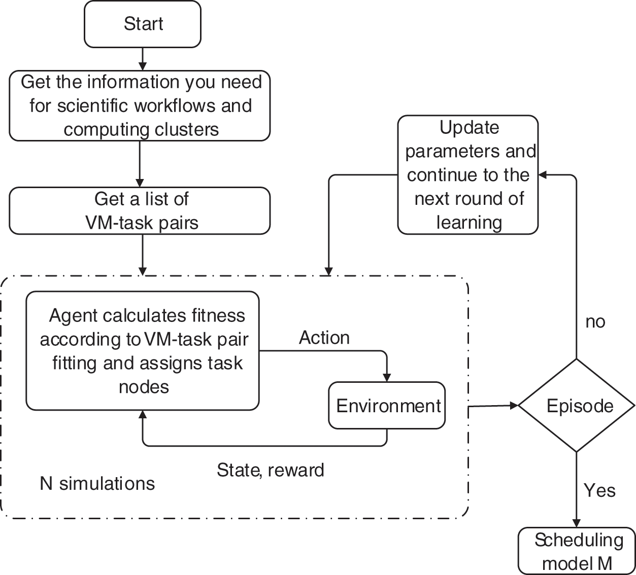
Figure 4: The basic flow chart of the algorithm

4  Algorithm Design

4.1 Algorithm

4.1.1 State Space

In WDRL, we use the allocation state of an available resource to determine the state of the environment rather than just representing it by the state of the current task. The state of the whole system is represented by a list of virtual-machines and tasks. Before each assignment, the agent will get a list of available resources that can be matched.

4.1.2 Rewards

One of the most important steps in reinforcement learning solutions is the design of rewards. It informs the actor that in a given state, certain actions are encouraged, while others are discouraged, and even others are punished. After repeated attempts, we gave a negative reward to ensure the effectiveness of learning. Throughout the testing process, in order to optimize the objective function, the agent will maximize the cumulative reward value. The reward is given at the end of a full schedule.

4.1.3 Action Space

In the cluster, there are P jobs that are still being worked on and E virtual machines. It is possible for an agent to schedule any subset of jobs to any subset of machines. Agent learning will be highly challenging because the action space is P*E, which is a large amount of space. The action space can be made linear with the length of the fitted virtual machine and task list by allowing the agent to conduct numerous scheduling actions consecutively at each scheduling time step. When the list of matching virtual machines and tasks is empty, the agent keeps making scheduling decisions until the agent is rewarded with a non-action.

4.1.4 Design of Agent

This study uses a fully connected neural network as the agent’s brain in Fig. 5. We preprocess the parameters of the virtual machine and the working set, including expressing the importance of parameters according to weights and extracting key features and normalizing to reduce the complexity of the data. However, the fully connected neural network input must be of a constant dimension in order to represent a variable-length machine-task pair list. It is computed by a neural network for each variable-length fitting machine task pair in the collection of machine task pairings. To make a scheduling decision, the agent first determines the fitness of all possible machine task pairings and then chooses the one with the highest fitness.

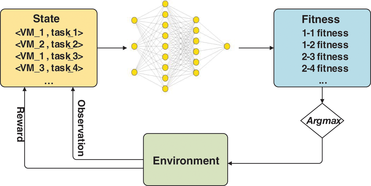
Figure 5: Design of sgent

4.1.5 Training Algorithm

Use a neural network to represent the policy and output a probability distribution for all possible actions. Each episode has a set number of jobs that arrive and are arranged in accordance with the show’s overall concept. When all jobs have completed running, the set comes to an end. The probability space of alternative actions under the current policy is explored and the data obtained is used to enhance the procedure for all tasks, with N sets of N trajectories simulated for each set of jobs in each training iteration.

Specifically, state, action, and reward information is recorded for all time steps of each episode, i.e., {s1, a1, r1,…, sL, aL, rL}, where L is the number of decisions made by the agent. And use these values to calculate the cumulative reward Vt for each time step t of each episode. Algorithm 1 presents the training process of the neural network in Fig. 6. Then, the neural network is trained using the reinforcement algorithm described by the algorithm. A disadvantage of this method is that the gradient estimates can be of high variance. To reduce variance, the mean baseline value is usually subtracted from the returns.

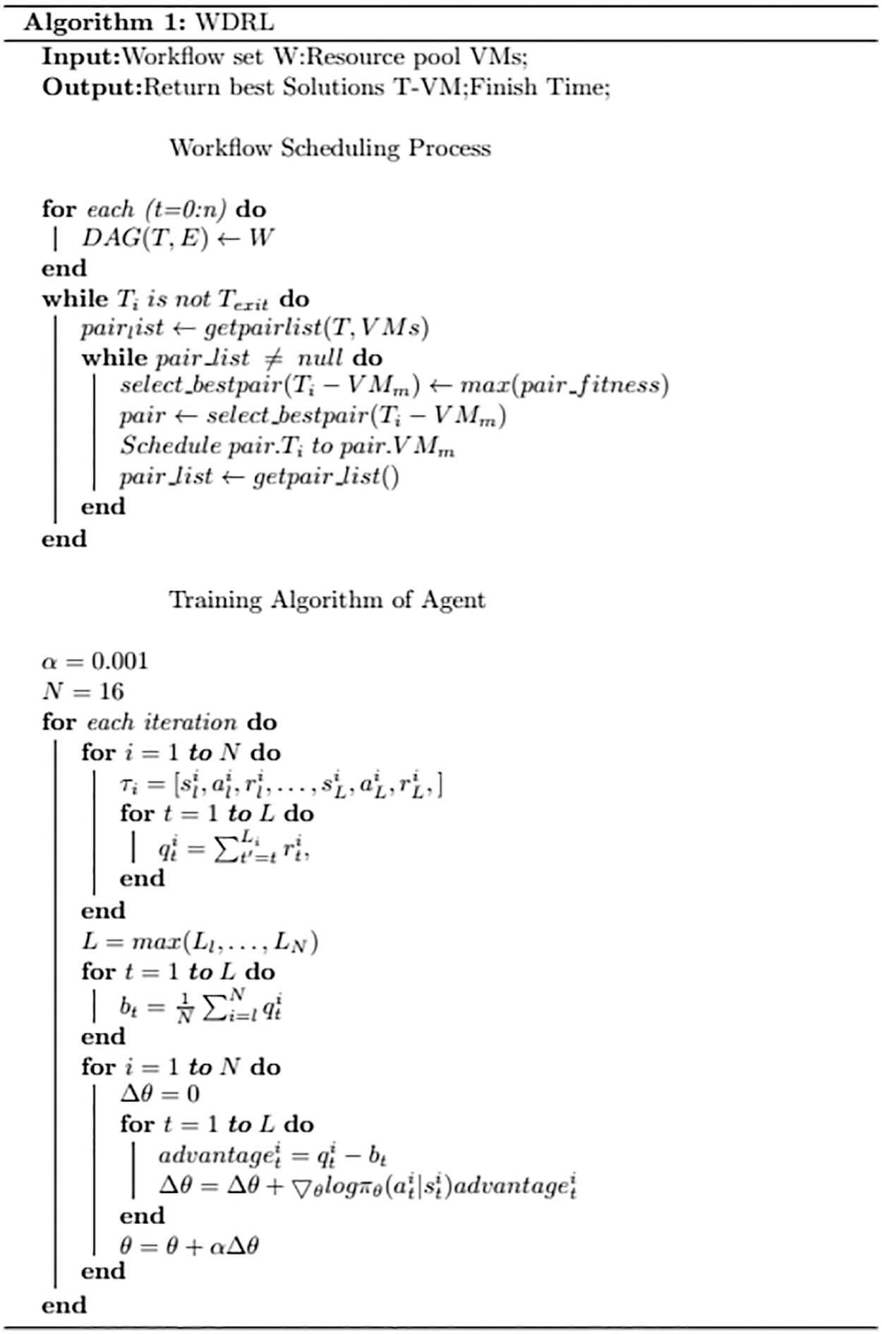
Figure 6: Training algorithm of sgent

5  Experiment and Discussion

To verify the effectiveness of WDRL, a series of case studies are conducted to evaluate the performance of the proposed method and its counterpart in the completion time.

5.1 Experiment Setting

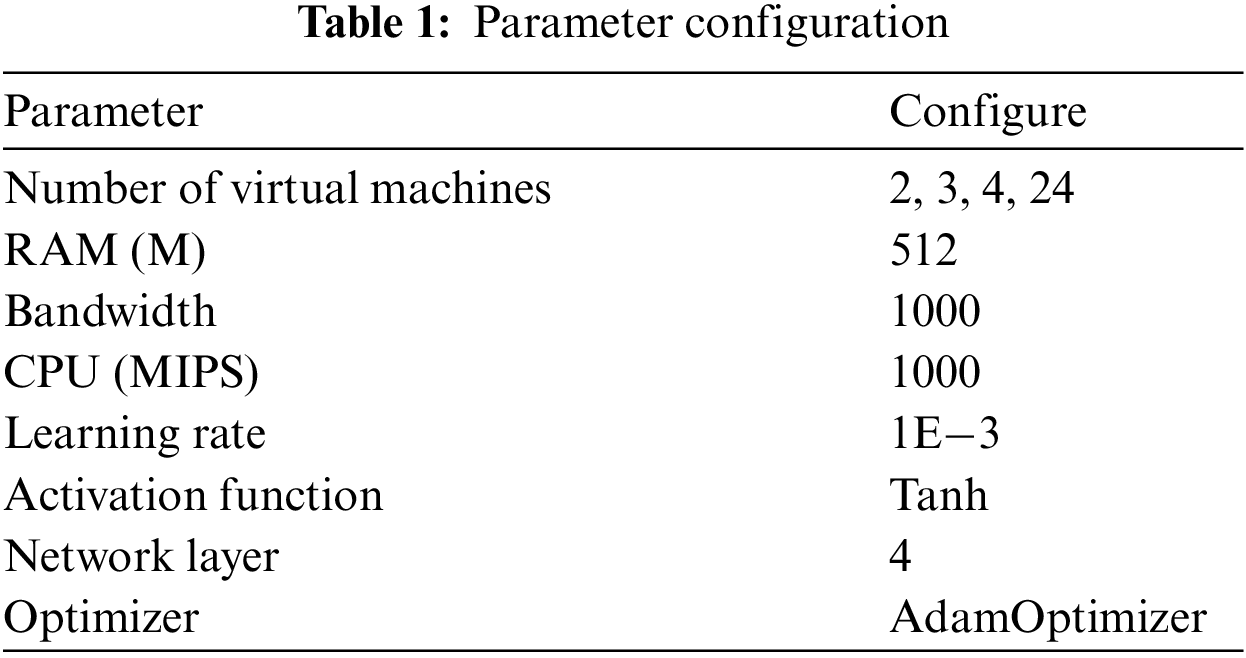
In this section, we will test the fitting ability and scalability of WDRL through a series of simulations. Different factors are used to verify the algorithm’s convergence, including network model, learning rate, and activation function. The specific parameter configuration is shown in Table 1. Finally, the model in the TensorFlow is trained using different magnitudes of a single training set. Simulation experiments are run using the Tensorflow in a Python environment, and the data included Sipht for WorkfowGenerator [21,22] to generate 30, 100, and 1000 data nodes, which are based on models of real applications. These models has parameterized file sizes and task runtime data from execution logs and publications.

The remote sensing data workflow used in the first experiment is a split-window-based water surface temperature inversion process. Water surface temperature inversion [18] is the most widely used algorithm. Its accuracy is about 0.4∼0.8 K. Compared with the single-window algorithm, the split-window algorithm requires fewer parameters and has higher accuracy. It does not require accurate atmospheric profile data, so it is very effective in practical applications. Anding et al. [19] found that the radiance difference between the two infrared bands is proportional to the atmospheric effect that needs to be corrected and proved that in the absence of meteorological data, the radiance values of the two infrared bands could be used to correct the absorption and emission effects of water vapour. Therefore, McClain [20] proposed a multichannel SST algorithm called MCSST (Multi-channel SST). The specific process of batch processing water meter temperature inversion remote sensing product process order is shown in Fig. 7. Pegasus project has released much real-world scientific workflow for academic research. The second experiment verifies the performance applicability of the algorithm using the SIPHT scientific workflow, as shown in Fig. 8.

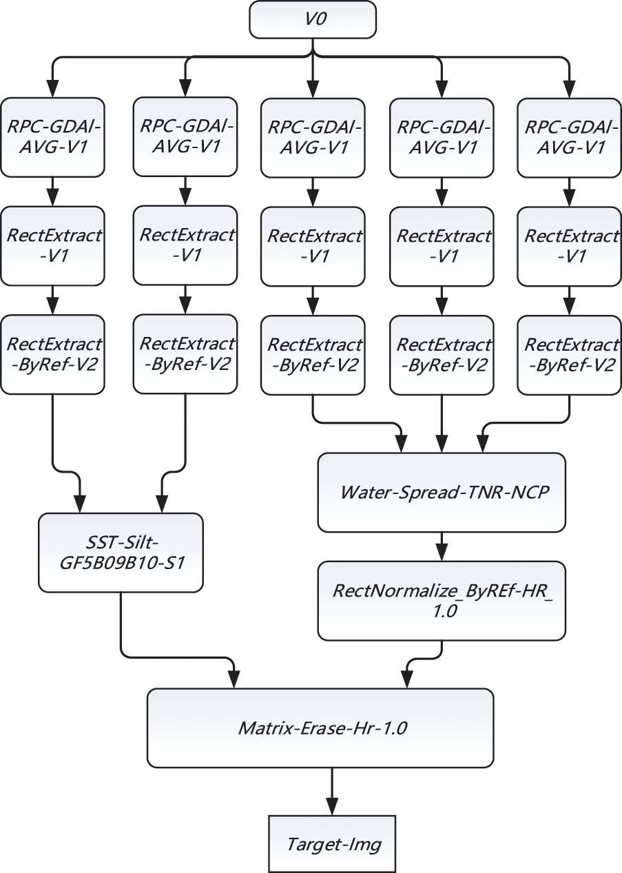
Figure 7: Water meter temperature inversion process

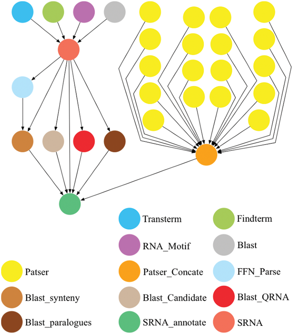
Figure 8: Sipht scientific workflow model

5.2 Experiment Procedure

As shown in Fig. 9, Random algorithm, Heterogeneous Earliest Completion Time (HEFT), Max-min, and Min-min are used as baseline algorithms, respectively. In the remote sensing data processing process with a total number of tasks of 21, the maximum completion time of WDRL is improved by 7.210%, 4.94%, 12.17%, and 9.66% compared with the above 4 algorithms, respectively; WDRL in the test set Sipht with a total number of tasks of 30 is compared with the above 4 algorithm improved by 0.16%, 0.02%, −0.1%, 0.04%; the maximum completion time of WDRL in the test set Sipht with a total number of 100 tasks is improved by 9.548%, 15.919%, 15.53%, 0.77% compared with the above 4 algorithms. In the test set Sipht with a total number of 1000, 24 virtual machines are used due to many tasks, and the maximum completion time of WDRL is improved by 18.49%, 300.8%, 42.1%, and 32.2% compared with the above 4 algorithms. After many subsequent experimental tests, the HEFT algorithm significantly increases the makespan after configuring multiple virtual machines (more than 20 VMs), reflecting its algorithm’s shortcomings.

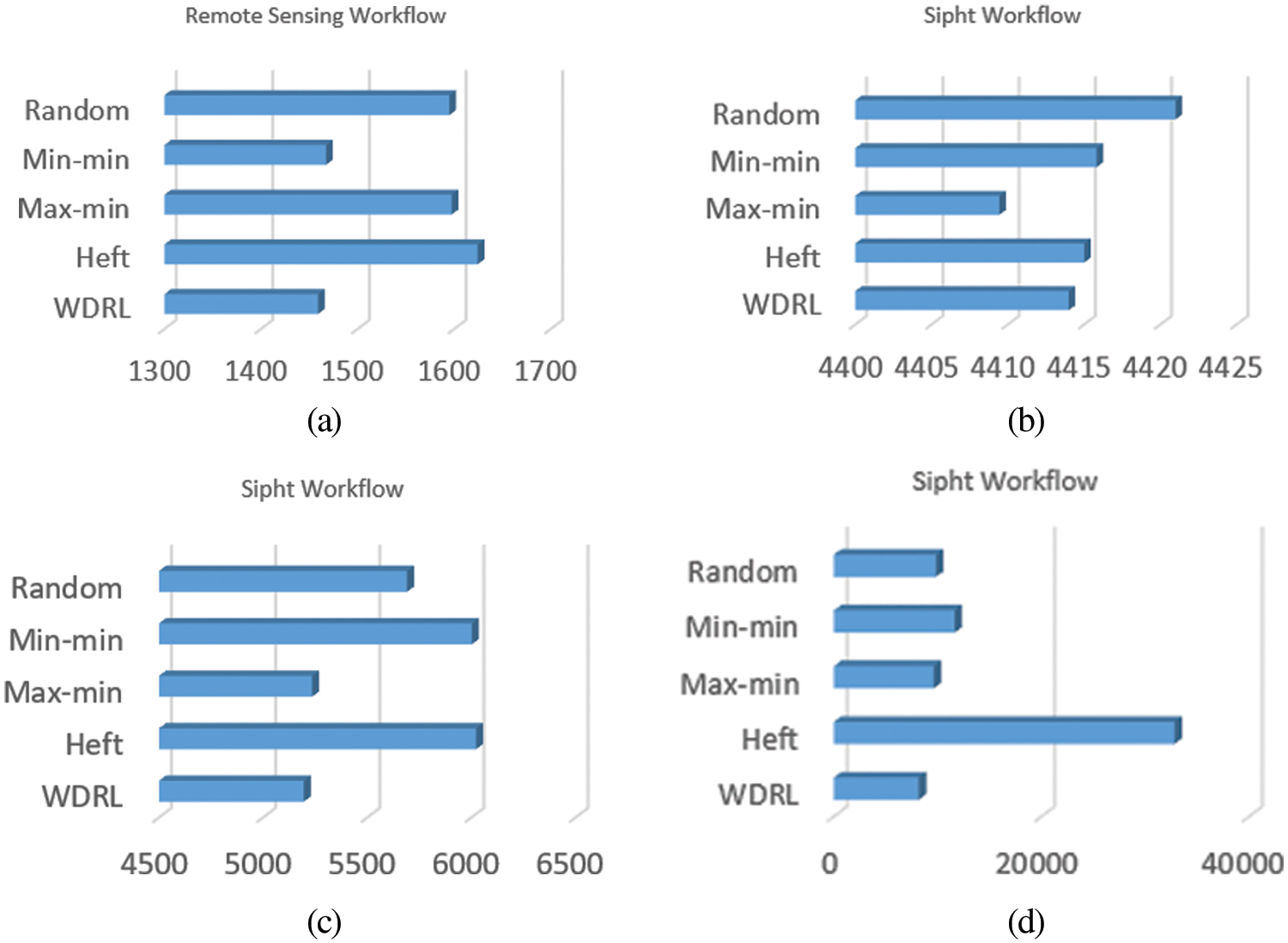
Figure 9: (a) Remote sensing data processing process (Number of tasks is 21) (b) Sipht workflow (Number of tasks is 30) (c) Sipht workflow (Number of tasks is 100) (d) Sipht workflow (Number of tasks is 1000)

5.3 Multi-Machine Stability Tests

As shown in Fig. 10, the algorithm’s performance is tested under different numbers of virtual machines (Num_VM = 2, 3, 4) in the following experiments. The Tensorboard can be used to view the process of the overall decrease in completion times. This stage is where WDRL explores the optimal result. With an increase in training times, the probability of positive reward selection of the algorithm increases, and the action probability with higher profit will be selected during decision-making. During training, 16 trajectories are generated in each iteration of 500 iterations. Therefore, during the experiment, it is possible to see that after 3500 steps, 20 k steps, and 40 k steps in the virtual machine experiments of different magnitudes, the parameter update tends to be stable. The optimization performance of makespan gradually converges to 1727, 1459, and 1281.

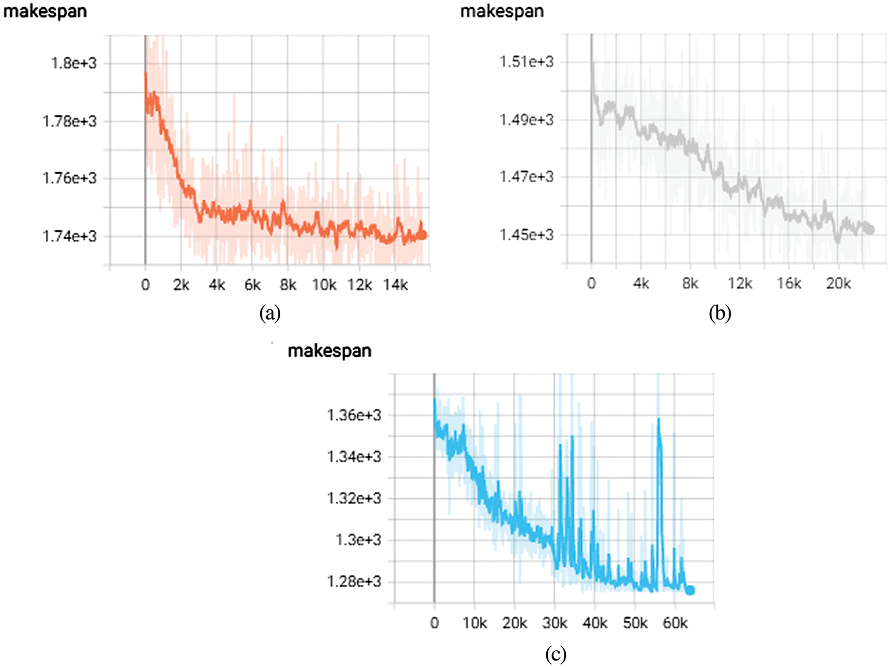
Figure 10: (a) Remote sensing workflow (Num_VM = 2) (b) Remote sensing workflow (Num_VM = 3) (c) Remote sensing workflow (Num_VM = 4)

5.4 Experiment Analysis

As shown in Fig. 11, WDRL has a good optimization effect on the makespan index in four scientific workflows. In the remote sensing data and Sipht workflow, four virtual machines are used for testing. The execution time of Sipht workflow varies significantly in the laboratory with 1000 task nodes, and 24 virtual machines are used for testing. As the number of algorithm training iterations is accumulating, the scheduling solution given by the algorithm gradually stabilizes and outperforms other algorithms. The solution of the algorithm to its scientific workflow is superior to other algorithms, especially when dealing with large-scale task sets. It has outstanding performance advantages, which further proves the convergence and generalization of the WDRL algorithm.

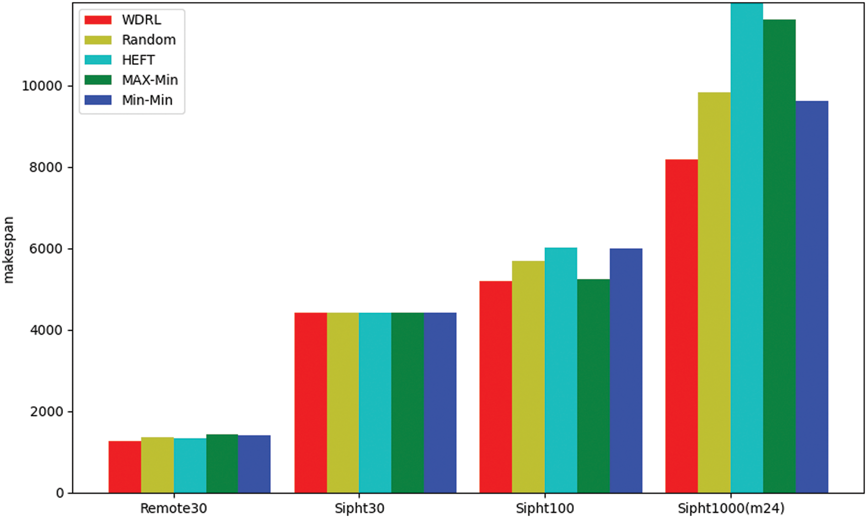
Figure 11: Makespan comparison

6  Related Work

The problem of remote sensing data processing process scheduling is considered one of the main challenges in the cloud environment. The processing of remote sensing data involves a complex multi-stage processing sequence consisting of several independent processing steps, depending on the type of remote sensing application [26,27]. Regional remote sensing data processing has the characteristics of being computationally intensive and data-intensive. Other scholars [28,29] utilized classification and multilayer perceptron regression tree algorithms for land use classification. Wang et al. [30] combined cloud computing and HPC technology to obtain a large-scale remote sensing data processing system suitable for on-demand real-time services and designed a parallel file system for remote sensing data. Ma et al. [31] designed a large-scale remote sensing image stitching method and performed dynamic DAG scheduling on it. Zhang et al. [32] designed a hypergraph (PGH)-based partition group strategy to build a model of shared files and then adopted an optimized task tree (OTT) strategy to deal with the massive remote sensing data processing DAG workflow with data dependencies.

A variety of heuristic algorithms have been proposed for the task scheduling problem [33–35] in the process. However, when tasks depend on each other (for example, a workflow application), the problem becomes apparent. Dependent tasks require a specific order of execution due to their relationship. Many research are based on workflow scheduling that minimizes execution time, such as He et al. [8] using the Min-min algorithm for workflow scheduling. Their proposed method executes small tasks first and then delays large tasks for a long time.

HEFT [7] achieves good performance for the optimization problem of maximum make-time. It is responsible for reducing the search space to a minimum range and achieving higher search efficiency but is very prone to load imbalance. On the other hand, Elzeki et al. [9] used the Max-min algorithm for task scheduling, executing large tasks first, while small tasks had a longer delay time.

7  Conclusion

Resource allocation is crucial for Cloud Computing, especially concerning remote sensing data workflows. Satellite images are equipped with the cloud. The research introduces a workflow scheduling algorithm for remote sensing data processing based on deep reinforcement learning. The algorithm can automatically obtain the fitness calculation method, using the policy gradient method to minimize the makespan directly from experience. Experiments are carried out by tracking trajectory-driven simulations.

The experiments are performed using the Cloudsim platform [36] and two types of real workflows from different scientific fields. WDRL is evaluated with Random algorithm, heterogeneous earliest completion time (HEFT), Max-min, and Min-min. The results demonstrate that WDRL is a promising approach to addressing the issues associated with resource allocation for workflow in the cloud. It outperforms all other algorithms for most carried out tests of remote sensing data processing process and bioinformatics-related Sipht workflows. This is confirmed by the results obtained from the parametric Makespan test. In subsequent Multiple Machines experiments, its convergence is proved.

Future extended research work plans to consider the optimization problem of multiple workflows in the cloud environment and optimize other data centre parameters such as cost and power dissipation.

Author Contributions: The authors confirm contribution to the paper as follows: study conception and design: Y.D. and S.Z.; data collection: S.Z.; analysis and interpretation of results: S.Z. and Y.D.; draft manuscript preparation: S.Z., R.Y.M.L., P.C. and X.G.Y. All authors reviewed the results and approved the final version of the manuscript.

Acknowledgement: The authors wish to thank the Key Research and Promotion Projects of Henan Province. And we would like to thank the Journal of CMES-Computer Modeling in Engineering & Sciences for its support of the research direction of remote sensing data processing in cloud computing.

Funding Statement: This research was funded in part by the Key Research and Promotion Projects of Henan Province under Grant Nos. 212102210079, 222102210052, 222102210007, and 222102210062.

Conflicts of Interest: The authors declare that they have no conflicts of interest to report regarding the present study.

References

1. Zhang, L., Zhang, L., Du, B. (2016). Deep learning for remote sensing data: A technical tutorial on the state of the art. IEEE Geoscience and Remote Sensing Magazine, 4(2), 22–40. DOI 10.1109/MGRS.2016.2540798. [Google Scholar] [CrossRef]
2. Wang, X., Liu, J., Khalaf, O. I., Liu, Z. (2021). Remote sensing monitoring method based on BDS-based maritime joint positioning model. Computer Modeling in Engineering & Sciences, 127(2), 801–818. DOI 10.32604/cmes.2021.013568. [Google Scholar] [CrossRef]
3. Luo, J., Hu, X., Wu, W., Wang, B. (2016). Collaborative computing technology of geographical big data. Journal of Geo-Information Science, 18(5), 590–598. [Google Scholar]
4. Ren, F., Wang, J. (2012). Turning remote sensing to cloud services: Technical research and experiment. Journal of Remote Sensing, 16(6), 1331–1346. [Google Scholar]
5. Adão, T., Hruška, J., Pádua, L., Bessa, J., Peres, E. et al. (2017). Hyperspectral imaging: A review on UAV-based sensors, data processing and applications for agriculture and forestry. Remote Sensing, 9(11), 1110. DOI 10.3390/rs9111110. [Google Scholar] [CrossRef]
6. Xing, L., Li, W., He, M., Tan, X. (2017). Comprehensive multi-objective model to remote sensing data processing task scheduling problem. Concurrency and Computation: Practice and Experience, 29(24), e4248. DOI 10.1002/cpe.4248. [Google Scholar] [CrossRef]
7. Topcuoglu, H., Hariri, S., Wu, M. Y. (2002). Performance-effective and low-complexity task scheduling for heterogeneous computing. IEEE Transactions on Parallel and Distributed Systems, 13(3), 260–274. DOI 10.1109/71.993206. [Google Scholar] [CrossRef]
8. He, X., Sun, X., von Laszewski, G. (2003). QoS guided min-min heuristic for grid task scheduling. Journal of Computer Science and Technology, 18(4), 442–451. DOI 10.1007/BF02948918. [Google Scholar] [CrossRef]
9. Elzeki, O. M., Reshad, M. Z., Elsoud, M. A. (2012). Improved max-min algorithm in cloud computing. International Journal of Computer Applications, 50(12), 1–6. [Google Scholar]
10. Awad, A. I., El-Hefnawy, N. A., Abdel_kader, H. M. (2015). Enhanced particle swarm optimization for task scheduling in cloud computing environments. Procedia Computer Science, 65, 920–929. DOI 10.1016/j.procs.2015.09.064. [Google Scholar] [CrossRef]
11. Akbari, M., Rashidi, H., Alizadeh, S. H. (2017). An enhanced genetic algorithm with new operators for task scheduling in heterogeneous computing systems. Engineering Applications of Artificial Intelligence, 61, 35–46. DOI 10.1016/j.engappai.2017.02.013. [Google Scholar] [CrossRef]
12. Wang, Y., Liu, H., Zheng, W., Xia, Y., Li, Y. et al. (2019). Multi-objective workflow scheduling with deep-Q-network-based multi-agent reinforcement learning. IEEE Access, 7, 39974–39982. DOI 10.1109/Access.6287639. [Google Scholar] [CrossRef]
13. Tong, Z., Chen, H., Deng, X., Li, K., Li, K. (2020). A scheduling scheme in the cloud computing environment using deep Q-learning. Information Sciences, 512, 1170–1191. DOI 10.1016/j.ins.2019.10.035. [Google Scholar] [CrossRef]
14. Zhu, Z., Zhang, G., Li, M., Liu, X. (2015). Evolutionary multi-objective workflow scheduling in cloud. IEEE Transactions on Parallel and Distributed Systems, 27(5), 1344–1357. DOI 10.1109/TPDS.2015.2446459. [Google Scholar] [CrossRef]
15. Watkins, C. J. H., Dayan, P. (1992). Q-learning. Machine Learning, 8, 279–292. DOI 10.1007/BF00992698. [Google Scholar] [CrossRef]
16. Cui, D., Ke, W., Peng, Z., Zuo, J. (2015). Multiple DAGs workflow scheduling algorithm based on reinforcement learning in cloud computing. International Symposium on Computational Intelligence and Intelligent Systems, pp. 305–311. Springer, Singapore. [Google Scholar]
17. Sutton, R. S., McAllester, D., Singh, S., Mansour, Y. (1999). Policy gradient methods for reinforcement learning with function approximation. Advances in Neural Information Processing Systems, 12, 1–7. [Google Scholar]
18. Gao, Y. C., Liang, H. Y., Li, J. G., Gu, X. F. (2011). Method of water surface temperature retrieval based on HJ-1B. Remote Sensing Information, 2, 9–13. [Google Scholar]
19. Walton, C. C. (1988). Nonlinear multichannel algorithms for estimating sea surface temperature with AVHRR satellite data. Journal of Applied Meteorology and Climatology, 27(2), 115–124. DOI 10.1175/1520-0450(1988)027<0115:NMAFES>2.0.CO;2. [Google Scholar] [CrossRef]
20. Hulley, G. C., Hook, S. J., Schneider, P. (2011). Optimized split-window coefficients for deriving surface temperatures from inland water bodies. Remote Sensing of Environment, 115(12), 3758–3769. DOI 10.1016/j.rse.2011.09.014. [Google Scholar] [CrossRef]
21. Bharathi, S., Chervenak, A., Deelman, E., Mehta, G., Su, M. H. et al. (2008). Characterization of scientific workflows. 2008 Third Workshop on Workflows in Support of Large-Scale Science, pp. 1–10. Austin, TX, USA. DOI 10.1109/WORKS.2008.4723958. [Google Scholar] [CrossRef]
22. Ludäscher, B., Altintas, I., Berkley, C., Higgins, D., Jaeger, E. et al. (2006). Scientific workflow management and the Kepler system. Concurrency and Computation: Practice and Experience, 18(10), 1039–1065. DOI 10.1002/(ISSN)1532-0634. [Google Scholar] [CrossRef]
23. Juve, G., Chervenak, A., Deelman, E., Bharathi, S., Mehta, G. et al. (2013). Characterizing and profiling scientific workflows. Future Generation Computer Systems, 29(3), 682–692. DOI 10.1016/j.future.2012.08.015. [Google Scholar] [CrossRef]
24. Hagan, M. T., Demuth, H. B., Beale, M. (1997). Neural network design. USA: PWS Publishing Co. [Google Scholar]
25. Hastings, W. K. (1970. Monte Carlo sampling methods using markov chains and their applications, Biometrika, 57(1), 97–109. DOI 10.1093/biomet/57.1.97. [Google Scholar] [CrossRef]
26. Li, C., Yue, X. G., (2018). Ultrasonic excitation-fiber bragg grating sensing technique for damage identification. International Journal of Online Engineering, 14(7), 124–136. DOI: 10.3991/ijoe.v14i07.8969. [Google Scholar] [CrossRef]
27. Zhang, J., Lu, C., Wang, J., Yue, X. G., Lim, S. J. et al. (2020). Training convolutional neural networks with multi-size images and triplet loss for remote sensing scene classification. Sensors, 20(4), 1188. DOI 10.3390/s20041188. [Google Scholar] [CrossRef]
28. Zeng, F. F., Feng, J., Zhang, Y., Tsou, J. Y., Xue, T. et al. (2021). Comparative study of factors contributing to land surface temperature in high-density built environments in megacities using satellite imagery. Sustainability, 13(24),13706. DOI 10.3390/su132413706. [Google Scholar] [CrossRef]
29. Li, R. Y. M., Chau, K. W., Li, H. C. Y., Zeng, F., Tang, B. et al. (2021). Remote sensing, heat island effect and housing price prediction via AutoML. In: Ahram, T. (Ed.Advances in intelligent systems and computing, vol. 1213. Cham: Springer. [Google Scholar]
30. Wang, L., Ma, Y., Yan, J., Chang, V., Zomaya, A. Y. (2018). pipsCloud: High performance cloud computing for remote sensing big data management and processing. Future Generation Computer Systems, 78, 353–368. DOI 10.1016/j.future.2016.06.009. [Google Scholar] [CrossRef]
31. Ma, Y., Wang, L., Zomaya, A. Y., Chen, D., Ranjan, R. (2013). Task-tree based large-scale mosaicking for massive remote sensed imageries with dynamic dag scheduling. IEEE Transactions on Parallel and Distributed Systems, 25(8), 2126–2137. DOI 10.1109/TPDS.2013.272. [Google Scholar] [CrossRef]
32. Zhang, W., Wang, L., Ma, Y., Liu, D. (2014). Design and implementation of task scheduling strategies for massive remote sensing data processing across multiple data centers. Software: Practice and Experience, 44(7), 873–886. [Google Scholar]
33. Li, F., Hu, B. (2019). Deepjs: Job scheduling based on deep reinforcement learning in cloud data center. Proceedings of the 2019 4th International Conference on big Data and Computing (ICBDC 2019), pp. 48–53. New York, NY, USA, Association for Computing Machinery. DOI 10.1145/3335484.3335513. [Google Scholar] [CrossRef]
34. Liu, Z., Zhang, S., Liu, Y., Wang, X., Yin, D. (2021). Run-time dynamic resource adjustment for mitigating skew in MapReduce. Computer Modeling in Engineering & Sciences, 126(2), 771–790. DOI 10.32604/cmes.2021.013244. [Google Scholar] [CrossRef]
35. Lu, W., Guo, S., Song, T., Li, Y. (2022). Analysis of multi-AGVs management system and key issues: A review. Computer Modeling in Engineering & Sciences, 131(3), 1197–1227. DOI 10.32604/cmes.2022.019770. [Google Scholar] [CrossRef]
36. Calheiros, R. N., Ranjan, R., Beloglazov, A., de Rose, C. A., Buyya, R. (2011). CloudSim: A toolkit for modeling and simulation of cloud computing environments and evaluation of resource provisioning algorithms. Software: Practice and Experience, 41(1), 23–50. [Google Scholar]
Cite This Article
Copyright © 2023 The Author(s). Published by Tech Science Press.
This work is licensed under a Creative Commons Attribution 4.0 International License , which permits unrestricted use, distribution, and reproduction in any medium, provided the original work is properly cited.
Downloads
Citation Tools