
 Submit a Paper
 Propose a Special lssue
 Open Access
ARTICLE

Novel Hybrid XGBoost Model to Forecast Soil Shear Strength Based on Some Soil Index Tests
1
Department of Civil Engineering, Faculty of Engineering, Lorestan University, Khorramabad, 6815144316, Iran
2
Department of Civil Engineering, Faculty of Engineering, Universiti Malaya, Kuala Lumpur, 50603, Malaysia
3
Department of Geology, Faculty of Sciences, Lorestan University, Khorramabad, 6815144316, Iran
4
Department of Urban Planning, Engineering Networks and Systems, Institute of Architecture and Construction,
South Ural State University, Chelyabinsk, 454080, Russia
* Corresponding Author: Yasin Abdi. Email:
(This article belongs to the Special Issue: Computational Intelligent Systems for Solving Complex Engineering Problems: Principles and Applications)
Computer Modeling in Engineering & Sciences 2023, 136(3), 2527-2550. https://doi.org/10.32604/cmes.2023.026531
Received 10 September 2022; Accepted 11 November 2022; Issue published 09 March 2023
 View Full Text
 Download PDF
Abstract
When building geotechnical constructions like retaining walls and dams is of interest, one of the most important factors to consider is the soil’s shear strength parameters. This study makes an effort to propose a novel predictive model of shear strength. The study implements an extreme gradient boosting (XGBoost) technique coupled with a powerful optimization algorithm, the salp swarm algorithm (SSA), to predict the shear strength of various soils. To do this, a database consisting of 152 sets of data is prepared where the shear strength (τ) of the soil is considered as the model output and some soil index tests (e.g., dry unit weight, water content, and plasticity index) are set as model inputs. The model is designed and tuned using both effective parameters of XGBoost and SSA, and the most accurate model is introduced in this study. The prediction performance of the SSA-XGBoost model is assessed based on the coefficient of determination (R2) and variance account for (VAF). Overall, the obtained values of R2 and VAF (0.977 and 0.849) and (97.714% and 84.936%) for training and testing sets, respectively, confirm the workability of the developed model in forecasting the soil shear strength. To investigate the model generalization, the prediction performance of the model is tested for another 30 sets of data (validation data). The validation results (e.g., R2 of 0.805) suggest the workability of the proposed model. Overall, findings suggest that when the shear strength of the soil cannot be determined directly, the proposed hybrid XGBoost-SSA model can be utilized to assess this parameter.Keywords
Nomenclature
| ANN | Artificial Neural Network |
| GEP | Genetic Expression Programming |
| SVM | Support Vector Machine |
| ANFIS | Adaptive Neuro-Fuzzy Inference System |
| HGSO | Henry Gas Solubility Optimization |
| GA | Genetic Algorithm |
| PSO | Particle Swarm Optimization |
| SSA | Salp Swarm Algorithm |
| VAF | Variance Account For |
| τ | Shear Strength |
| Internal Friction Angle | |
| c | Cohesion |
| γd | Dry Unit Weight |
| PPS4 | Percent Passing Sieves No 4 |
| PPS40 | Percent Passing Sieves No 40 |
| Wn | Water Content |
| PL | Plastic Limit |
| LL | Liquid Limit |
It is well established that soil failure generally occurs in the form of shearing. Hence, proper determination of soil shear strength is crucial in designing geotechnical structures such as retaining walls, and foundations. Although there is a direct method and standard procedure for determining the soil shear strength, the feasibility of indirect methods in estimating the shear strength of soil is also underlined in literature, which is mainly due to the fact that indirect methods are quick tools and economic. Indirect methods include conventional empirical correlations between soil index tests and shear strength parameters like cohesion and internal friction angle of the soil. For example, Hatanaka et al. [1] reported an empirical correlation between penetration resistance and friction angle of cohesionless soils. Nevertheless, in recent past years, the implementation of artificial intelligence and reliability analysis-based methods in solving civil and geotechnical engineering problems has received considerable attention [2–25]. It is worth mentioning that the implementation of soft computing techniques is of interest when the contact nature between parameters is nonlinear.
On the other hand, the shear strength of the soil is a function of various parameters and the relationship between these influential parameters and shear strength is complex and nonlinear. Hence, the implementation of artificial intelligence techniques, is beneficial as suggested by many researchers. For example, Khanlari et al. [26] investigated the feasibility of an artificial neural network (ANN) in assessing the shear strength parameters of soil (i.e., cohesion and internal friction angle). Their suggested predictive model comprised several input parameters including plasticity index (PI), soil density, and the passing percentage of different sieves (i.e., No. 200, No. 40, and No. 4). They used 200 sets of data for their model development. Their findings suggest (correlation coefficient of 0.91) that their proposed model can be implemented for estimating the shear strength parameters. Kayadelen et al. [27] showed the workability of genetic expression programming (GEP) in estimating the effective angle of shearing resistance of soils. Khan et al. [28] developed a new model called the Functional Network (FN) to forecast the residual strength of the soil.
Das et al. [29] utilized ANN to assess the residual strength of clays. In another study, Das et al. [30] used support vector machine (SVM) and ANN techniques to estimate the residual strength of the soil. Ding et al. [31] developed an intelligent predictive model of soil shear strength. Their model inputs comprise plastic and liquid limits, clay content, moisture content, void ratio as well as specific gravity. Their recommended model was based on an adaptive neuro-fuzzy inference system (ANFIS) improved with henry gas solubility optimization (HGSO). According to their results, the coefficient of determination value of 0.954 shows the feasibility of the aforementioned hybrid model in estimating the shear strength of the soil. It should be mentioned that they used 127 sets of data for constructing their models. In another study, Armaghani et al. [32] suggested that the neuro-imperialism method can be implemented for the indirect estimation of shear strength parameters of sandy soils. According to their study, the inputs of their proposed model were fiber length and percentage, deviatoric stress as well as pore water pressure values. Their findings show that the predictive models which were made with improved ANNs outperform conventional ANN models. It is worth mentioning that the utilized sand in their study was reinforced with fibers and they tested the performance of the models using 30 sets of data. Kanungo et al. [33] implemented a regression tree and ANNs for assessing the unsaturated soil shear strength parameters. Kiran et al. [34] proposed an ANN-based predictive model of soil shear strength. Their model inputs were soil index properties including Atterberg limits, dry and bulk densities as well as the percentages of gravel, sand, and clay, respectively. They used 300 sets of data for establishing their proposed ANN-based predictive model.
In another study, Tizpa et al. [35] recommended an ANN-based predictive model of effective friction angle of shearing. Overall, they compiled 105 sets of data. The inputs of their proposed model were coarse content, fine content, liquid limit, soil bulk density, and shearing rate. According to their sensitivity analysis, among the aforementioned input parameters, soil density was the most influential parameter. Pham et al. [36] utilized machine learning techniques for assessing the shear strength of soft soils. Using 188 clay soil samples, they compared the prediction performance of different soft computing techniques including ANN, support vector regression (SVR), ANFIS improved with Genetic algorithm (GA), and Particle Swarm Optimization (PSO) algorithm. Their findings showed that the PSO-ANFIS-based predictive model of shear strength with an R-value of 0.60 is a relatively good predictor. The input parameters of their recommended model were clay content, liquid limit, plastic limit, moisture content, consistency index, and plastic index. In another study, Kaya [37] compiled a dataset from another study (i.e., Stark et al. [38]) and showed that effective normal stress, activity, clay fraction, liquid and plastic limits can form the inputs of the ANN-based predictive model of residual friction angle of soil. The coefficient of determination value of 0.93 suggests the reliability of their developed model.
Tien Bui et al. [39] implemented a least square support vector machine and cuckoo search optimization algorithm for assessing the shear strength of soils. They used 332 sets of data for model construction. The inputs of their model comprise moisture content, specific gravity, soil density, liquid and plastic limits, liquid index, sample depth, sand, loam, and clay percentages, respectively. The R2 value of 0.885 suggests the workability of their proposed predictive model for predicting shear strength. Hashemi Jokar et al. [40] proposed the use of ANFIS for predicting unsaturated soil shear strength. According to their study, the conventional parameters in the empirical models can be used as inputs for the intelligent-based predictive models. Therefore, the inputs of their ANFIS-based predictive model include net normal stress, angle of frictional resistance, matric suction, and effective cohesion. They used 95 sets of data for model development. Overall, their findings suggest that the ANFIS is a capable tool for estimating the shear strength of unsaturated soils.
Ly et al. [41] mentioned that SVR is a useful tool in predicting the shear strength of the soil. They used 500 sets of data for model construction. The input of their models consisted of void ratio, specific gravity, clay and moisture contents as well as liquid and plastic limits. The R2 value of 0.91 recommends the feasibility of their proposed SVR-based predictive model. Mousavi et al. [42] proposed an ANN-based predictive model of friction angle using 27 sets of data. The input layer of their proposed model comprises grain size distribution parameters as well as the relative density of the soil. Chao et al. [43] conducted a comparative study using soft computing techniques for estimating soil shear strength. Using 316 sets of data, they assessed the shear strength between the soil and the Geocomposite drainage layer. The input parameters for their developed models were normal stress, soil density, moisture saturation of the soil, thickness and type of drainage core, soil type, shearing surface, consolidation condition, and geotextile specifications. Jain et al. [44] utilized 198 sets of experimental data for developing an ANN-based predictive model of shear strength parameters. Compaction energy, degree of saturation, and dry density formed the input layer of their proposed ANN-based predictive model. A regression coefficient equal to 0.94 recommends the feasibility of their proposed models. Zhang et al. [45] utilized extreme gradient boosting to estimate the shear strength of soft soils. They used five input parameters, including vertical effective stress, plastic and liquid limits, preconsolidation stress, and natural water content.
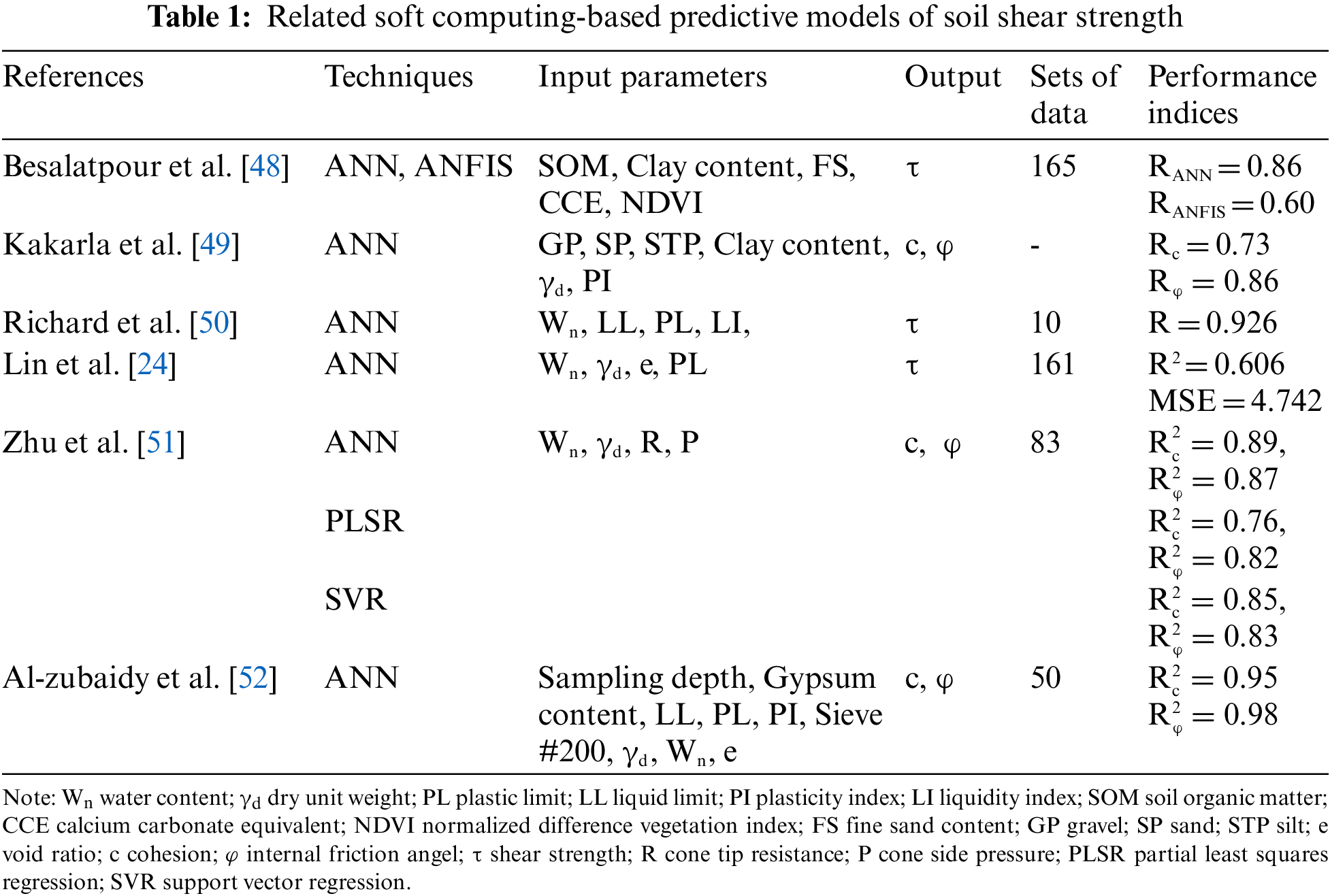
Dutta et al. [46] proposed a soft computing-based predictive model of friction angle. They compiled 60 sets of data for model construction. The input layer of their proposed model comprises sand content, clay content, plastic limit, and liquid limit. The R2 value of 0.96 for their testing data suggests the workability of their proposed ANN-based predictor. Mohammadi et al. [47] estimated soil shear strength parameters using ANN and multivariate regression. They used 108 sets of data for their modeling. The input parameters of their proposed models include percentages of gravel, sand, silt, and clay, respectively, Atterberg limits, and density. The R2 values of 0.885 and 0.845 for the ANN-based predictive model of cohesion and ANN-based predictive model of friction angle recommend the feasibility of neural networks in assessing the engineering properties of soils. A number of works done on the prediction of shear strength using soft computing techniques are presented in Table 1.
This study aimed to propose a novel intelligent predictive model of soil shear strength, i.e., extreme gradient boosting-salp swarm algorithm (XGBoost-SSA). The proposed model is based on the 152 experiments performed by authors. The point that in this study XGBoost technique is coupled with the salp swarm algorithm for assessing the soil shear strength differentiates the presented work from other related studies. From the authors’ perspective, publishing the results of new laboratory tests for this problem and verifying the previously proposed techniques with various datasets for the same type of prediction problems are advantageous. Additionally, repetition of this type of study can establish common sense and provide broad observation chance about the relation between the problem of interest and predictive methods. Nevertheless, in this study, after the introduction and reviewing the related works in Section 1, the materials, experimental methods, and the implemented database are discussed in Section 2. Section 3 deals with the soft computing-based methodology and the relevant modeling procedure, respectively. In Section 4, results and discussion are presented and in Section 5 conclusion remarks are discussed.
2 Materials, Experimental Methods, and Implemented Database
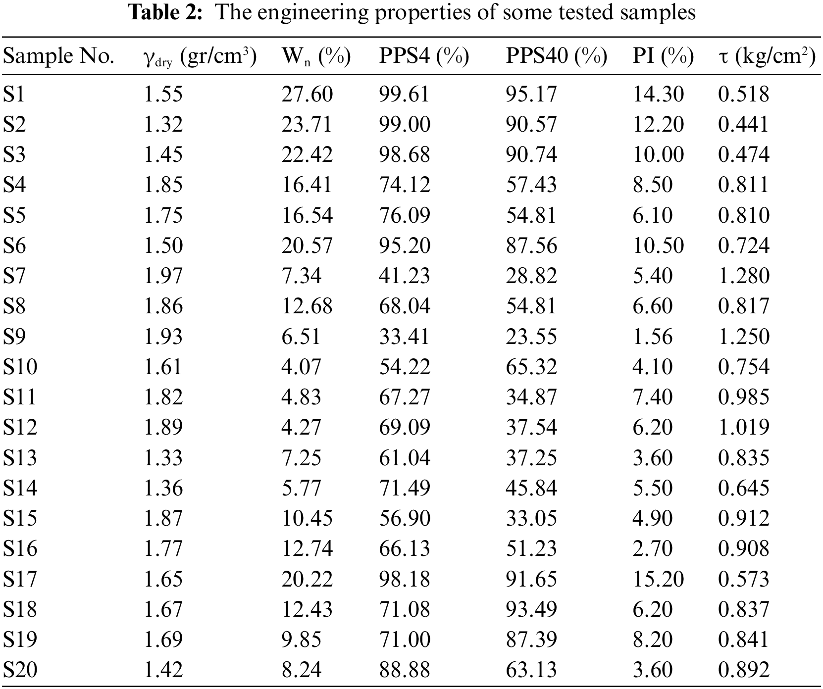
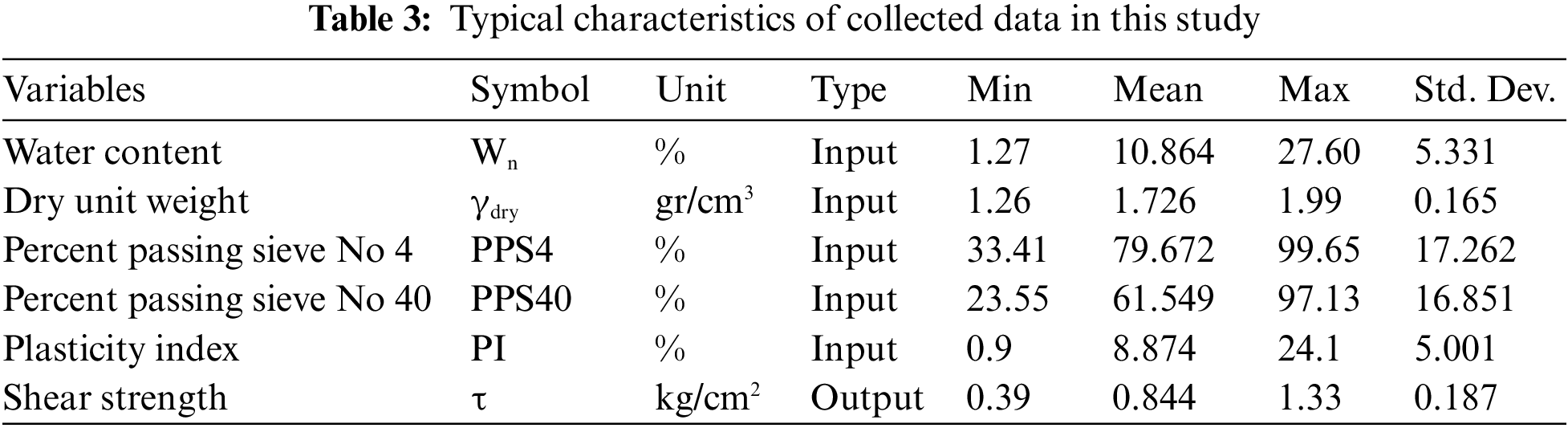
In this study, shear strength values were assessed using a database consisting of 152 datasets. For this purpose, different soil specimens were gathered from both subsurface and surface resources in Zanjan Province in the West of Iran (Fig. 1). Next, the soil samples were characterized in terms of engineering properties such as dry unit weight (γd), percent passing sieve No 4 (PPS4), percent passing sieve No 40 (PPS40), shear strength (τ), water content (Wn), and plasticity index (PI). Table 2 indicates the engineering properties of some samples which were utilized in this work. A summary of the statistical values of the inputs and output is also presented in Table 3. All tests were carried out in accordance with ASTM D3080 [53] in the laboratory of Hamedan Sinab-Gharb Consulting Engineers. In this study, the shear strength is set as the output variable. Furthermore, the input variables comprise γd, PPS4, PPS40, Wn, and PI.
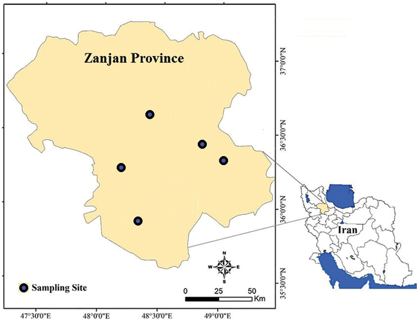
Figure 1: The location of the sampling sites in Zanjan Province
Shear strength of a soil mass, as the output variable of this study, is the internal resistance of each unit area of the soil against sliding and failure along any plane inside it [54]. This parameter is of prime importance in bearing capacity and slope stability analyses. The soil failure is attributed to a critical combination of normal and shearing stress. Therefore, the relationship between these two types of stress on a failure surface of a soil mass is expressed by Eq. (1):
where σn denotes the normal stress on the failure plane (kg/cm2), c shows cohesion (kg/cm2), and
Soil shear strength parameters (i.e., c and
Water content (Wn) is the ratio of the water weight to the solids’ weight in a specific volume of soil. This parameter influences the soil’s shear strength by lowering the cohesive forces between soil solids. Water content also causes the soil’s saturation. The shear strength of soils declines with increasing the water content [56]. Hence, we considered this parameter in estimating the shear strength of the studied soil samples. In the laboratory, Wn is determined by oven drying the soil specimen. On the other hand, field testing of Wn is carried out using the alcohol-burning method. This parameter is calculated using Eq. (2) as follows [54,55]:
where Ws and Ww are the weights of soil sample solids and soil’s water, respectively. The Wn of a soil sample is determined by weighing soil sample and placing it in an oven at 110°C ± 5°C until the weight of the sample reaches a constant state. In this condition, all water content of the soil is released. For most soils, a constant weight is achieved at about 24 h. The soil sample is removed from the oven, cooled, and weighed. As shown in Table 3, the Wn values of the studied soil range from 1.27% to 27.60%.
The plasticity index (PI) is the range of water content over which the soil deforms in a plastic form. Soil’s PI is positively correlated with its shear strength. Mathematically, PI is expressed as the difference between the plastic limit (PL) and liquid limit (LL), as follows:
where LL and PL are determined using the Atterberg tools [54]. In this study, the PI values vary from 0.90% to 24.10% (Table 3).
Dry unit weight (γd) is the weight of a dry soil per unit volume. Dry unit weight can be calculated using the following equation:
where Ws is considered as the weight of solids of the soil sample, and V is the total volume of the soil sample. The increase in dry unit weight can enhance the shear strength of soil. As shown in Table 3, the dry unit weight values of soil samples vary from 1.26 to 1.99 gr/cm3.
2.5 The Particle Size Distribution Analysis
The sieve analysis was performed to determine grain size distribution. In this research, percent passing sieves No 4 (PPS4), and percent passing sieves No 40 (PPS40) were used to predict soils’ shear strength using the hybrid SSA-XGBoost technique. As shown in Table 3, the values of PPS4 and PPS40 are 33.41–99.65 and 23.55–97.13, respectively.
To estimate the linear relationship among variables used in this study, a correlation matrix was produced. Based on this, the correlation matrix was created by applying the bivariate correlation method. In this analysis, Pearson’s correlation coefficients between τ, being the dependent variable, and the other utilized soil parameters, being independent variables, were investigated. In Table 4, Pearson’s correlation coefficients (R values) are presented.
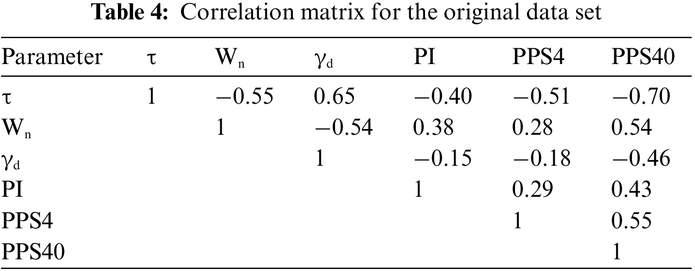
To expound on the correlations between these variables, the scatter plot matrix was also employed. It contains all the pair-wise scatter plots of the variables on a single page in a matrix format, as depicted in Fig. 2. The results show that only the input variable, γdry, positively correlates with the shear strength. For the input variables such as Wn, PPS4, PPS40, and PI, negative correlations with the shear strength were observed. Overall, the five input variables do not show a strong correlation with shear strength. Pearson’s R value of 0.699 between PPS40 and shear strength suggests the aforementioned conclusion. Additionally, as expected the mutual correlations between input variables (i.e., Wn, γdry, PPS4, PPS40, and PI) were weak. Note that in this section, only a simple linear relationship between these five variables and shear strength is discussed.
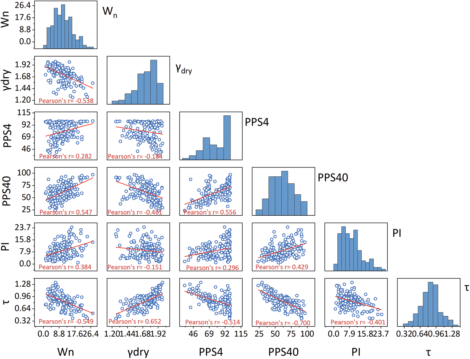
Figure 2: Scatters plot matrix of the data samples
3 Soft Computing-Based Methodology
Extreme gradient boosting (XGBoost), a multi-threaded implementation of the gradient boosting decision tree (GBDT), is a highly efficient machine learning algorithm that evolved from the traditional machine learning classification and regression tree (CART) [57]. Fig. 3 shows that XGBoost is an ensemble tree-based model and it has a highly scalable end-to-end tree boosting system. The basic idea of XGBoost is the stacking strategy as well as parallel and distributed computing [58,59]. XGBoost concatenates multiple CARTs and then inputs the original training set into the first regression tree to generate a weak learning model; after that, XGBoost collects the training errors generated by the first weak learning model to build a new data set with the error. Next, the new data set is considered as new training data which is utilized for training the second regression tree. The above steps continuously repeat and the loop ends until the value of the objective function is less than the desired threshold. Ultimately, the predicted results can be obtained by summing the results of multiple trees.
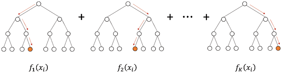
Figure 3: Structure of the XGBoost model
The mathematical model of XGBoost is as follows:
For the dataset D with n samples and m features
where
In Eq. (5), the prediction results for sample i after the t-th iteration is:
Based on Eq. (9), the objective function can be transformed into the following form:
Then, the Taylor expansion of the objective function is performed and the first three terms are taken (removing the higher-order infinitesimal terms). The new objective function takes the following form:
where
For an XGBoost model, determining the optimal hyperparameters is a crucial task because it can significantly affect the performance of the constructed XGBoost model. The dominant hyperparameters of the XGBoost model in the present research are elaborated as follows:
The number of estimators: The maximum number of gradient boosted trees. In general, if this value is too low, the model will underfit, and if the value is too high, the computation cost will be considerably increased.
Learning rate: Step size shrinkage is used in each iteration. To avoid overfitting, step size shrinking was implemented in the update because it can shrink the feature weights to make the boosting process more conservative.
Subsample: Subsample ratio of the training instances when growing trees. This hyperparameter can help the XGBoost model to prevent overfitting.
The salp swarm algorithm (SSA) is a swarm intelligence optimization algorithm that mimics the locomotion and foraging behavior of the salp swarm [60]. In deep oceans, a swarm formed by salps is called a salp chain. This “chain” shape keeps the salp moving in a certain order. According to the position of individual salp, the salps are divided into the leader and followers. As the name implies, the leader has the best judgment of the surrounding environmental situation and ranks at the head of the chain. However, unlike other swarms’ behavior, the leader in SSA no longer directly dominates the movement direction of the entire salps, but only directly guides the position update of the salps immediately next to it. In this case, the leader’s guidance to the subsequent salps decreases sharply step by step, which helps the subsequent salps to retain their diversity rather than only moving towards the leaders. The mathematical model of the SSA is as follows.
3.2.1 Initialize the Population
The search domain space is assumed to be an
where
3.2.2 Update of the Leader’s Position
The first leader (salp) is responsible for searching for food (in the search domain) and guiding the movement of the subsequent salps. The following equation is used to update the position of the leader:
where
where l and
3.2.3 Update the Followers’ Positions
In the SSA, the followers in a chain follow the leader sequentially. The positions of followers are related to their initial positions, movement speed, and acceleration. Moreover, their motion follows Newton’s law [60,61]. The movement distance of the followers can be determined as follows:
where R denotes the movement distance of the followers, a denotes the acceleration and its calculation formula is
Then, the updated positions of the followers can be expressed as follows:
where
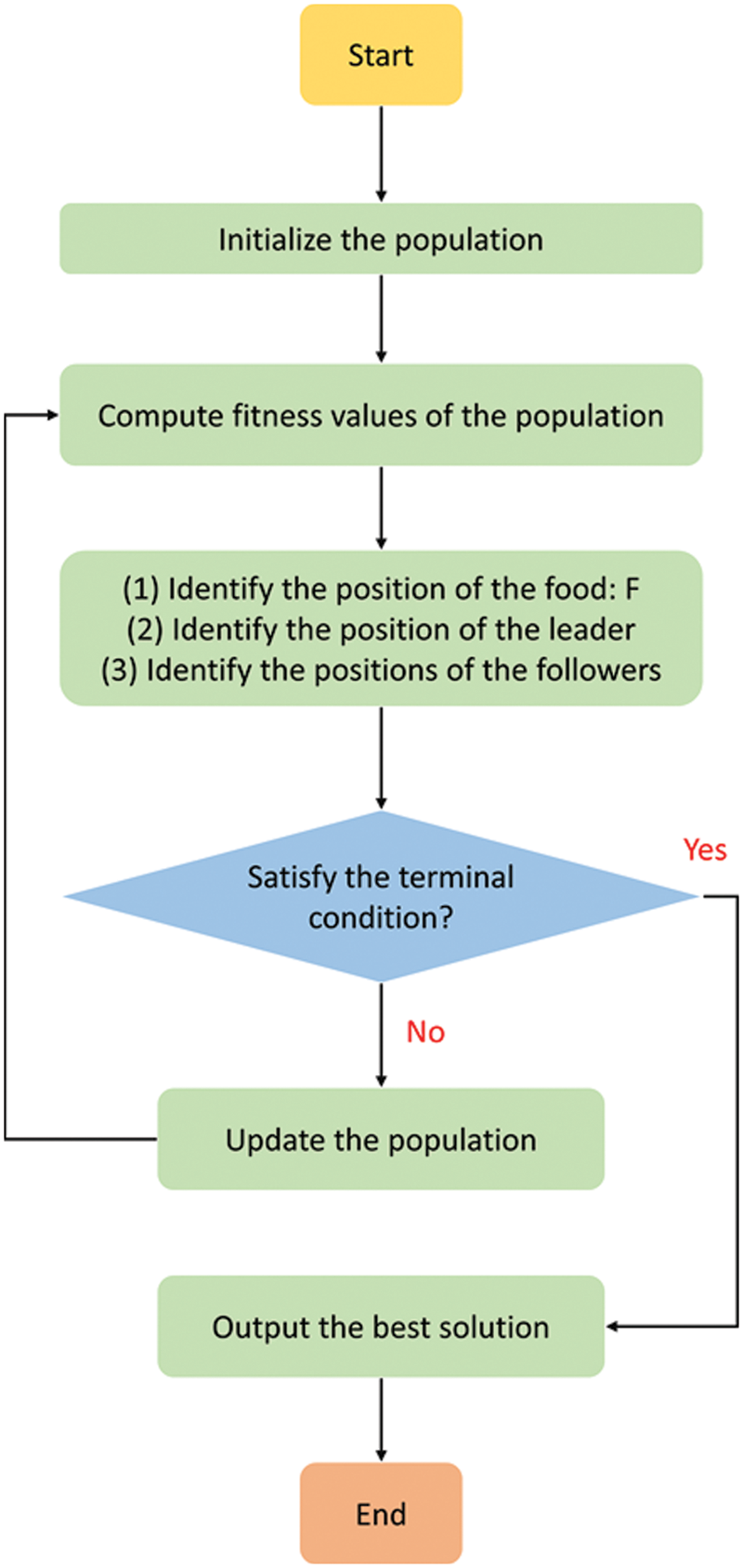
Figure 4: Flowchart of the salp swarm algorithm (SSA)
3.3 Optimized XGBoost-Based Models
Owing to the parameters involved in the XGBoost model with highly unknown space domains, tuning its hyperparameter is more complicated compared to other tree-based models such as the random forests model. Generally, the results of manual tuning are unsatisfactory. Therefore, in this section, the metaheuristic optimization algorithm SSA is used to capture the best hyperparameters of the XGBoost model. Before constructing the hybrid model, the dataset including 152 samples is randomly split into two parts, i.e., 80% for the training set (121 samples) and 20% for the testing set (31 samples). Then, the SSA is utilized to optimize the XGBoost model. The main steps for constructing the hybrid SSA-XGBoost model are shown as follows:
Step 1: Determine the objective function that needs to be optimized by SSA. First, the primary XGBoost model is established and the hyperparameters, i.e., learning rate and subsample, are set as the optimization objectives in the XGBoost model. It should be mentioned that the SSA algorithm is generally used to solve minimization problems. Hence, the objective function is defined as the function of the root mean squared error (RMSE), which presents the difference between the target values and the values predicted by the XGBoost model. In this way, the SSA will optimize the XGBoost model to seek the minimum RMSE value (the optimal values of the hyperparameters). During the process, a 5-fold cross-validation method was used to reduce the likelihood of accidental results.
Step 2: Determine the range of the hyperparameters. In the present study, the range of learning rate was set to [0.01, 0.50], the range of subsample was set to [0.2, 0.8], and the number of estimators was set to 50.
Step 3: Optimize the hyperparameters. When SSA searches the hyperparameters, the next hyperparameter set is chosen by minimizing the RMSE value in the optimization process. At the same time, the iteration results of each set of candidate hyperparameters are recorded, including the values of each hyperparameter and the corresponding RMSE. Finally, the loop continues till the predefined number of iterations is reached. In this study, the number of iterations of the SSA was set to 100 and the population sizes of the SSA were set to 20, 40, 60, 80, and 100, respectively.
Additionally, a method called the random search cross-validated method (RS) was implemented to optimize the hyperparameters of the XGBoost model. Details on this method are beyond the scope of this study and can be found elsewhere [62]. Nevertheless, for the RS method, the selected distributions are sampled for a predetermined number of parameter adjustments, and the number of iterations specifies the number of parameter sets that will be attempted. Similar to the SSA, the RS method also uses 5-fold cross-validation for performing the optimization task. Nevertheless, the number of iterations in the RS method was set to 100, and the solution sizes were set to 20, 40, 60, 80, and 100, respectively.
To evaluate the accuracy and robustness of the established hybrid XGBoost models (i.e., SSA-XGBoost and RS-XGBoost models). Four evaluation metrics, i.e., the coefficient of determination (R2), the variance account for (VAF), the root mean squared error (RMSE), and the mean absolute error (MAE). These four metrics are commonly used for regression problem [63–67]. The following equations were utilized to calculate R2, the VAF, the RMSE, and the MAE.
where
4.1 Performance of the Hybrid XGBoost Models
To explore the developed machine learning models that can accurately predict shear strength, the results of the hybrid XGBoost models (i.e., SSA-XGBoost model and RS-XGBoost model) are presented and discussed in this section. The goal of the optimization algorithms (i.e., SSA and RS) is to capture the optimum values of the two hyperparameters of the XGBoost model (i.e., learning rate and subsample). Additionally, it is important to underline that the testing dataset was not involved in the construction process of the hybrid XGBoost models. Hence, the testing data can also be used to evaluate the generalization abilities of the developed models.
Fig. 5 presents the calculation results of the SSA-XGBoost model with different sizes (i.e., 20, 40, 60, 80, and 100 swarms) on the training data. It can be seen that the final fitness values calculated by the SSA-XGBoost models with different swarm sizes are relatively close. On the other hand, Fig. 6 presents the calculation results of the RS-XGBoost model with different sizes (i.e., 20, 40, 60, 80, and 100 swarms) on the training data. Unlike the SSA-XGBoost model, the results of the fitness values calculated by the RS-XGBoost model are more significantly influenced by the swarm sizes. For example, the fitness values obtained by RS-XGBoost are smaller when the population size is 80 and 100 compared to the fitness values when the population size is 20. In this regard, the robustness of the SSA-XGBoost model is better than that of the RS-XGBoost model.
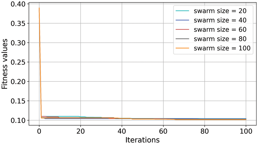
Figure 5: Various SSA-XGBoost models with different swarm sizes
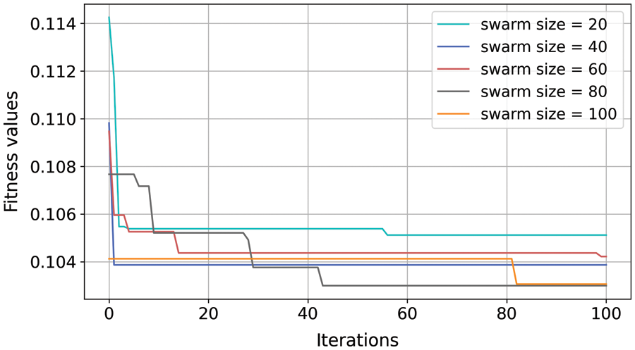
Figure 6: Various RS-XGBoost models with different swarm sizes
To more clearly identify the performance of the SSA-XGBoost and RS-XGBoost models, four evaluation metrics (i.e., the values of R2, RMSE, MAE, and VAF) were utilized to assess the accuracy and error of the hybrid XGBoost models. Note that the performance of a machine learning model should not only be considered on the training set but also the testing dataset plays an important role in assessing the prediction performance of the developed model. Based on this, the evaluation results of four evaluation metrics on the training and testing sets are summarized in Table 5. According to these four metrics, an excellent model has higher R2 and VAF, as well as lower RMSE and MAE. Consequently, based on the results in Table 5, it can be inferred that the SSA-XGBoost model with 40 swarms shows the best performance compared to other models. The R2 values of 0.977 and 0.849, the VAF values of 97.714 and 84.936, the RMSE values of 0.026 and 0.094, and the MAE values of 0.019 and 0.073 for the training and testing sets, respectively, confirm the feasibility of the SSA-XGBoost predictive model. In addition, the hyperparameters that were employed by the optimal model (i.e., the SSA-XGBoost model with 40 swarms) are the learning rate of 0.18 and the subsample of 0.41, respectively. Here, to visualize the actual position of the optimal solution in the domain space, the possible solutions in the domain space is displayed in Fig. 7 using a three-dimensional plot. In Fig. 7, the x-axis represents the learning rate, the y-axis represents the subsample, and the z-axis represents the fitness value. The red point indicates the best solution (i.e., the optimal hyperparameters), whose coordinates are (0.18, 0.41). The remaining points are the fitness values calculated on the intervals [0.01, 0.5] and [0.2, 0.8]. Intuitively, when the learning rate is too small, the value of the fitness is large, which means that the trained model suffers from underfitting.
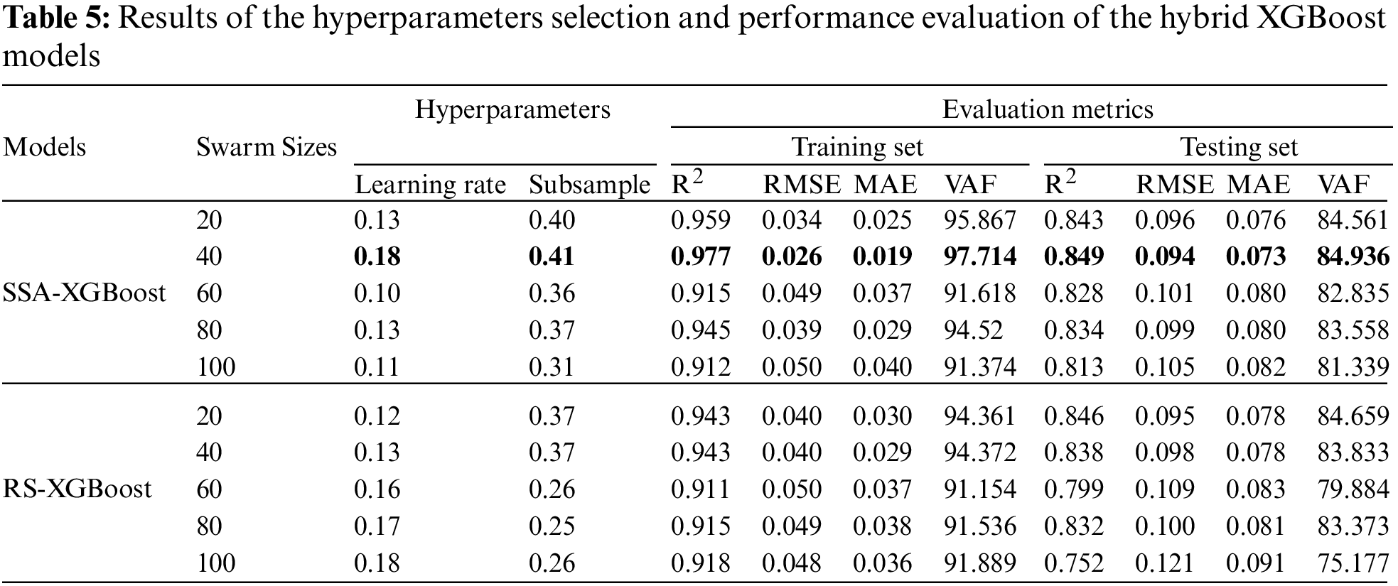
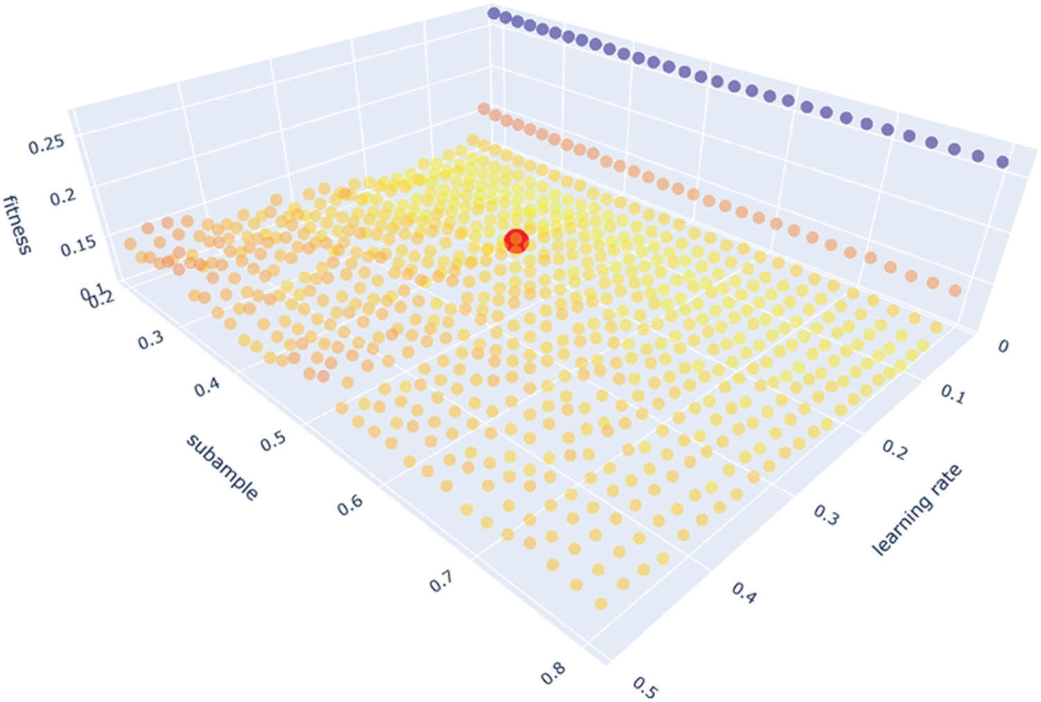
Figure 7: Optimal solution in the search space
To have a better understanding about the differences among these models (see Table 5), the evaluation metrics were categorized into two groups. The first category considers the 100 × R2 and VAF values of the models. Needless to say, in this category, a model with larger coordinate performs best. In the second category, the focus is on the MAE and RMSE values. Hence, a model with smaller coordinates indicates smaller errors (see Fig. 8).
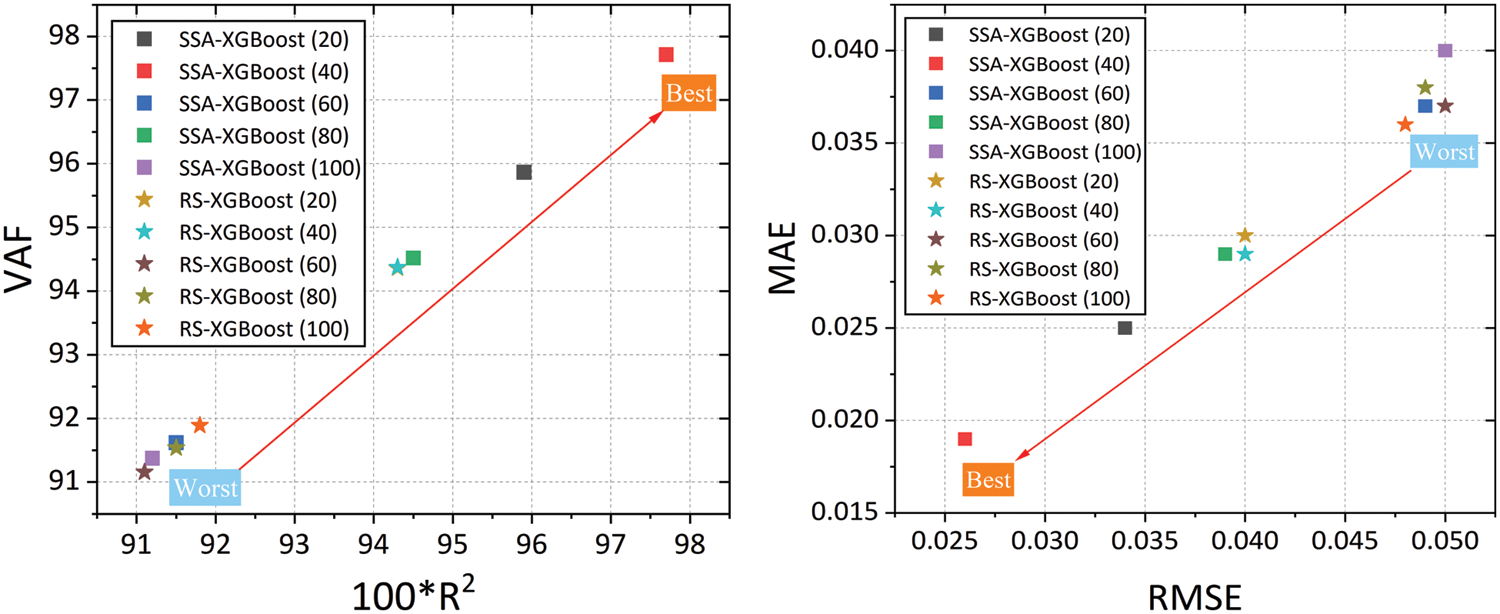
Figure 8: Performance of the proposed hybrid XGBoost models on the training set
Based on the above discussion, Fig. 8 (left side) suggests that SSA-XGBoost predictive model with 40 swarms outperforms other models in terms of VAF as well as R2 values. On the other hand, Fig. 8 (right side) also suggests that SSA-XGBoost predictive model with 40 swarms has the lowest error and works better in terms of MAE and RMSE values. In general, the SSA-XGBoost model outperforms the RS-XGBoost model for the training dataset. Similarly, Fig. 9 shows the prediction performances of the developed models for testing data. This figure also recommends that, in general, the SSA-XGBoost predictive model with 40 swarms outperforms the RS-XGBoost model for testing datasets. Overall, based on the prediction performances of the models for training and testing datasets, one can assert that the SSA-XGBoost model with 40 swarms is a feasible tool for assessing the shear strength of the soil.
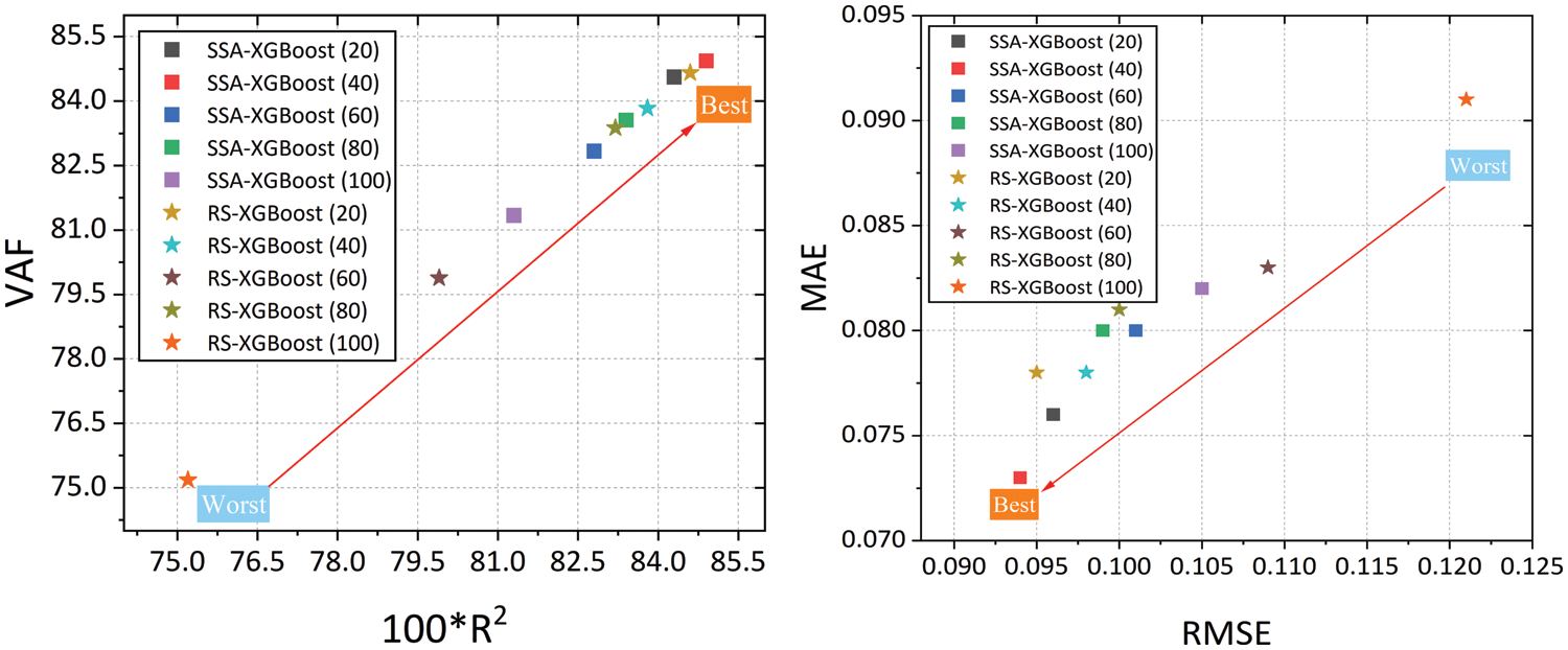
Figure 9: Performance of the proposed hybrid XGBoost models on the testing set
Finally, to visualize the difference between the predicted and true values, the measured and predicted shear strength by the SSA-XGBoost model with 40 swarms on both training and test sets are depicted, in Fig. 10. For the training set, it can be found that the proposed SSA-XGBoost model can predict the shear strength well enough because the data points are concentrated near the y = x line, while for the testing set, the distribution of data points around y = x line is not as good as the training set. This is because only 152 data samples were available in the present study. Hence, the presented database does not fully reflect the true scenario of the “real world”. Thus, the developed model does not perform very well on the testing (unknown) data set, which indicates that the model is overfitted. Although some measures such as tuning the subsample ratio were utilized to remedy the issue of overfitting, the number of available data is only 152 samples. This can lead to the relatively weak generalization ability of the XGBoost. Hence, to refine the prediction power of the model, an expanded and comprehensive database with additional samples should be employed. Alternatively, data augmentation techniques, such as generative adversarial network or variational autoencoder, can also be utilized to augment the data size.
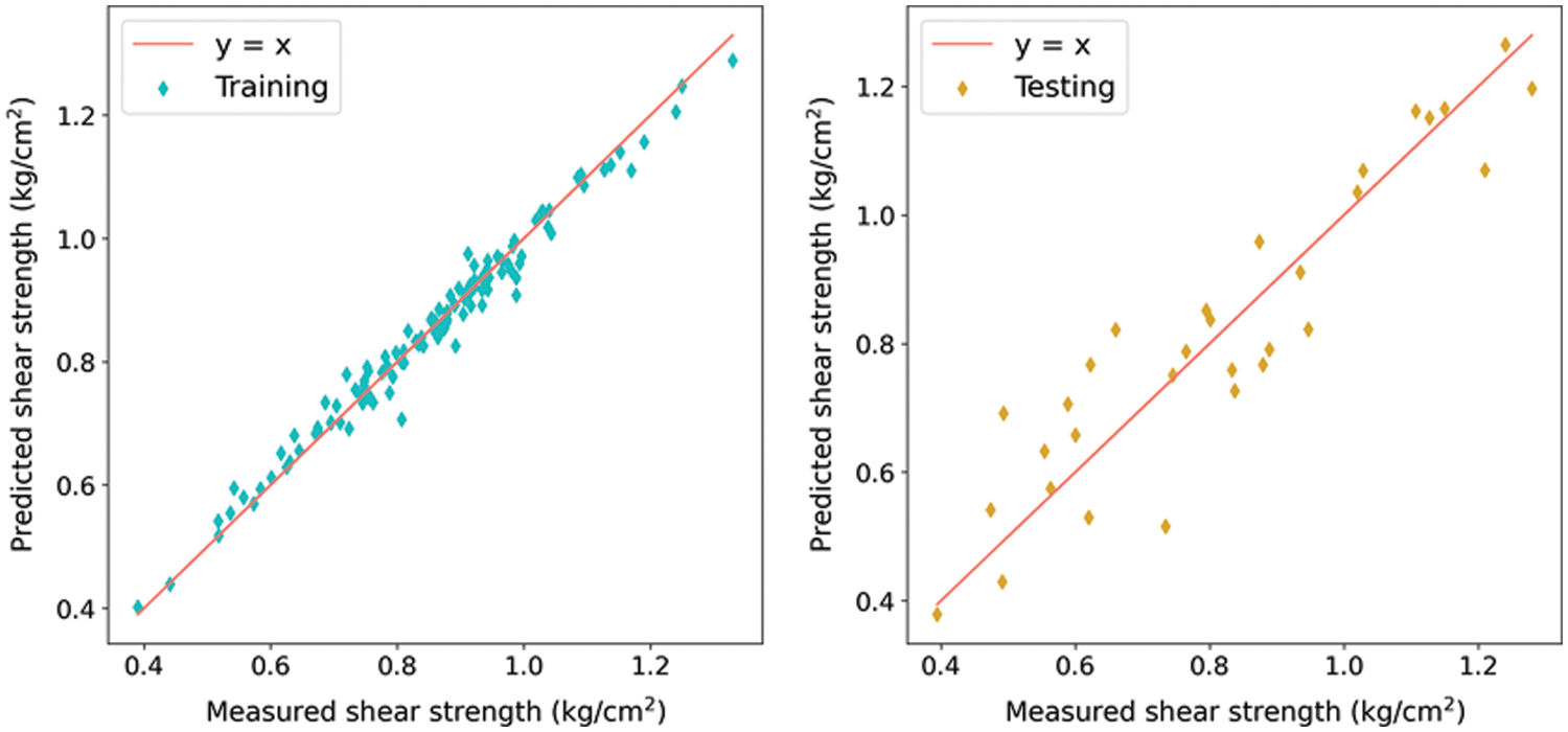
Figure 10: Predicted and measured shear strength of the SSA-XGBoost on the training (left one) and testing (right one) sets
4.2 Validation of Model Performance
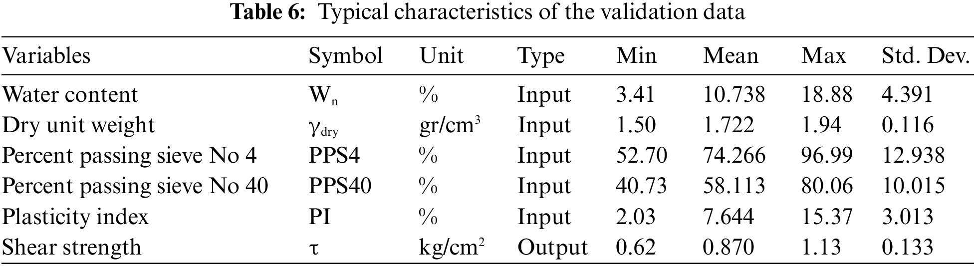
In this section, another 30 data samples (named validation data) were prepared from the same project to verify the generalization ability of the developed XGBoost model. Table 6 shows the statistical index of the validation data. A subtle discrepancy between the original data and validation data is the difference between the variable’s variance, for example, for variables Wn, PPS4, PPS40, and PI. Besides, the range of each variable was in good agreement with the range of the validation data. This can provide promising anticipation that the XGBoost model may show a favorable performance on the validation data.
Similar to the training and testing sets, the input variables in the validation phase include Wn, γdry, PPS4, PPS40, and PI. Then, the performance of the proposed XGBoost model on the validation data set was investigated and prediction results were checked against target values. According to the predictive result in Table 7, it can be seen that the values of RMSE and MAE (0.058 and 0.048, respectively) on the validation data set are smaller than the corresponding values (0.094 and 0.073, respectively) on the testing data set. On the other hand, the values of R2 and VAF (0.849% and 84.936%, respectively) on the testing set are higher compared to the validation data (0.805% and 83.379%, respectively). As we know, RMSE and MAE represent the predictive bias of a machine learning model, and R2 and VAF represent the predictive variance of a machine learning model. Thus, the above result reflects that the XGBoost model has a low predictive bias and a high predictive variance for the validation data set (in comparison with testing data set). This phenomenon implies that the proposed XGBoost model may have encountered overfitting on the validation set. Further, we provide a visualization of the predicted and measured soil strength from the validation data set, as shown in Fig. 11. Intuitively, most of the predicted and measured data samples are approximate, but some individual data samples show obvious differences which cause relatively high variance on the prediction performance of the XGBoost model for the validation data set. As mentioned previously, one feasible way to solve this problem (overfitting) is to supplement more data samples to the current data set.
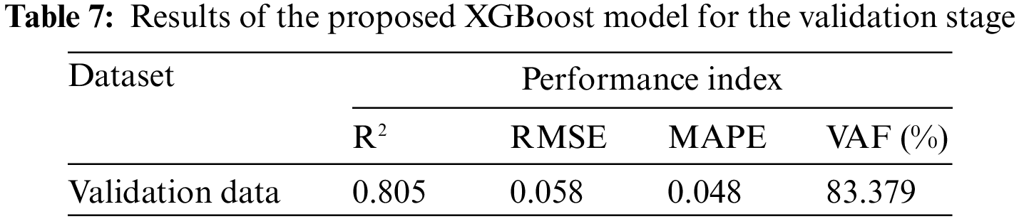
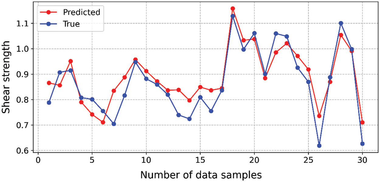
Figure 11: Predicted and measured shear strength values during the validation data
4.3 Sensitivity Analysis of Predictor Variables
A sensitivity analysis was conducted to identify the most influential input variables on the model output. As previously stated, five variables, i.e., moisture content, dry unit weight, percent passing sieve No 40, plasticity index, and percent passing sieve No 4, were used to construct the SSA-XGBoost predictive model of soil shear strength. The XGBoost model has the ability to filtrate the feature as the split node based on the gain of the structure score. In other words, more implementation of a feature for building a decision tree indicates its higher importance. The importance of a feature is the sum of its occurrences in all trees. Details on the theoretical background of the aforementioned sensitivity analysis are beyond the scope of this study and can be found elsewhere [59]. Nevertheless, on this basis, the importance of the input variables that were used to predict shear strength can be obtained (see Fig. 12). Overall, the related correlation of the Wn with shear strength is 0.376, the significant correlation of the γdry with shear strength is 0.164, the significant correlation of the PPS40 with shear strength is 0.160, the significant correlation of the PI with shear strength is 0.150, and the significant correlation of the PPS4 with shear strength is 0.149. Hence, for the considered dataset in this study, the most important input variable is the Wn, whereas the γdry, PPS40, PI, and PPS4 show a similar correlation with the shear strength. It is worth mentioning that for the multivariate problem of interest with unknown and complicated contact nature between dependent and independent variables, one input variable cannot heavily affect the model output (soil shear strength). In other words, the amount of PPS4 parameter (or Wn) alone is not a good index for assessing the soil shear strength as the latter is the function of several parameters. Especially for the problem of interest where the input parameters should be determined easily. Hence, it is not surprising that the mutual correlations between input parameters (e.g., γdry) and shear strength are not strong enough. However, when the multivariate problem is coupled with artificial intelligence using a prepared training set of data, a reliable predictive model can be developed. Nevertheless, the reliability of the developed models depends on the reliability of the feeding data (training data) and their ranges. Therefore, it is always recommended to practice the methods with different datasets.
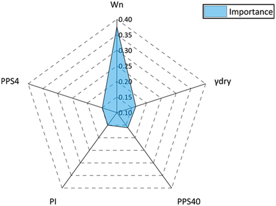
Figure 12: Significant correlation of the input variables with shear strength
5 Conclusion and Recommendation
This paper exploited the novel hybrid XGBoost models to predict shear strength. A total of 152 shear strength instances were used to develop the hybrid XGBoost models. The input parameters used for modeling included Wn, γdry, PPS40, PI, and PPS4, while the output was the shear strength. Then, two novel hybrid XGBoost models, i.e., the SSA-XGBoost model and the RS-XGBoost model, were constructed. The results confirmed that the SSA-XGBoost models outperform the RS-XGBoost models. This is attributed to the fact that in this study, the SSA was able to capture the hyperparameters of the XGBoost models more efficiently compared to the RS algorithm. The performance evaluation results of the SSA-XGBoost model showed the workability of the proposed model (the R2 values of 0.977 and 0.849, the VAF values of 97.714% and 84.936%, the RMSE values of 0.026 and 0.094, and the MAE values of 0.019 and 0.073 on the training and testing sets, respectively).
Future research in this area with different sets of data is highly recommended as the size of the dataset is of importance in model generalization. The broader range of input data can increase the prediction power of the future predictive models of soil shear strength. Although this study focused on the workability of the hybrid SSA-XGBoost predictive model, the implementation of other theory-guided machine learning techniques for the problem of interest and other soil mechanic problems is recommended.
Funding Statement: The authors received no specific funding for this study.
Availability of Data and Materials: Data will be made available from the corresponding author upon reasonable request.
Conflicts of Interest: The authors declare that they have no conflicts of interest to report regarding the present study.
References
1. Hatanaka, M., Uchida, A. (1996). Empirical correlation between penetration resistance and internal friction angle of sandy soils. Soils and Foundations, 36, 1–9. https://doi.org/10.3208/sandf.36.4_1 [Google Scholar] [CrossRef]
2. Shahin, M., Jaksa, M., Maier, H. (2002a). Artificial neural network–based settlement prediction formula for shallow foundations on granular soils. Australian Geomechanics, 37(4), 45–52. [Google Scholar]
3. Shahin, M. A., Maier, H. R., Jaksa, M. B. (2002b). Predicting settlement of shallow foundations using neural networks. Journal of Geotechnical and Geoenvironmental Engineering, 128(9), 785–793. https://doi.org/10.1061/(ASCE)1090-0241(2002)128:9(785) [Google Scholar] [CrossRef]
4. Sinha, S. K., Wang, M. C. (2008). Artificial neural network prediction models for soil compaction and permeability. Geotechnical and Geological Engineering, 26(1), 47–64. https://doi.org/10.1007/s10706-007-9146-3 [Google Scholar] [CrossRef]
5. Samui, P. (2008). Prediction of friction capacity of driven piles in clay using the support vector machine. Canadian Geotechnical Journal, 45, 288–295. https://doi.org/10.1139/T07-072 [Google Scholar] [CrossRef]
6. Shahin, M. A., Jaksa, M. B., Maier, H. R. (2008). State of the art of artificial neural networks in geotechnical engineering. Electronic Journal of Geotechnical Engineering, 8(1), 1–26. [Google Scholar]
7. Kuo, Y., Jaksa, M., Lyamin, A., Kaggwa, W. (2009). ANN-based model for predicting the bearing capacity of strip footing on multi-layered cohesive soil. Computers and Geotechnics, 36, 503–516. https://doi.org/10.1016/j.compgeo.2008.07.002 [Google Scholar] [CrossRef]
8. Gunaydın, O. (2009). Estimation of soil compaction parameters by using statistical analyses and artificial neural networks. Environmental Geology, 57, 203–215. https://doi.org/10.1007/s00254-008-1300-6 [Google Scholar] [CrossRef]
9. Park, H. I., Lee, S. R. (2011). Evaluation of the compression index of soils using an artificial neural network. Computers and Geotechnics, 38(4), 472–481. https://doi.org/10.1016/j.compgeo.2011.02.011 [Google Scholar] [CrossRef]
10. Johari, A., Javadi, A., Habibagahi, G. (2011). Modelling the mechanical behaviour of unsaturated soils using a genetic algorithm-based neural network. Computers and Geotechnics, 38, 2–13. https://doi.org/10.1016/j.compgeo.2010.08.011 [Google Scholar] [CrossRef]
11. Sezer, A. (2013). Simple models for the estimation of shearing resistance angle of uniform sands. Neural Computing and Applications, 22(1), 111–123. https://doi.org/10.1007/s00521-011-0668-5 [Google Scholar] [CrossRef]
12. Jahed Armaghani, D., Tonnizam Mohamad, E., Momeni, E., Sundaram Narayanasamy, M., Mohd Amin, M. F. (2015). An adaptive neuro-fuzzy inference system for predicting unconfined compressive strength and young’s modulus: A study on main range granite. Bulletin of Engineering Geology and the Environment, 74, 1301–1319. https://doi.org/10.1007/s10064-014-0687-4 [Google Scholar] [CrossRef]
13. Kiran, S., Lal, B., Tripathy, S. (2016). Shear strength prediction of soil based on probabilistic neural network. Indian Journal of Science and Technology, 9(41), 1–6. https://doi.org/10.17485/ijst/2016/v9i41/99188 [Google Scholar] [CrossRef]
14. Moavenian, M., Nazem, M., Carter, J., Randolph, M. (2016). Numerical analysis of penetrometers free-falling into soil with shear strength increasing linearly with depth. Computers and Geotechnics, 72, 57–66. https://doi.org/10.1016/j.compgeo.2015.11.002 [Google Scholar] [CrossRef]
15. Bathurst, R. J., Javankhoshdel, S. (2017). Influence of model type, bias and input parameter variability on reliability analysis for simple limit states in soil–structure interaction problems. Georisk: Assessment and Management of Risk for Engineered Systems and Geohazards, 11(1), 42–54. https://doi.org/10.1080/17499518.2016.1154160 [Google Scholar] [CrossRef]
16. Moayedi, H., Mosallanezhad, M., Rashid, A., Jusoh, W., Muazu, M. A. (2019). A systematic review and meta-analysis of artificial neural network application in geotechnical engineering: Theory and applications. Neural Computing and Applications, 32(2), 495–518. https://doi.org/10.1007/s00521-019-04109-9 [Google Scholar] [CrossRef]
17. Jahed Armaghani, D., Momeni, E., Asteris, P. G. (2020). Application of group method of data handling technique in assessing deformation of rock mass. The International Journal of Applied Metaheuristic Computing, 1, 1–18. [Google Scholar]
18. Nazir, R., Momeni, E., Marsono, K., Maizir, H. (2015). An artificial neural network approach for prediction of bearing capacity of spread foundations in sand. Jurnal Teknologi, 72, 9–14. https://doi.org/10.11113/jt.v72.4004 [Google Scholar] [CrossRef]
19. Momeni, E., Poormoosavian, M., Mahdiyar, A., Fakher, A. (2018). Evaluating random set technique for reliability analysis of deep urban excavation using monte carlo simulation. Computers and Geotechnics, 100, 203–215. https://doi.org/10.1016/j.compgeo.2018.03.012 [Google Scholar] [CrossRef]
20. Momeni, E., Yarivand, A., Dowlatshahi, M. B., Jahed Armaghani, D. (2020). An efficient optimal neural network based on gravitational search algorithm in predicting the deformation of geogrid-reinforced soil structures. Transportation Geotechnics, 26, 100446. https://doi.org/10.1016/j.trgeo.2020.100446 [Google Scholar] [CrossRef]
21. Armaghani, D. J., Harandizadeh, H., Momeni, E. (2021). Load carrying capacity assessment of thin-walled foundations: An ANFIS–PNN model optimized by genetic algorithm. Engineering with Computer. https://doi.org/10.1007/s00366-021-01380-0 [Google Scholar] [CrossRef]
22. Armaghani, D. J., Harandizadeh, H., Momeni, E., Maizir, H., Jian, Z. (2022). An optimized system of GMDH-ANFIS predictive model by ICA for estimating pile bearing capacity. Artificial Intelligence Review, 55, 2313–2350. https://doi.org/10.1007/s10462-021-10065-5 [Google Scholar] [CrossRef]
23. Asteris, P. G., Mamou, A., Hajihassani, M., Hasanipanah, M., Koopialipoor, M. et al. (2021). Soft computing based closed form equations correlating L and N-type schmidt hammer rebound numbers of rocks. Transportation Geotechnics, 29, 100588. https://doi.org/10.1016/j.trgeo.2021.100588 [Google Scholar] [CrossRef]
24. Lin, P., Chen, X., Jiang, M., Song, X., Xu, M. et al. (2022). Mapping shear strength and compressibility of soft soils with artificial neural networks. Engineering Geology, 300, 106585. https://doi.org/10.1016/j.enggeo.2022.106585 [Google Scholar] [CrossRef]
25. Momeni, E., Omidinasab, F., Dalvand, A., Goodarzimehr, V., Eskandari, A. (2022). Flexural strength of concrete beams made of recycled aggregates: An experimental and soft computing-based study. Sustainability, 14, 11769. https://doi.org/10.3390/su141811769 [Google Scholar] [CrossRef]
26. Khanlari, G. R., Heidari, M., Momeni, A. A., Abdilor, Y. (2012). Prediction of shear strength parameters of soils using artificial neural networks and multivariate regression methods. Engineering Geology, 131–132, 11–18. https://doi.org/10.1016/j.enggeo.2011.12.006 [Google Scholar] [CrossRef]
27. Kayadelen, C., Günaydin, O., Fener, M., Demir, A., Özvan, A. (2009). Modeling of the angle of shearing resistance of soils using soft computing systems. Expert Systems with Applications, 36, 11814–11826. https://doi.org/10.1016/j.eswa.2009.04.008 [Google Scholar] [CrossRef]
28. Khan, S. Z., Suman, S., Pavani, M., Das, S. K. (2016). Prediction of the residual strength of clay using functional networks. Geoscience Frontiers, 7, 67–74. https://doi.org/10.1016/j.gsf.2014.12.008 [Google Scholar] [CrossRef]
29. Das, S. K., Basudhar, P. K. (2008). Prediction of residual friction angle of clays using artificial neural network. Engineering Geology, 100, 142–145. https://doi.org/10.1016/j.enggeo.2008.03.001 [Google Scholar] [CrossRef]
30. Das, S. K., Samui, P., Khan, S. Z., Sivakugan, N. (2011). Machine learning techniques applied to prediction of residual strength of clay. Central European Journal of Geosciences, 3, 449–461. [Google Scholar]
31. Ding, W., Nguyen, M. D., Salih Mohammed, A., JahedArmaghani, D., Hasanipanah, M. et al. (2021). A new development of ANFIS-based henry gas solubility optimization technique for prediction of soil shear strength. Transportation Geotechnics, 29, 100579. https://doi.org/10.1016/j.trgeo.2021.100579 [Google Scholar] [CrossRef]
32. Armaghani, D. J., Mirzaei, F., Toghroli, A., Shariati, A. (2020). Indirect measure of shear strength parameters of fiber-reinforced sandy soil using laboratory tests and intelligent systems. Geomechanics and Engineering, 22, 397–414. [Google Scholar]
33. Kanungo, D. P., Sharma, S., Pain, A. (2014). Artificial neural network (ANN) and regression tree (CART) applications for the indirect estimation of unsaturated soil shear strength parameters. Frontiers in Earth Science, 8(3), 439–456. https://doi.org/10.1007/s11707-014-0416-0 [Google Scholar] [CrossRef]
34. Kiran, S., Lal, B. (2015). ANN based prediction of shear strength of soil from their index properties. International Journal of Earth Sciences and Engineering, 8, 2195–2202. [Google Scholar]
35. Tizpa, P., Jamshidi Chenari, R., Karimpour Fard, M., Lemos Machado, S. (2015). ANN prediction of some geotechnical properties of soil from their index parameters. Arabian Journal of Geosciences, 8, 2911–2920. https://doi.org/10.1007/s12517-014-1304-3 [Google Scholar] [CrossRef]
36. Pham, B. T., Son, L. H., Hoang, T. A., Nguyen, D. M., Bui, D. T. (2018). Prediction of shear strength of soft soil using machine learning methods. Catena, 166, 181–191. https://doi.org/10.1016/j.catena.2018.04.004 [Google Scholar] [CrossRef]
37. Kaya, A. (2009). Residual and fully softened strength evaluation of soils using artificial neural networks. Geotechnical and Geological Engineeing, 27, 281–288. https://doi.org/10.1007/s10706-008-9228-x [Google Scholar] [CrossRef]
38. Stark, T. D., Choi, H., McCone, S. (2005). Drained shear strength parameters for analysis of landslides. Journal of Geotechnical and Geoenvironmental Engineering, 131, 575–588.https://doi.org/10.1061/(ASCE)1090-0241(2005)131:5(575) [Google Scholar] [CrossRef]
39. Tien Bui, D., Hoang, N. D., Nhu, V. H. (2019). A swarm intelligence-based machine learning approach for predicting soil shear strength for road construction: A case study at trung luong national expressway project (Vietnam). Engineering with Computers, 35, 955–965. https://doi.org/10.1007/s00366-018-0643-1 [Google Scholar] [CrossRef]
40. Hashemi Jokar, M., Mirasi, S. (2018). Using adaptive neuro-fuzzy inference system for modeling unsaturated soils shear strength. Soft Computing, 22, 4493–4510. https://doi.org/10.1007/s00500-017-2778-1 [Google Scholar] [CrossRef]
41. Ly, H. B., Pham, B. T. (2020). Prediction of shear strength of soil using direct shear test and support vector machine model. The Open Construction and Building Technology Journal, 14, 268–277. https://doi.org/10.2174/1874836802014010268 [Google Scholar] [CrossRef]
42. Mousavi, M., Jiryaei Sharahi, M. (2021). Estimating the sand shear strength from its grain characteristics using an artificial neural network model and multiple regression analysis. AUT Journal of Civil Engineering, 5(3), 403–420. [Google Scholar]
43. Chao, Z., Fowmes, G., Dassanayake, S. M. (2021). Comparative study of hybrid artificial intelligence approaches for predicting peak shear strength along soil-geocomposite drainage layer interfaces. International Journal of Geosynthetics and Ground Engineering, 7, 1–19. https://doi.org/10.1007/s40891-021-00299-2 [Google Scholar] [CrossRef]
44. Jain, R., Jain, P. K., Bhadauria, S. S. (2010). Computational approach to predict soil shear strength. International Journal of Engineering Science and Technology, 2, 3874–3885. [Google Scholar]
45. Zhang, W., Wu, C., Zhong, H., Li, Y., Wang, L. (2021). Prediction of undrained shear strength using extreme gradient boosting and random forest based on Bayesian optimization. Geoscience Frontiers, 12, 469–477. https://doi.org/10.1016/j.gsf.2020.03.007 [Google Scholar] [CrossRef]
46. Dutta, R. K., Gnananandarao, T., Ladol, S. (2020). Soft computing based prediction of friction angle of clay. Archives of Materials Science and Engineering, 104, 58–65. https://doi.org/10.5604/18972764 [Google Scholar] [CrossRef]
47. Mohammadi, M., Fatemi Aghda, S. M., Talkhablou, M., Cheshomi, A. (2022). Prediction of the shear strength parameters from easily-available soil properties by means of multivariate regression and artificial neural network methods. Geomechanics and Geoengineering, 17, 442–454. https://doi.org/10.1080/17486025.2020.1778194 [Google Scholar] [CrossRef]
48. Besalatpour, A., Hajabbasi, M. A., Ayoubi, S., Afyuni, M., Jalalian, A. et al. (2012). Soil shear strength prediction using intelligent systems: Artificial neural networks and an adaptive neuro-fuzzy inference system. Soil Science and Plant Nutrition, 58(2), 149–160. https://doi.org/10.1080/00380768.2012.661078 [Google Scholar] [CrossRef]
49. Kakarla, P., Sharma, S., Kanungo, D. P., Pain, A., Anbalagan, R. (2013). Artificial neural network approach based indirect estimation of shear strength parameters of soil. Proceedings of Indian Geotechnical Conference, pp. 22–24. Roorkee, India. [Google Scholar]
50. Richard, J. A., Sa’don, N. M., Abdul Karim, A. R. (2021). Artificial neural network (ANN) model for shear strength of soil prediction. Defect and Diffusion Forum, 411, 157–168. https://doi.org/10.4028/www.scientific.net/DDF.411.157 [Google Scholar] [CrossRef]
51. Zhu, L., Liao, Q., Wang, Z., Chen, J., Chen, Z. et al. (2022). Prediction of soil shear strength parameters using combined data and different machine learning models. Applied Sciences, 12, 5100. https://doi.org/10.3390/app12105100 [Google Scholar] [CrossRef]
52. Al-zubaidy, D. S., Aljanabi, K. R., Zeyad Khaled, S. M. (2022). Prediction of shear strength parameters of gypseous soil using artificial neural networks. Journal of Engineering, 4(28), 39–50. https://doi.org/10.31026/j.eng.2022.04.03 [Google Scholar] [CrossRef]
53. ASTM, D3080 (1996). Annual book of ASTM standards, soil and rock construction, section 4. In: American society for testing and materials. Philadelphia, Pennsylvania: ASTM International. [Google Scholar]
54. Das, B. M., Sobhan, K. (2013). Principles of geotechnical engineering. Stamford, UCS: Cengage Learning. [Google Scholar]
55. Whitlow, R. (1990). Basic soil mechanics. Hoboken, New Jersey, USA: Prentice Hall. [Google Scholar]
56. Sharma, B., Bora, P. K. (2003). Plastic limit, liquid limit and undrained shear strength of soil—Reappraisal. Journal of Geotechnical and Geoenvironmental Engineering, 129, 774–777. https://doi.org/10.1061/(ASCE)1090-0241(2003)129:8(774) [Google Scholar] [CrossRef]
57. Chen, T., Guestrin, C. (2015). XGBoost: Reliable large-scale tree boosting system tianqi. Proceedings of the 22nd SIGKDD Conference on Knowledge Discovery and Data Mining, pp. 13–17. San Francisco, CA, USA. [Google Scholar]
58. Chen, T., Guestrin, C. (2016). XGBoost: A scalable tree boosting system. ACM SIGKDD International Conference on Knowledge Discovery and Data Mining, pp. 785–794. San Francisco. [Google Scholar]
59. Liu, Z., Armaghani, D. J., Fakharian, P., Li, D., Ulrikh, D. V. et al. (2022). Rock strength estimation using several tree-based ML techniques. Computer Modeling in Engineering & Sciences, 133(3), 799–824. https://doi.org/10.32604/cmes.2022.021165 [Google Scholar] [CrossRef]
60. Mirjalili, S., Gandomi, A. H., Mirjalili, S. Z., Faris, H., Saremi, S. et al. (2017). Salp swarm algorithm: A bio-inspired optimizer for engineering design problems. Advances in Engineering Software, 114, 163–191. https://doi.org/10.1016/j.advengsoft.2017.07.002 [Google Scholar] [CrossRef]
61. Abualigah, L., Shehab, M., Alshinwan, M., Alabool, H. (2020). Salp swarm algorithm: A comprehensive survey. Neural Computing & Applications, 32, 11195–11215. https://doi.org/10.1007/s00521-019-04629-4 [Google Scholar] [CrossRef]
62. Zabinsky, Z. B. (2009). Random search algorithms. Hoboken, New Jersey, United States: Wiley Online Library. [Google Scholar]
63. Xu, H., Zhou, J., Asteris, P. G., Armaghani, D. J., Tahir, M. M. (2019). Supervised machine learning techniques to the prediction of tunnel boring machine penetration rate. Applied Sciences, 9, 1–19. https://doi.org/10.3390/app9183715 [Google Scholar] [CrossRef]
64. Zhou, J., Dai, Y., Khandelwal, M., Monjezi, M., Yu, Z. et al. (2021). Performance of hybrid SCA-RF and HHO-RF models for predicting backbreak in open-pit mine blasting operations. Natural Resources Research, 30, 4753–4771. https://doi.org/10.1007/s11053-021-09929-y [Google Scholar] [CrossRef]
65. Zhou, J., Zhu, S., Qiu, Y., Armaghani, D. J., Zhou, A. et al. (2022). Predicting tunnel squeezing using support vector machine optimized by whale optimization algorithm. Acta Geotechnica, 7. https://doi.org/10.1007/s11440-022-01450-7 [Google Scholar] [CrossRef]
66. Zheng, H., Yuan, J., Chen, L. (2017). Short-term load forecasting using EMD-LSTM neural networks with a xgboost algorithm for feature importance evaluation. Energies, 10(8), 1168. https://doi.org/10.3390/en10081168 [Google Scholar] [CrossRef]
67. He, B., Lai, S. H., Mohammed, A. S., Sabri, M. M. S., Ulrikh, D. V. (2022). Estimation of blast-induced peak particle velocity through the improved weighted random forest technique. Applied Sciences, 12, 5019. https://doi.org/10.3390/app12105019 [Google Scholar] [CrossRef]
Cite This Article
 Copyright © 2023 The Author(s). Published by Tech Science Press.
This work is licensed under a Creative Commons Attribution 4.0 International License , which permits unrestricted use, distribution, and reproduction in any medium, provided the original work is properly cited.
 Downloads
 Citation Tools